Article

Carbon in Mature Native Forests in Australia: The Role of Direct Weighing in the Derivation of Allometric Equations

1
NSW Department of Primary Industries—Forest Science Unit, Parramatta 2124, Australia
2
VicForests, Melbourne 3000, Australia
3
Forestry Corporation of NSW, Wauchope 2446, Australia
4
Latitude Forest Services, Malua Bay 2536, Australia
5
NSW Office of Environment and Heritage, Hurstville 2220, Australia
*
Author to whom correspondence should be addressed.
Forests 2018, 9(2), 60; https://doi.org/10.3390/f9020060
Submission received: 30 November 2017 / Revised: 18 January 2018 / Accepted: 24 January 2018 / Published: 26 January 2018
(This article belongs to the Section Forest Ecology and Management)

Abstract

:
Accurate estimates of forest biomass are essential to understand the contribution of forests to climate change mitigation efforts. In this manuscript, we report on biomass determinations for 586 directly weighed trees located in three important native forest areas in Australia. The sites were paired according to management strategy; i.e., managed for periodic cycles of harvest or conservation only. The key aim of the work was to test whether non-site specific available biomass relationships are reliable, especially in the estimation of the biomass of trees with a large diameter at breast height (DBH). The above-ground carbon (AGC) estimates for largely undisturbed forests ranged from approximately 200–400 t C ha−1. Existing allometric equations were generally poor at estimating biomass for mature trees, especially those of large DBH. Direct weighing of biomass ensured a degree of certainty in the results that cannot be associated with previous studies that relied on sub-sampling, or with studies that relied on existing allometric equations. Thus, caution should be exercised when interpreting the results of previous studies that did not rely on direct weighing of the biomass in the context of decisions around optimum forest management regimens, and the contribution of mature forest stands to the global carbon balance.

1. Introduction

Forests are an important component of the global carbon cycle, primarily via the sequestration and storage of carbon, contributing to climate change mitigation [1]. Reporting of forest carbon stocks is an administrative requirement for participants in the United Nations Framework Convention on Climate Change [2], and signatory countries of the Kyoto Protocol are required to account for forest carbon stock changes [3]. Carbon is also one of the criteria listed under the “Montreal Process for the Conservation and Sustainable Management of Temperate and Boreal Forests”, as Criterion 5: “Maintenance of forest contribution to global carbon cycles” [4]. The sustainable management of native forests for continued wood production and their management for conservation purposes alone have been put forward as desirable pathways in the context of climate policy [5,6,7,8,9,10,11]. In both cases, however, it is critical to have accurate estimates of forest carbon for the range of diameter classes represented in the forest.
The biomass estimates which are used to derive above-ground carbon (AGC) are usually determined indirectly; either by the use of biomass expansion factors applied to traditional forest inventory measurements; or alternatively by applying existing biomass or allometric equations to parameters easily measured in the field such as diameter at breast height (DBH) and tree height [2]. The use of remote-sensing techniques such as LiDAR has more recently been promoted, as they potentially enable increasingly detailed assessments of spatial variation of forest biomass over large spatial scales—their accuracy, however, depends on calibration with field-derived data [12].
Allometric equations that are used for biomass determinations in native forests are often limited in their range, and typically do not include sufficient data for old and large trees [13,14]. Large trees are difficult to access, logistically challenging, and costly to weigh in large enough numbers in the field. However, it is very important that the database for biomass regression equations contains trees with large DBH as these tend to account for a large proportion of the aboveground biomass (AGB) in mature forests [13]. Uncertainty associated with biomass estimation of large trees is often ignored in practice [14]. In the tropics, for example, allometric equation selection has been shown to be the main source of error in field-based biomass estimates, primarily due to the limited sample size of trees used to generate allometric equations [15,16]. Extrapolating the intended range of the model potentially introduces significant bias and additional uncertainty to biomass estimates [17]. Similar issues with the application of existing allometric equations have been reported for biomass estimation in mature softwood trees [18]. Another key factor often neglected or dealt with in a limited fashion in the formulation of biomass equations for native forests is the impact of decay. Decay is not uniform and typically increases as the trees grow older, with the formation of hollows and eventual loss of limbs resulting in the loss of biomass. The use of allometric equations that are not developed based on weighed biomass data to predict biomass (and carbon stocks) in mature forest stands may result in unreliable estimates. In this manuscript, we report on biomass determinations for 586 directly weighed trees located in three important native forest areas in the States of New South Wales (NSW) and Victoria (VIC), in South-east (SE) Australia. Direct weighing of a number of mature trees with large DBH is often considered impractical and costly; however, the weighing system used in this study allowed biomass determination for a large number of such trees in each of the study sites. The forests selected are significant from a carbon sequestration perspective; it has been suggested that some of the most carbon-rich forests in the world are in SE Australia [19]. The sites were paired according to management strategy; i.e., managed for production purposes (hereafter referred to as “production sites”) or conservation only (hereafter referred to as “conservation sites”). The conservation sites were selected on the basis of their age and lack of significant known human intervention. The data was gathered as part of a larger project which assessed the greenhouse balance of native forest management for selected forest types in Australia, taking into account carbon dynamics in forests and in harvested wood products [20].
The key aims of the work were to introduce new allometric equations for the dominant species in each study site and to test whether non-site specific available biomass relationships are reliable, especially in the estimation of the biomass of native forest trees with large DBH (defined in this study as trees with DBH greater than 60 cm).

2. Materials and Methods

2.1. Site Description

The study sites included two native forest types in NSW and one in VIC in SE Australia; in Table 1, key descriptive information for each site is summarised. More information on the study sites is included in Appendix A and also in [20]. The dominant species were blackbutt (Eucalyptus pilularis Sm.), silvertop ash (Eucalyptus sieberi L.A.S. Johnson), and mountain ash (Eucalyptus regnans F. Muell.), for the NSW mid-north coast, NSW south coast, and VIC central highlands, respectively (Table 1). As described in [20], shrub cover for silvertop ash stands was mostly made up of saw banksia (Banksia serrata L.f.) and wattle (Acacia spp.). Shrub cover for the blackbutt production site was mostly made up of casuarina trees (Casuarina spp.), wattle, and rainforest species, whereas for the blackbutt conservation site, it was mostly made up of saw banksia and corkwood (Cryptocarya spp.). Shrub cover for the mountain ash stands was mostly made up of Correa spp and tree ferns.
The conservation mountain ash site was not available for harvest and therefore the biomass was estimated indirectly (more details in Section 2.4). The sites were selected in consultation with local foresters to ensure the production sites were representative of forests ready for timber harvest, and conservation sites were representative of forest sites largely unmanaged and with a large cohort of large trees, typically much older than those in the production sites. All sites presented evidence of past bushfires [20]. The only site that was subjected to a thinning event in the past was the mountain ash production site, which was thinned for pulpwood at age 29, with approximately a 50% reduction in stems.

2.2. Tree Measurements

At each site, a plot of approximately 0.5 ha was established. All the standing trees within the plot with a DBH greater than 10 cm were identified to species (excluding dead standing trees), numbered, and their DBH and height measured [20].

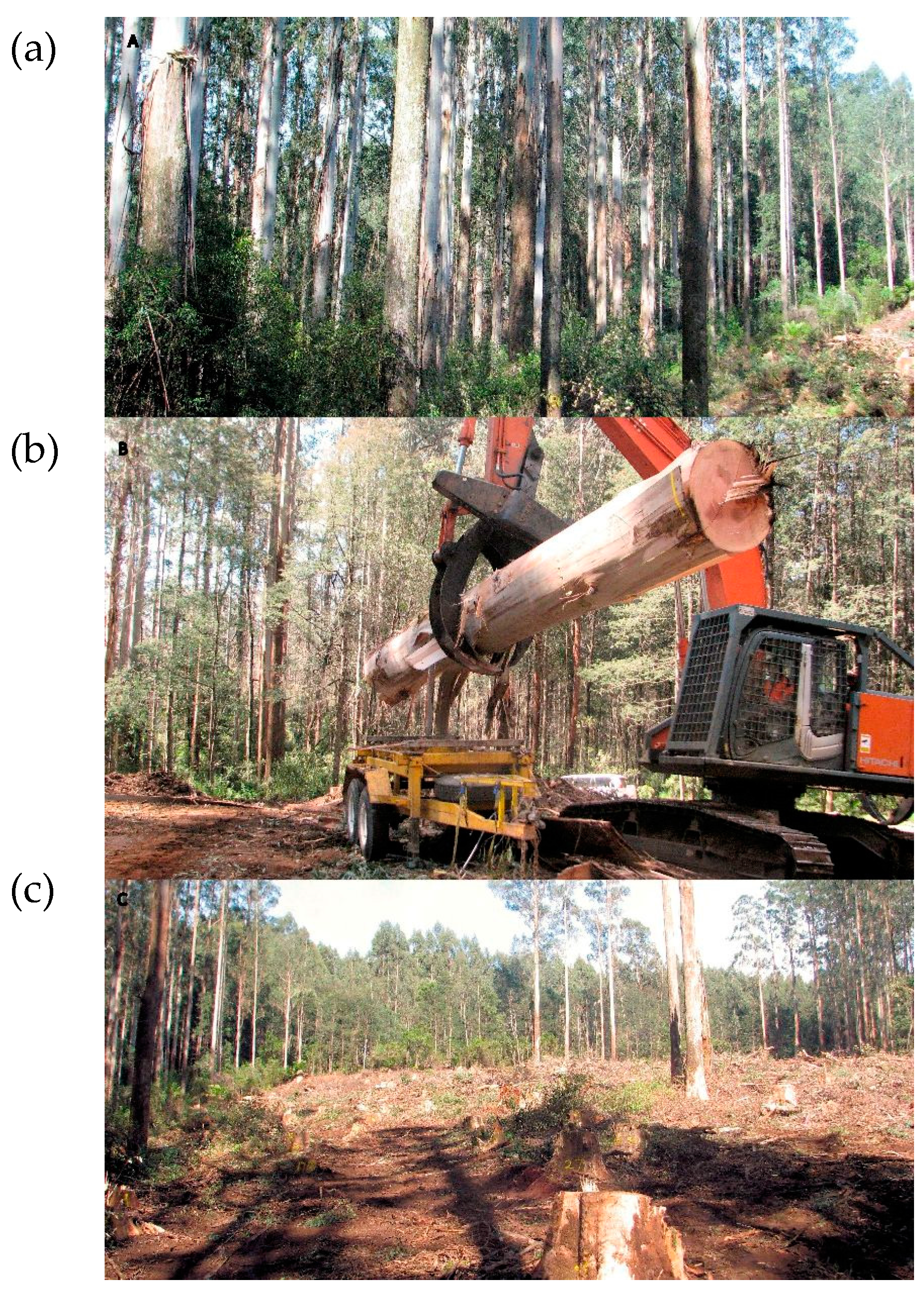
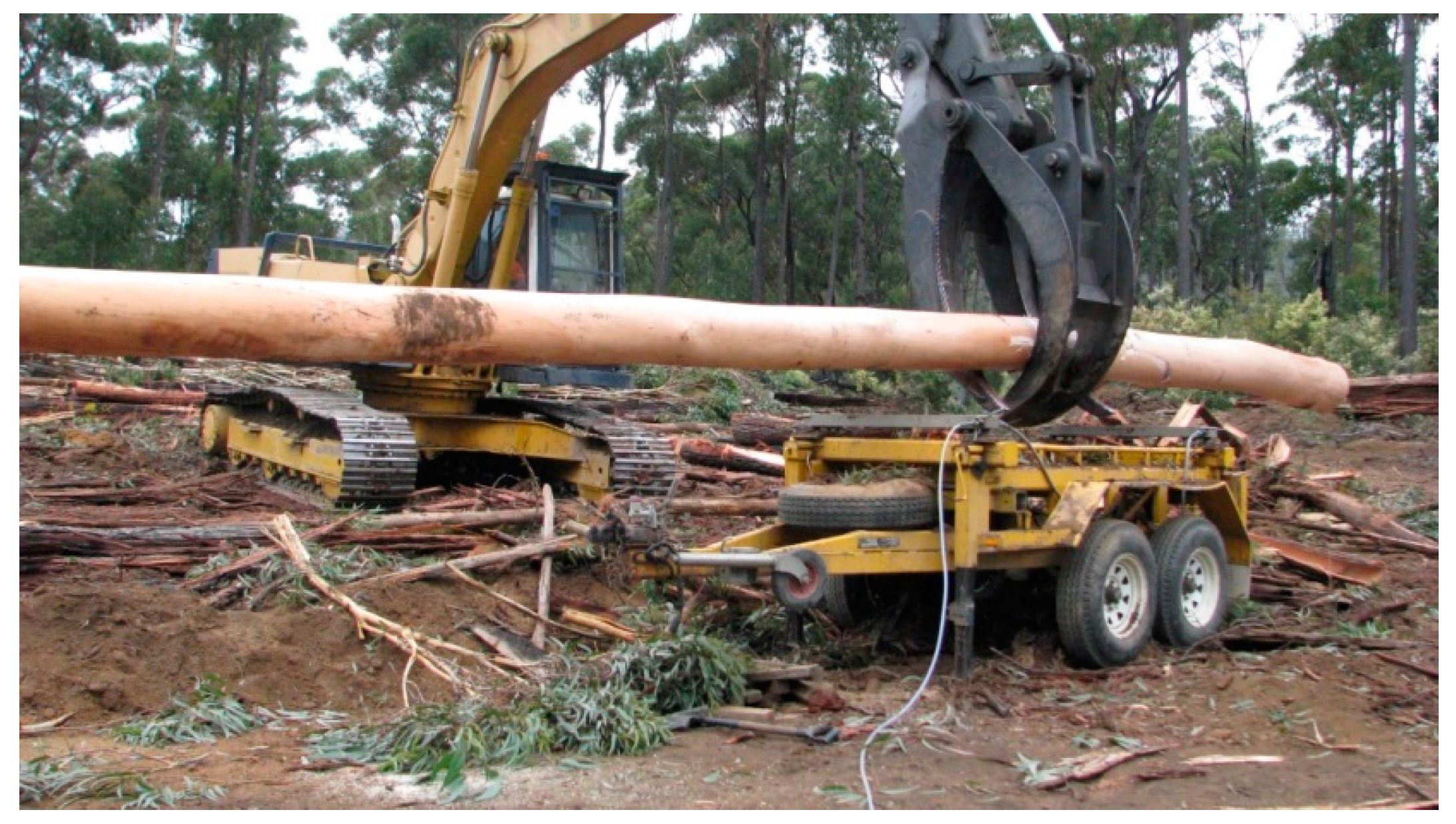
2.3. Weight Determinations in the Field

The weight determinations described here are more fully described in [20]. Tree components were weighed using a purpose built biomass-weighing trailer (Figure 1), fitted with weigh bars equipped with two load cells with a combined capacity of 5 tonnes. Weight increments of 1.0 kg are displayed on a digital display. Further details on the methodology used for weighing tree biomass using the biomass weighing trailer have been described previously [21].
For trees that yielded logs of a commercial quality, where possible, the weight of each commercial log was recorded with the bark on, and then with the bark removed. A visual estimation was made of any bark loss. For practical reasons, the crown component was only weighed with the bark intact. The weight of leaves was included in the weight of the crown. The starting point for the “crown” of production trees was defined as the point where the stem was too small to be of commercial value. The minimum diameter for cutting at the crown depended on whether a pulp market was available; with an 8 cm minimum diameter cut-off for those areas with a pulp market. The biomass in stumps was estimated based on the calculation of their volume, assuming for practical reasons that they approached the form of a cylinder. The stump height varied depending on factors such as species and tree size, ranging between 5 cm and 150 cm. The measured volume of the stump and the density of the base disc extracted were used to determine stump biomass.

2.4. Biomass Estimation

The biomass (oven-dry weight) of the stem, bark, and crown components of each tree was calculated, where possible, based on the average moisture content determined for each of those components (more details in Appendix B). If the stem bark weight for a given tree was not available, a bark:stem weight ratio was derived based on the same species and DBH class, from which a bark weight was derived. The weight of the leaves was included in the crown component of the trees, as it was impractical to weigh the leaves separately in the field. The following equation was applied to derive the biomass (oven-dry weight) for the calculated stump volume (Equation (1)):
StODW   ( kg )   = Basic   Density   ( kg / m 3 ) × Green   Volume   ( m 3 ) ,
The total AGB for each tree was the sum of the weight of each component. Tree biomass estimates were converted into carbon assuming a default carbon concentration of 50% [3], without considering potential differences in the carbon concentration of certain biomass fractions (e.g., leaves), which were not weighed separately in this study.
As it was not possible to directly weigh biomass at the mountain ash conservation site, the biomass was estimated based on allometric equations developed for the mountain ash production site, including thirteen large trees (DBH 101–131 cm) from a nearby stand that were directly weighed.

2.5. Selected Allometric Equations for Biomass Estimates

A number of allometric equations were identified in the literature as potentially applicable to our study sites and used to estimate biomass as a way of comparison with weighed data from the study sites. (Table 2). Please note that the equation developed by Keith et al. [22] listed in Table 2 is a generic equation for native sclerophyll forests. A more detailed description on how those relationships were derived is included in Appendix C.

2.6. Statistical Methods

Exploratory data analysis (EDA) is an analytical approach that focuses on identifying general patterns in the data, and identifying outliers and features that might not have been anticipated [30]. EDA using summary statistics, correlations, and plots was carried out to gain an understanding of the relationships between variables such as DBH, height, and biomass.
As the biomass data was highly skewed, log transformation (ln) was used to normalise the data. Regression models were fitted to the data and the species and type effects were tested to determine whether there was a significant effect of these variables on the allometric equations. Likelihood ratio tests and t statistics were used to identify the significant terms in the model. Analyses of the DBH:biomass plots identified a number of data points as high leverage points. These data points were checked for data entry errors prior to inclusion in the analysis, as inclusion of these points could result in a biased regression estimate. Therefore, robust regression was used, as a compromise between excluding these points entirely from the analysis and including all the data points and treating all of them equally as in ordinary least square (OLS) regression.
Robust regression is a form of weighted and reweighted least squares regression and it is fitted using the ‘rlm’ command in MASS package in R for deriving allometric equations. M-estimation with Huber weighting was used. The weighted regression equation is solved using Iteratively Reweighted Least Squares. The process continues until it converges. In Huber weighting, observations with small residuals are given a weight of 1—the larger the residual, the smaller the weight. The weight function for error is defined as (Equation (2)):
w ( e ) = { 1 for   | e | k k | e | for   | e | > k } ,
where e is the residual error and k = 1.345σ (where σ is the standard deviation of the errors).
The model was validated by inspecting the residual plots to check for homogeneity, independence, and normality. The accuracy of different allometric equations was assessed using the difference of the predicted value and the measured biomass value and plotting this difference against DBH.
Jolliffe and Stephenson [31] propose that the accuracy of models can be compared using the Mean Absolute Error (MAE). It is defined as (Equations (3) and (4)):
MAE = 1 n abs ( y obs   y pred ) n ,
and bias
bias ( y i ) = 1 n ( y pred y obs ) n ,
where n is the number of trees, yobs is the observed total dry weight biomass value, and ypred is the predicted value. MAE and bias were calculated in relative terms (MAE% and Bias %), i.e., the MAE and bias values for the biomass divided by the observed mean value and multiplied by 100. Linear regression was fitted to the predicted values from the different models and actual values; the slope values were tested to see if they were significantly different from 1, where a slope value of 1 would indicate a perfect fit. Nash-Sutcliffe efficiency (NSE) was also calculated instead of R2 for all models. NSE is a normalized statistic that determines the relative magnitude of the residual variance compared to the measured data variance [32]. Nash-Sutcliffe efficiencies range from −Inf to 1. Essentially, the closer to 1 the value is, the more accurate the model is. NSE = 1 corresponds to a perfect match of the modelled and observed data, NSE = 0 indicates that the model predictions are as accurate as the mean of the observed data, and −Inf < NSE < 0 indicates that the observed mean is a better predictor than the model. Similarly, high MAE% indicates less accuracy and higher absolute bias% indicates more bias in estimation. All analyses were carried out using R [33], MASS [34], and hydroGOF [35], and plotting was carried out using ggplot2 [36] and lattice [37].

3. Results

3.1. Forest Structure

The stand characteristics for the study sites are included in Table 3 [20]. The data reflects the differences in maturity between the paired sites, with higher mean DBH and basal area and lower total stems per hectare and stand density for the conservation sites (Table 3) [20]. Tree height did not change significantly between production and conservation sites (Table 3).

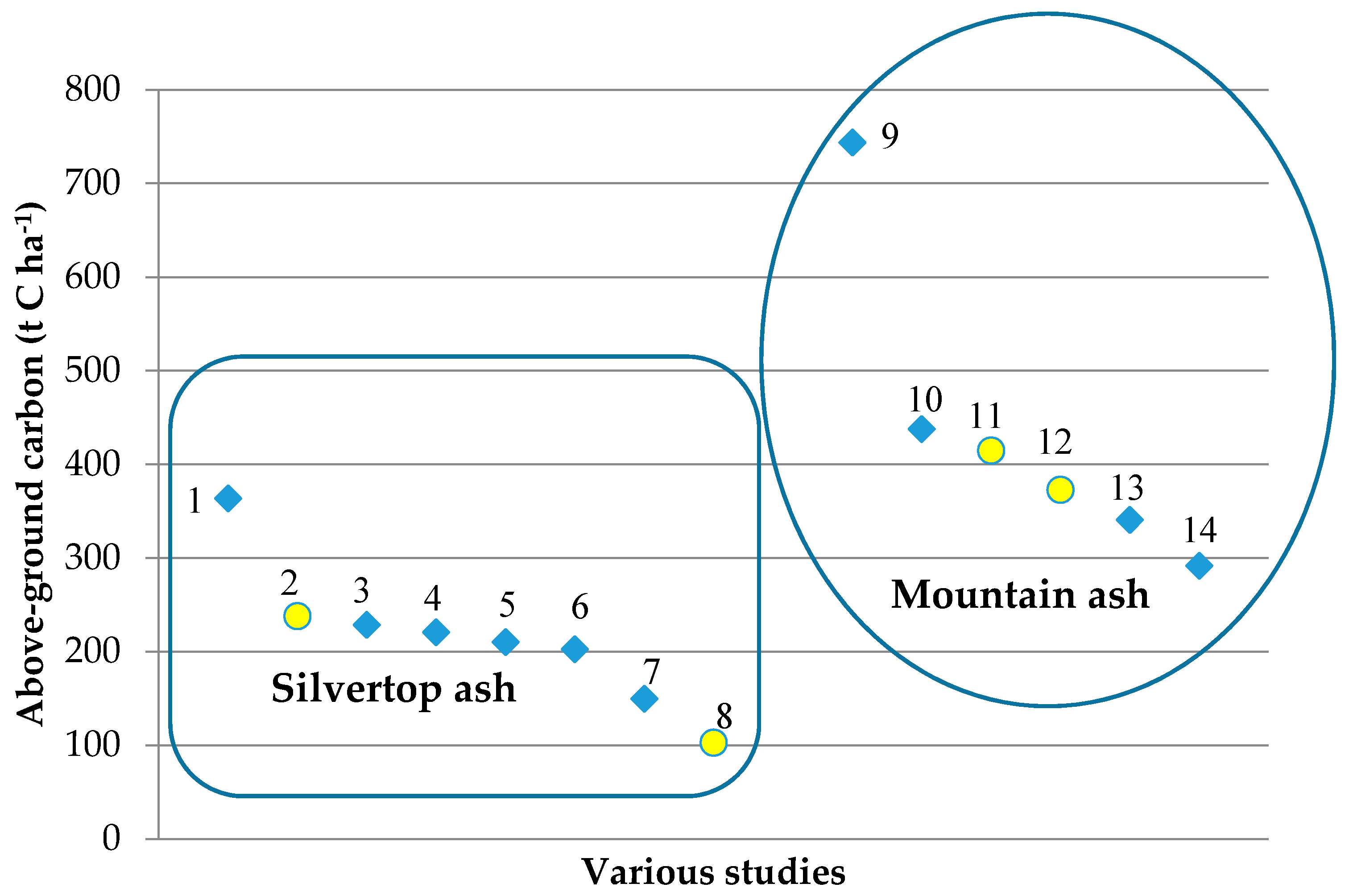
3.2. Standing Above-Ground Biomass (AGB)—Tree Component and Total Biomass

Data on the moisture content and density of individual tree components and also on the distribution of biomass by DBH class are included in Appendix C. The AGB in the conservation sites was much larger than that of the equivalent production sites, with the highly productive mountain ash sites having the highest AGB (Table 4). While the estimated AGB for the mountain ash conservation site was higher than the AGB for the paired production site, the relative difference was much less than for the NSW production and conservation sites (Table 4). The dominant species accounted for the majority of the AGB in the study sites (Table 4). A high proportion of the AGB in silvertop ash trees was in the bark (Table 4). Stewart et al. [29] reported even higher values (20%) for the relative contribution of the stem bark to the AGB in silvertop ash trees in VIC. As logs in native hardwood harvest operations are debarked in the forest, the differences in bark proportion between species can have a marked impact on the total amount of harvest residue left in the forest—this is exemplified by the differences between the bark contributions relative to the total AGB for mountain ash and silvertop ash (Table 4), [20]. From generic observations in the study sites, mountain ash trees in the production site were largely devoid of decay, whereas the mature trees in the NSW conservation sites had frequent evidence of decay, which was deemed more prevalent than in the equivalent production sites.
The AGB values in Table 4 were converted to AGC and compared with estimates from other relevant studies (Figure 2). As the literature on AGC for blackbutt-dominated forests is sparse, the comparisons were restricted to the silvertop ash and mountain ash stands (Figure 2). The method employed to derive AGB from the cited studies varied, but generally involved the use of previously developed allometric equations. For silvertop ash forests largely undisturbed by human activity, there was generally good agreement between AGC reported here and from previous studies with matching geographical coverage (Figure 2). The differences in AGC were greater for mountain ash stands (Figure 2).

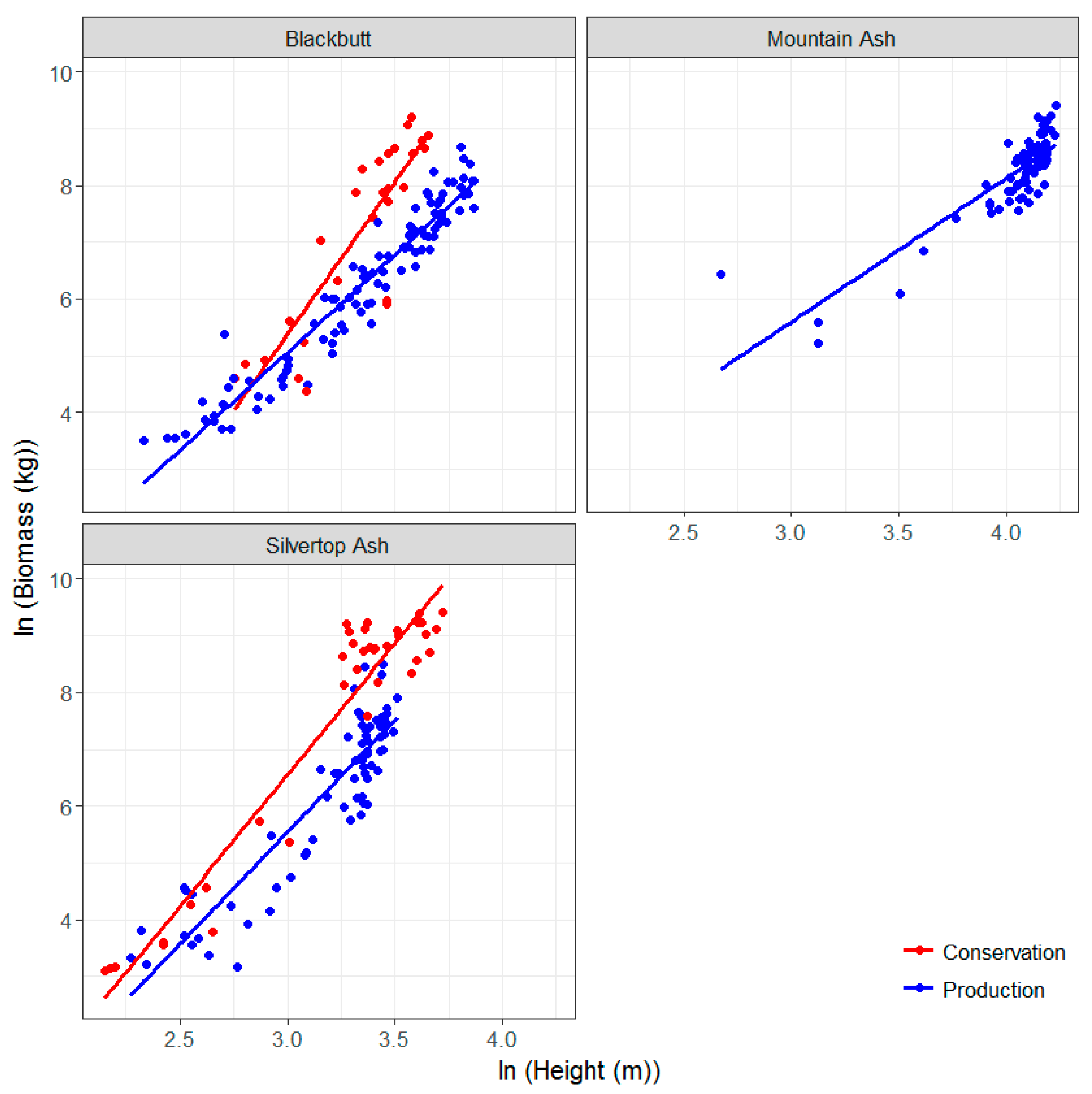
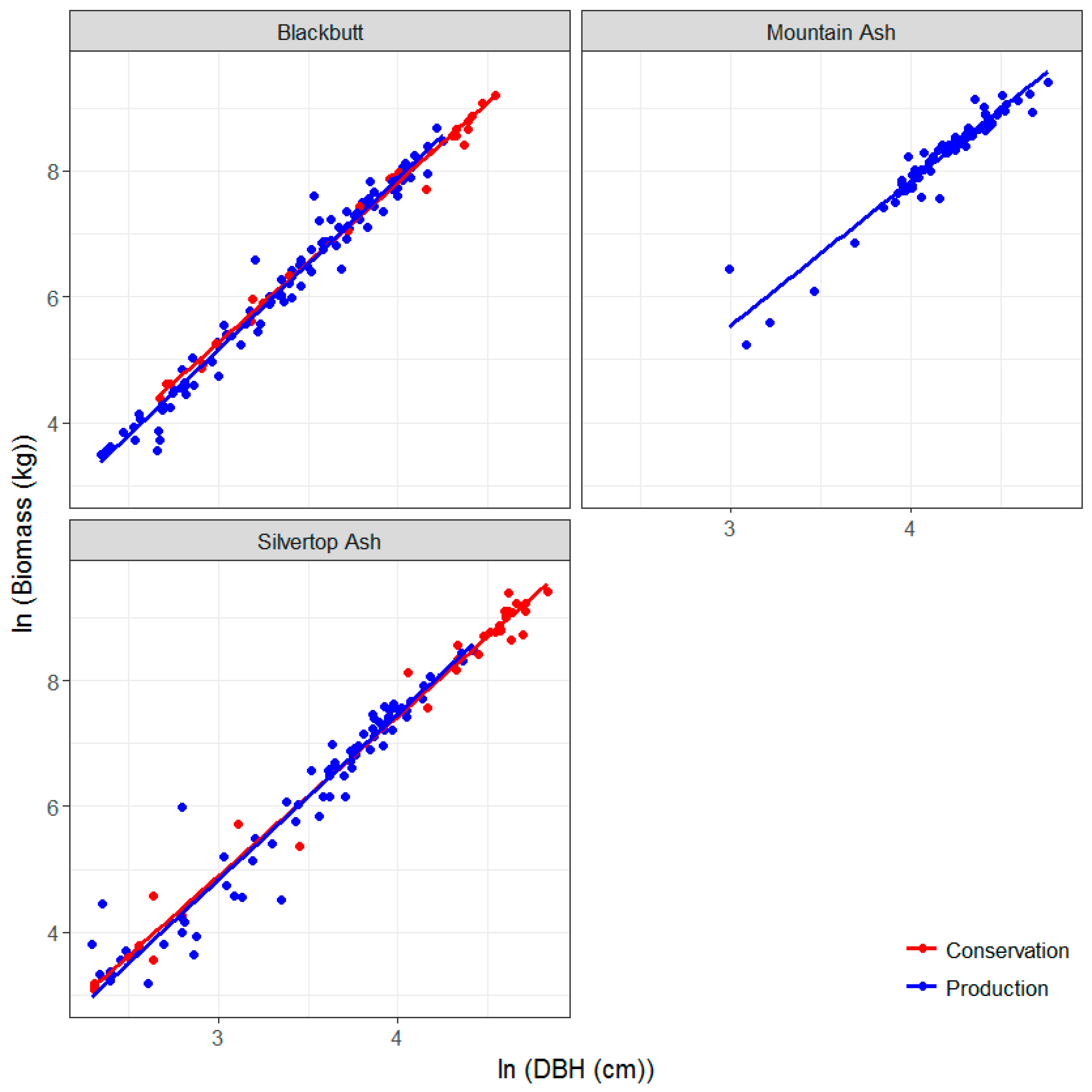
3.3. Allometric Equations for Key Species in the Study Sites: Development and Comparison with Existing Equations

One of the key applications of directly weighed tree biomass data is in the development of allometric equations. The equations based on DBH only were strong, and as expected, more robust than the equations based on height alone (Figure 3 and Figure 4 and Table 5). Adding height to the equations based on DBH alone improved their performance for all species (Table 5 and Figure 5, Figure 6 and Figure 7). As the main focus of this paper was on total tree biomass estimates and impacts of carbon estimation at the stand level, the development of allometric equations by individual biomass fractions (e.g., stem, leaves, bark) will be considered in a future manuscript, where the allometry of the key species in this study will be explored further. Stand structure (i.e., whether predominantly regrowth as was the case for production sites or old-growth stands as was the case for conservation sites) did not have a significant effect on the equations based on DBH for the same species (Figure 4). However, the linear equations based on height only were different when the paired sites for the same dominant species were compared (Figure 3). Additionally, for all relationships, the species effects appeared significant (Figure 3 and Figure 4). A multiple linear regression model was fitted to ln biomass as a response variable and ln DBH, species, and site as the predictor variables. For ln biomass and ln DBH equations, site was not significant (p = 0.38), whereas the species effect and ln DBH effect were highly significant (p < 0.0001). Thus, biomass data for the paired sites was combined in the formulation of allometric equations based on DBH only and also combined DBH and height, with strong correlations for all new proposed relationships (Table 5), providing a solid basis for comparisons with existing equations (Section 3.3). For a model with ln height, species, and site variables as predictors, all the variables were highly significant (p < 0.0001).

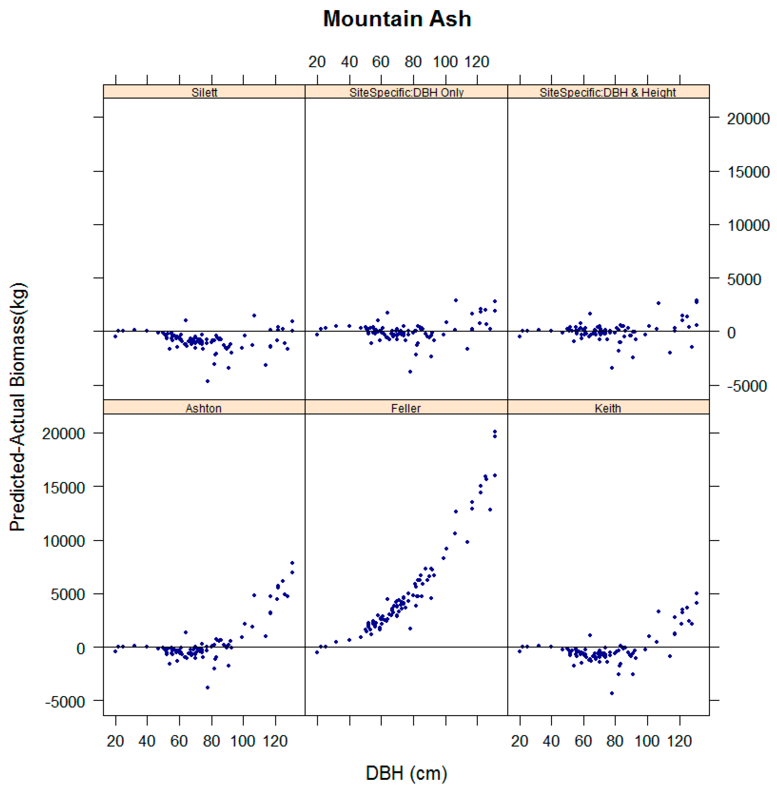
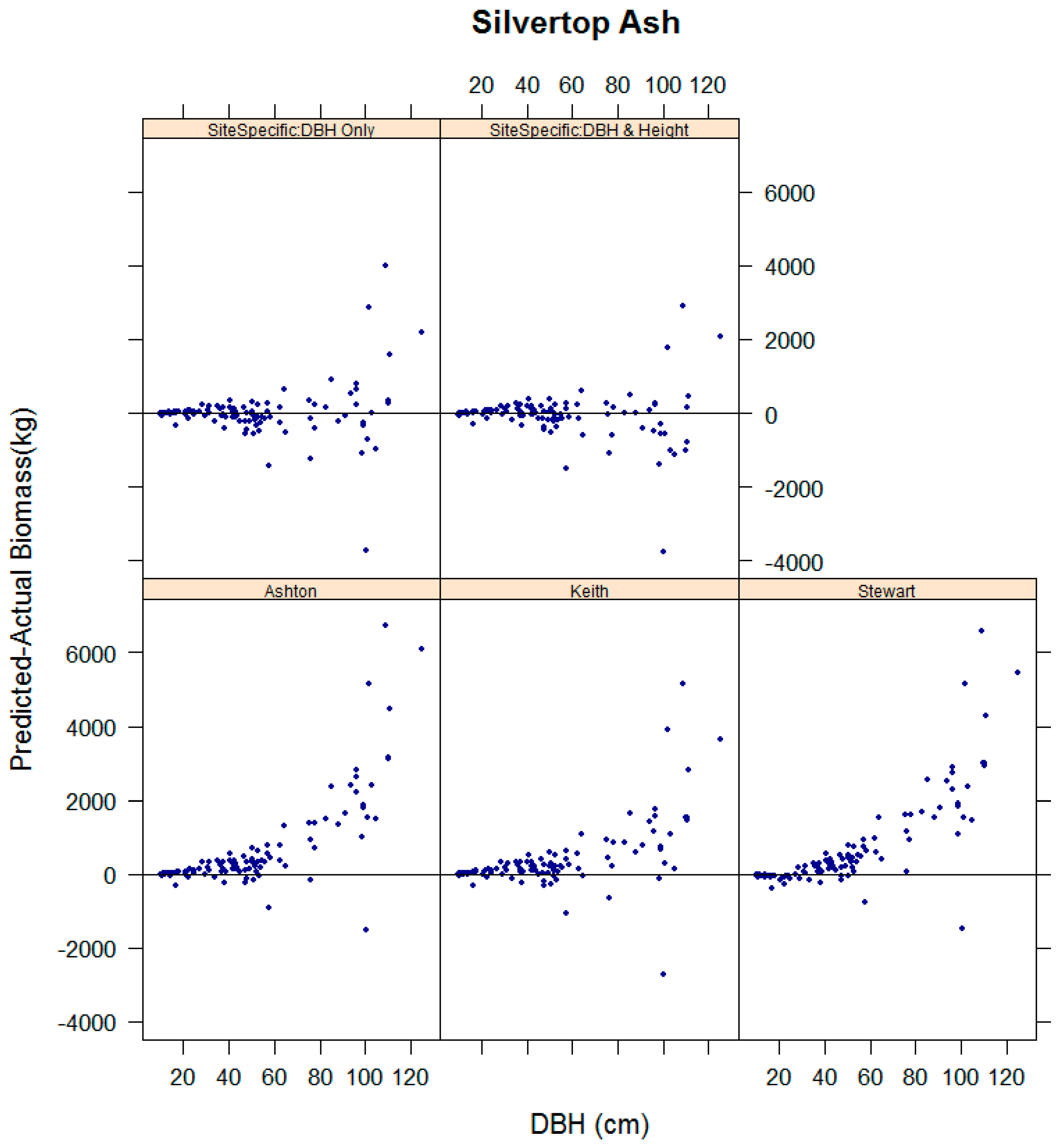
3.4. Evaluation of the Performance of Existing Equations in Estimating Biomass for Key Species in the Study Sites

The performance of the allometric equations listed in Table 5 was compared with that from existing equations for estimating biomass for the key species in the study sites. A number of relevant published allometric equations (Table 2, Methods; Appendix A) were selected and tested against the datasets with actual weights for the three dominant species in this study. This comparison was carried out not with the intention to criticise the selected equations, but rather because they represented, to the best of the authors’ knowledge, the most likely equations to be used for the study sites, in the absence of site-specific equations. A detailed assessment of the development of each of the equations tested to explain any differences between predicted results and those from directly weighed data was outside the scope of this study.
The differences between the model predicted and actual observed AGB values for the three species are presented in Figure 5, Figure 6 and Figure 7. The linear fit of weighed AGBs and the predicted AGB are included in Table 6; a slope value of 1 would indicate a perfect fit.
The published allometric equations for silvertop ash, while reasonable at predicting AGB in the lower DBH range, overestimated the AGB as the DBH increased (Figure 5). In contrast, the selected allometric equations for blackbutt generally underestimated AGB (Figure 6), especially for trees with DBH greater than 40 cm. For mountain ash, AGB estimates varied considerably according to the equation used (Figure 7). Equations by Keith and Ashton [22,26] were very similar and typically resulted in underestimation of biomass for trees with DBH up to approximately 80 cm, and overestimated biomass for larger trees. The equation derived from [28] consistently underestimated AGB, regardless of tree size. Feller’s equation [27] resulted in a large overestimation of AGB regardless of the DBH range (Figure 7)—a similar overestimation was observed by Keith et al. [22], who noted that Feller’s equation was of an unusual form, which appeared to give erroneous values at DBH above 40 cm (Figure 7) [20]. These results were reflected in the very high MAE and bias associated with that relationship (Table 6).

4. Discussion

One of the key components of this study was the direct determination of the AGB of mature native forests stands in Australia. Though comparing AGB between production and conservation sites was less of a focus in this manuscript, the small relative differences between the mountain ash conservation and production sites were noteworthy (Table 4). This may have been partially due to the comparatively smaller differences in age between the production and conservation sites for mountain ash. Although it is difficult to predict how much more AGB a significantly older mountain ash site would sustain, decay would likely become a major factor reducing tree biomass as mountain ash trees mature [20]. Mountain ash is a relatively fast growing species, with some trees less than 70 years old being more than 80 m tall [43], and such rapid growth likely occurs at the expense of fire and decay-resistance [44]. This suggests that the onset of decay is likely to occur relatively early in the mature stage of those stands [20].
The AGB estimates were used to derive AGC in each of the study sites. The AGC estimates for largely undisturbed forests in this study (200–400 t C ha1) are similar to estimates for mature temperate forest types around the world (e.g., 199–586 t C ha1 for temperate forests in North America—[45,46,47]; 146–439 t C ha1 for temperate forests in Chile [48,49]. In the Australian context, Roxburgh et al. [38] calculated tree biomass using the regression equations developed by Ash & Helman [50] and modified to include an adjustment for internal tree decay. The higher AGC reported by Roxburgh et al. [38] refers to the estimated theoretical carbon carrying capacity of the stands, whereas their measured AGC are in agreement with those reported here. The values reported by Turner and Lambert [39] were for fully stocked stands, carrying near maximum biomass when compared with typical stands in the area. AGC reported by Fedrigo et al. [42] for 1939 regrowth mountain ash stands was considerably lower than for the production site in this study of the same age (Figure 2). Their value, however, was in good agreement with the sub-regional estimates provided by the local State Forest agency (VicForests) for pure mountain ash stands in the Central Highlands of Vic (approximately 287 t C/ha) [19]. Keith et al. [41] calculated stem and branch volumes using an allometric equation for mountain ash [28] based on tree diameter (accounting for stem buttressing and internal wood decay), and multiplied by wood density and carbon concentration. There was good agreement between the AGC reported in our study and those in [41] for 1939 regrowth mountain ash stands. However, the productivity of the mountain ash study site was higher than typical 1939 mountain ash regrowth stands. The average AGC suggested by Keith et al. [41] for old-growth mountain ash stands (744 t C ha1) was higher than the AGC for the “conservation” site in this study (415 t C ha1), noting that the old growth stands in [41] were approximately 250-years old. Keith et al. [41] argue that since mountain ash forests may reach ages of 400–500 years, carbon stocks could be higher for those stands. Although trees may continue to grow, albeit slowly, as long as the tree lives [51], this potential increase needs to be countered by the increased levels of decay as trees age. Mountain ash forests at 250 years support typically 20 trees ha1, and a relative decrease in biomass is expected, as the tall open eucalypt forest progresses from aggrading to a steady-state [52]. This suggestion is supported by the findings from Sillett et al. [28], which indicate that decay is a major factor to consider in the estimation of biomass for old-growth mountain ash stands. They estimated biomass in a 0.73 ha plot in Kinglake National Park, VIC, considered by the authors to represent the upper level of the density of large trees for mature mountain ash forests. The maximum estimated AGC was 706 t C ha1; however, the authors noticed extensive decay and numerous hollow trunks and limbs, which they did not take into account for their estimation. If half of the mountain ash heartwood volume was lost to decay, as suggested by [28], AGC in their plot would be reduced to 438 t C ha1. This value is similar to the estimated value for the 1905/1906 mountain ash conservation site from this study (410 t C ha1).
The site-specific biomass data allowed the development and testing of allometric equations based on DBH only, height only, and combined DBH and height. The differences found between the linear equations based on height only for the same species when comparing paired sites may be explained by factors such as site characteristics and stand structure, which is linked to the age of the stands (Appendix C). The results suggest that stand structure for the study regions needs to be factored in before extrapolating the data, as the equations based on height only did vary (Figure 3), even though the mean tree height of the stands did not vary much (Table 3). This is an important factor to consider when using remote sensing techniques (e.g., LiDAR) to derive estimates of variables, such as tree height, which in turn may be used to derive stand volume for large areas.
The combined use of DBH and height as predictive variables for biomass improved the robustness of the simple site-specific DBH only equations, especially when compared to previously published relationships. There are key issues to be considered when evaluating the relative performance of allometric equations, including the method for deriving biomass (i.e., whether directly weighed or derived by sub-sampling), number of trees included and their DBH range, and the impact of potential changes in the nature of the forest over time on the allometry and size of trees. Apart from [23], which included some directly weighed biomass data, all the other equations applied sub-sampling methods to estimate biomass. The number of trees considered in each equation varied considerably, from as few as five trees [26] to over 100 trees [22,23]. Roxburgh et al. [53] suggested that for allometric equations constructed using an adequate size-class distribution of DBH in the population, a minimum sample size of 55 trees for generic Eucalypt species was required. However, this was based on typically younger trees with a smaller DBH range than found in more mature forests—it is expected that the minimum sample size for mature native forest trees to be higher, as they are less uniform and more likely to be impacted by decay.
Over half of the relevant equations for the sites in this study were developed prior to 1990. Although it is unclear whether change in the nature of the forest over time would have resulted in changes in their allometry, this has been identified as one of the potential sources of uncertainty in biomass estimates [13].
Some of the equations were based on significantly younger trees than those included in our study [26,27], and this was also reflected in the lower DBH range for those studies. The impact of tree DBH on biomass derived from allometric equations has been described in a number of studies for both hardwoods and softwoods. Hoover and Smith [54] evaluated a range of biomass equations for US temperate forests. They found that while most equations returned similar estimates for trees up to 50 cm DBH, equation behavior diverged at larger diameters, in some cases returning estimates that were considerably different. Bragg [18] described similar results for loblolly pine (Pinus taeda L.) after testing four existing allometric equations for that species. However, it was not possible to determine which model was closer to reality as the large live trees were not destructively sampled, highlighting the challenges of assessing the accuracy of biomass estimation for large trees when models that include directly weighed data for such large trees do not exist. The large stand-level discrepancies demonstrated by [18] when using different equations calls into question large-scale carbon storage estimates based on equations that have not been properly evaluated and/or are stretched beyond their intended range. Duncanson et al. [55] demonstrated that small sample sizes and the under-representation of large trees are the key reasons for the overestimation of biomass in some models used to predict biomass in tropical forests.

5. Recommendations for Further Research

Currently, there is a limited understanding on minimum sample sizes required for the development of allometric equations for trees in mature stands. The dataset generated in this study will be used to investigate this further and will be included in a future manuscript.
Although recent advances in LiDAR technologies (e.g., ground-based LiDAR) in obtaining highly precise estimates of individual tree volumes may reduce the need for the destructive sampling of trees in future [55], this does not take into consideration the impact of internal decay on biomass estimations. Decay is an important factor to consider in biomass estimations of mature trees. There is considerable uncertainty about the patterns of decay onset for different native forest species, and importantly, its impact on biomass loss as the trees grow older [20]. Decay in mature forests may be correlated to age, species, basal area, presence of biological hazards, and management interventions (e.g., thinning)—these relationships need to be examined further [20]. It may be possible to combine the application of LiDAR techniques with techniques that can be used to estimate decay in standing mature trees. These may include, for example, the use of acoustic tomography combined with modified micro-drilling, as demonstrated by Wang and Alisson [56] for 200-year old red oak (Quercus rubra L.) trees in Wisconsin, USA. This is the area of mature forest biomass research that would potentially result in the biggest contribution towards reducing current uncertainties in forest biomass and carbon estimates.

6. Conclusions

In this study, we weighed a large number of trees in order to determine biomass for mature native forests managed for periodic cycles of harvest or conservation only, and used the data to propose new allometric equations and to test the robustness of existing allometric equations in estimating biomass.
Direct weighing of biomass ensured a degree of certainty in the results that cannot be associated with previous studies that relied on sub-sampling, or with studies that relied on existing allometric equations, which typically do not include the range of sizes that exist in mature native forests. We demonstrated that the use of existing allometric equations for the relevant species in this study is unreliable and generally poor at estimating biomass for mature trees. Thus, biomass and carbon estimates for large areas of forests based on allometric equations that have not been shown to be reliable across different geographical areas should be avoided. Adding the new data on large trees presented here to existing allometric equations where relevant may help to reduce their bias and refine predictions.
Total AGC was high but not as high as previously claimed for some SE forests in Australia—previous studies that did not rely on direct weighing of the biomass significantly overestimate that potential for the forests included in this study. Thus, caution should be exercised when interpreting the results of such studies in the context of decisions around optimum forest management regimens and the contribution of mature forest stands to the global carbon balance.

Acknowledgments

We acknowledge the contributions from Tim Parkes, Justin Crowe, and Shane Clohesy (Forestry Corporation of NSW) for region-specific information on the forest types, yields, and product mixes. We thank Simon Murphy and Tarek Murshed (University of Melbourne), and Graeme Mitchell and Tom Goldstraw (VicForests) for assistance in the field for the Victorian work, and Mirella Peters for assistance with setting up plots. We thank Forests and Wood Products Australia (FWPA) for the financial support provided.

Author Contributions

Fabiano A. Ximenes conceived and designed the study; Michael MacLean, Rebecca Coburn, David Sargeant, Matthew Mo, and Fabiano A. Ximenes performed the study and managed the data; Amrit Kathuria carried out the statistical analyses of the data; Justin Williams, Michael Ryan, and Ken Boer provided operational support and input into plot selection; Fabiano Ximenes wrote the paper with contributions from Rebecca Coburn, Michael MacLean, and Amrit Kathuria.

Conflicts of Interest

The authors declare no conflict of interest.

Appendix A. Site Details

A more complete description of the study sites can be found in [20]—a summary of the information is included below.

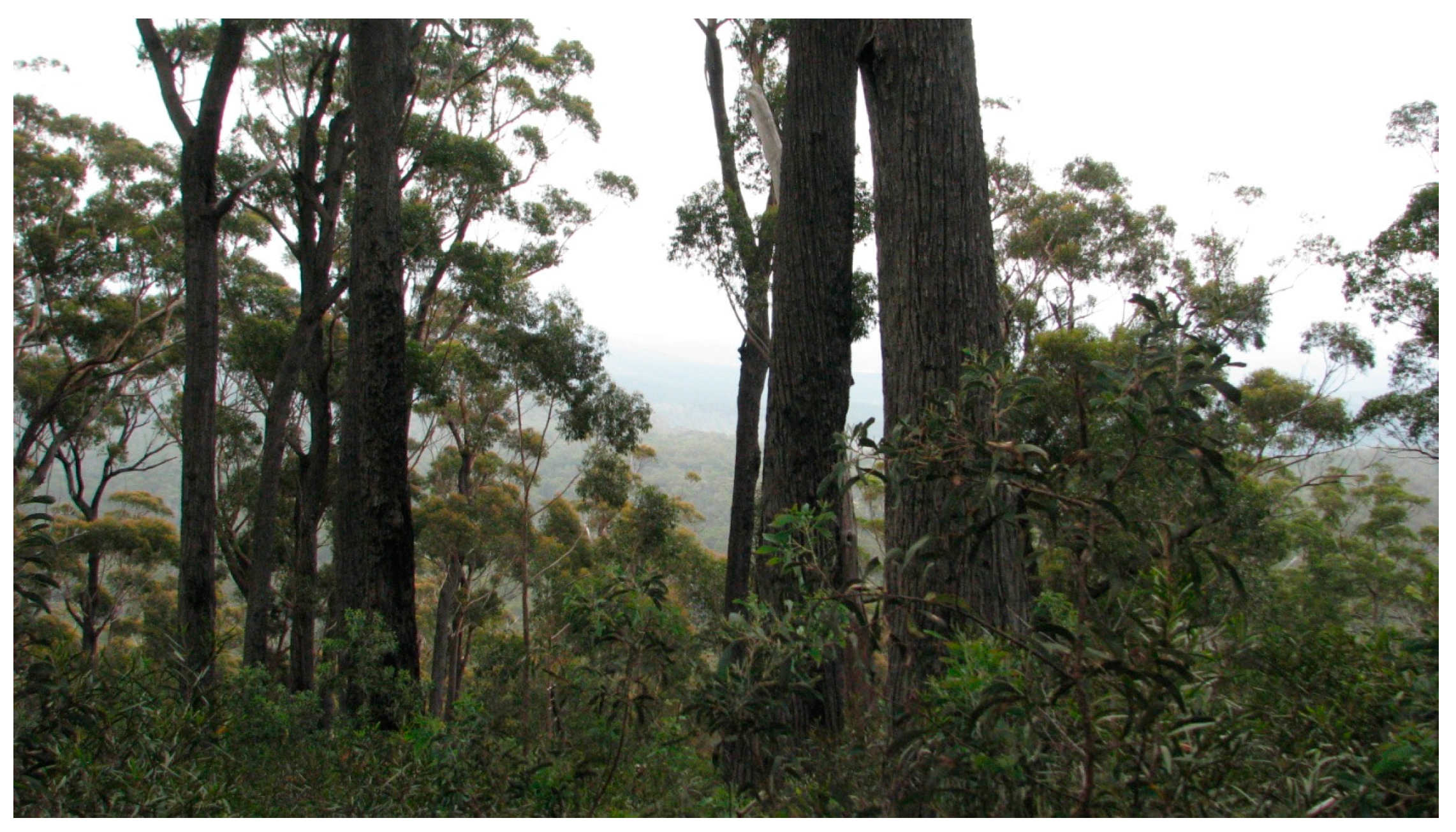
Appendix A.1. NSW South Coast—Eden—Silvertop Ash

The paired NSW South Coast biomass sites were located at Yambulla State Forest, approximately 30 km south west of Eden. They were located approximately 2 km apart in compartments 500 (production site) and 501 (conservation site).

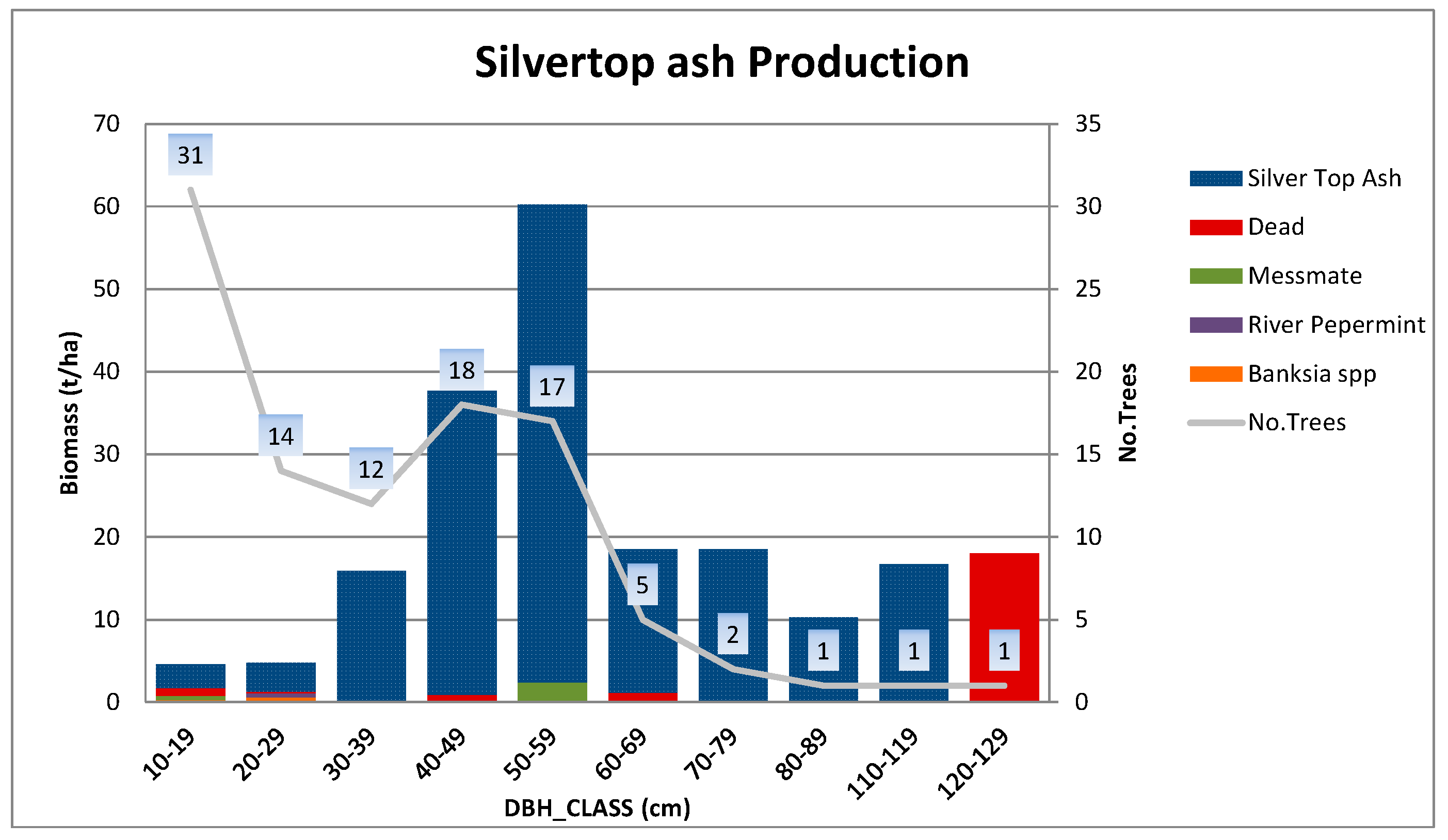
Appendix A.1.1. Silvertop Ash Production Site

The production site was located on a relatively level, sandy area on the south side of Black Range Rd (149°40′42.57″ E 37°8′10.92″ S), with most trees being regrowth from approximately 1950 (Figure A1). The dominant species was silvertop ash with occasional yellow stringybark (Eucalyptus muellerana A.W. Howitt.) and narrow leaf peppermints (Eucalyptus radiata Sieb, ex DC subsp. radiata). Shrub cover was mostly made up of saw banksia and wattle, while groundcover was sparse to moderately covered with ferns and grasses. There was evidence of past bushfires and harvest. The site was in a compartment which was scheduled for harvest as part of FCSNW Eden harvest operations.
Figure A1. Overview of the silvertop ash “production” site.
Forests 09 00060 g0a1

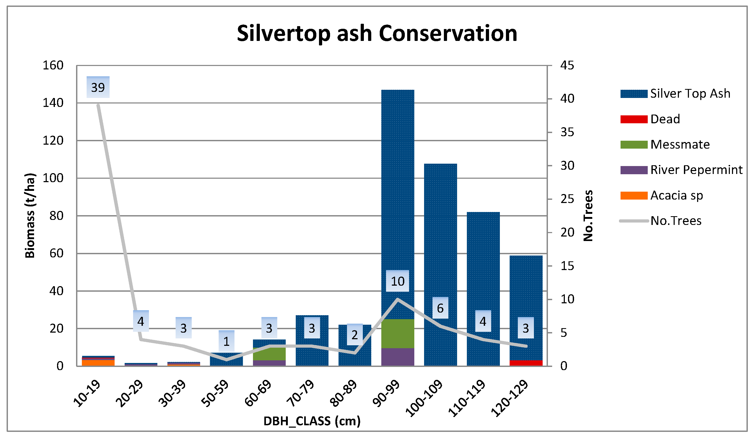
Appendix A.1.2. Silvertop Ash Conservation Site

The conservation site (Figure A2) was located on a north-western facing rocky ridgetop and upper slope off Skink Rd (149°41′30.14″ E 37°8′42.99″ S). The site contained a number of mature trees with DBH > 100 cm. The forest was dominated by silvertop ash, with occasional river peppermint (Eucalyptus elata Dehnh.) and messmate (Eucalyptus obliqua L’Hér). Shrubcover was dominated by Acacia sp. and groundcover by ferns. The forest was 200–250+ years for the older/dominant cohort and 60–70 years for the second cohort.
Figure A2. Overview of the silvertop ash “conservation” site.
Forests 09 00060 g0a2

Appendix A.2. NSW North Coast—Wauchope—Blackbutt

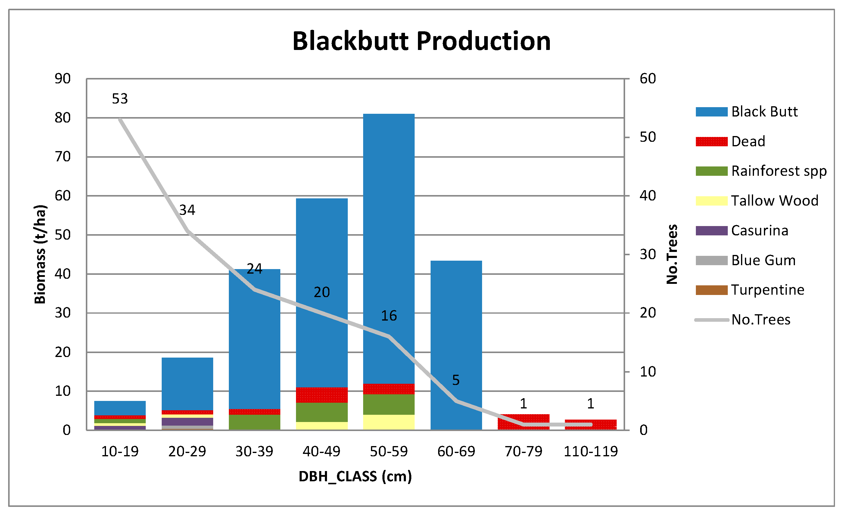
Appendix A.2.1. Blackbutt Production Site

The blackbutt production site was located on a south-west facing slope, in a harvest area at the end of Mcmillians Rd (152°25′36.08″ E 31°13′50.15″ S) in Mt Boss State Forest (Figure A3). Most trees were regrowth from approximately the 1950’s (Figure A3). The dominant species was blackbutt with occasional tallowwood (Eucalyptus microcorys F. Muell) and Sydney blue gum (Eucalyptus saligna Sm.). Shrub cover was mostly made up of casuarina, wattle, and rainforest species. Groundcover was medium to heavily covered with vines and grasses. There was some evidence of past bushfires and harvest with many large stumps and charred harvest slash present. The site was in a compartment which was scheduled for harvest as part of FCNSW Central region harvest operations.
Figure A3. Blackbutt production site (a) Before harvest (b) Post-harvest.
Forests 09 00060 g0a3

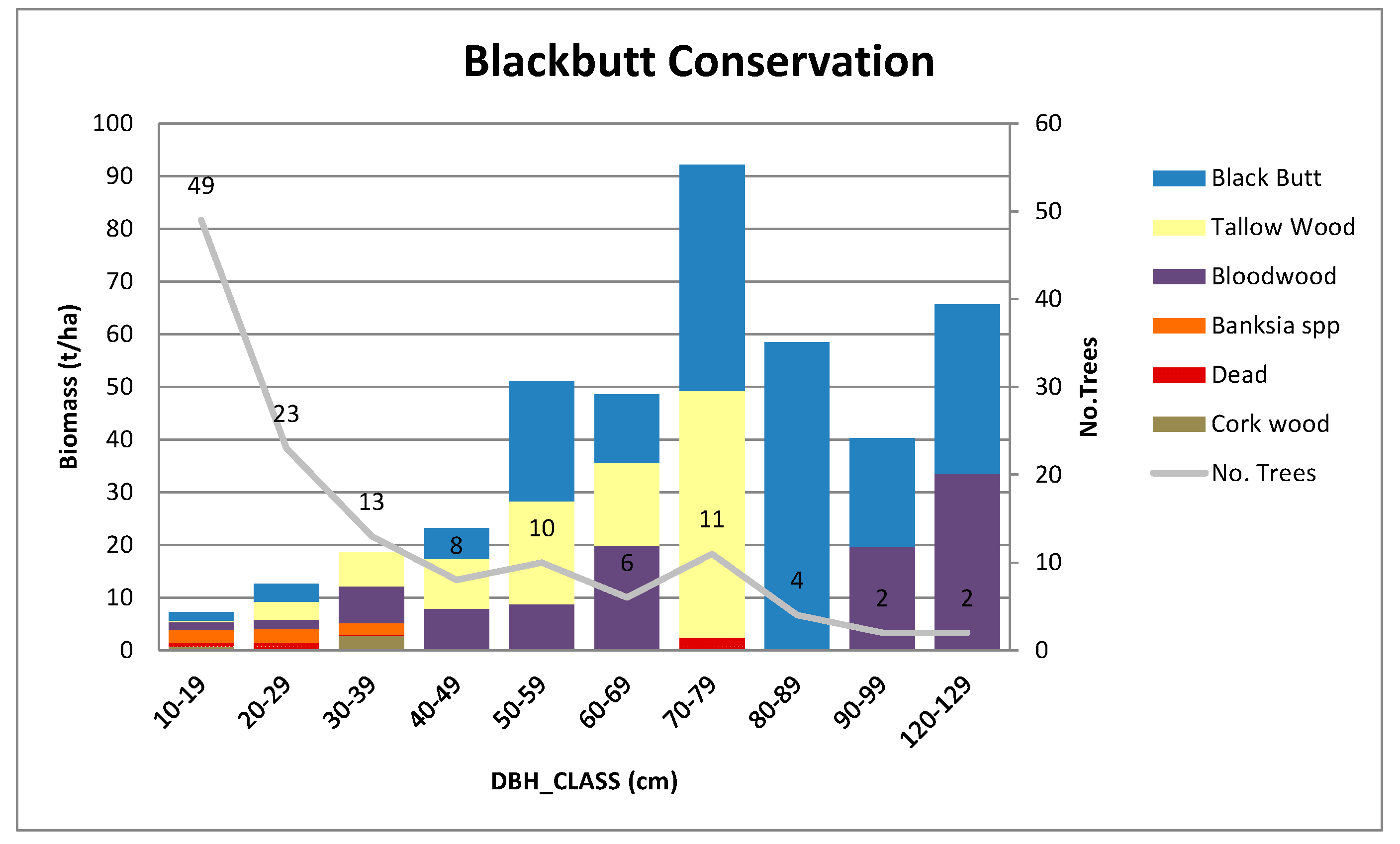
Appendix A.2.2. Blackbutt Conservation Site

The blackbutt conservation site was located on a flat terrain, sandy area (152°48′44.35″ E 31°37′17.45″ S) 5 km north of village of North Haven (Figure A4). The stand was relatively untouched from forest management. The dominant species was blackbutt, with red bloodwood and tallowwood co-dominating. Shrub cover was mostly made up of saw banksia (and corkwood). Groundcover was medium to heavy cover with ferns and grasses. Although there was evidence of past bushfires, the site had not been burnt recently. The site was in a compartment which was approved for harvest as part of private native forest harvest operations with the Bunyah Local Aboriginal Lands Council. It was a multi-aged stand—the large bloodwood and blackbutt trees were >200 years old, and the 60–100 cm blackbutt probably circa 1920–30s.
Figure A4. Blackbutt forest: (a) Before harvest—largest blackbutt; (b) Harvest of plot; (c) post-harvest.
Forests 09 00060 g0a4

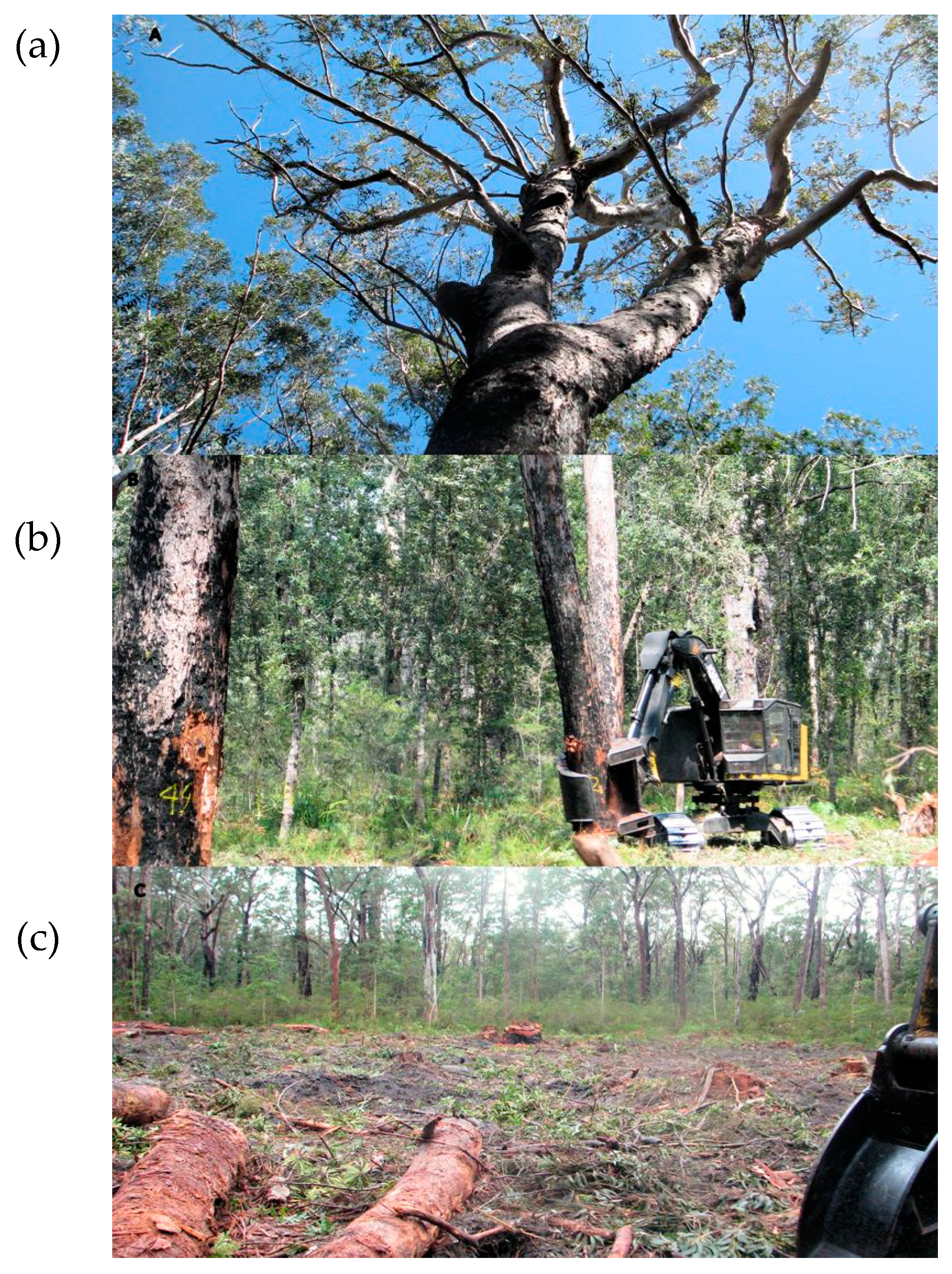
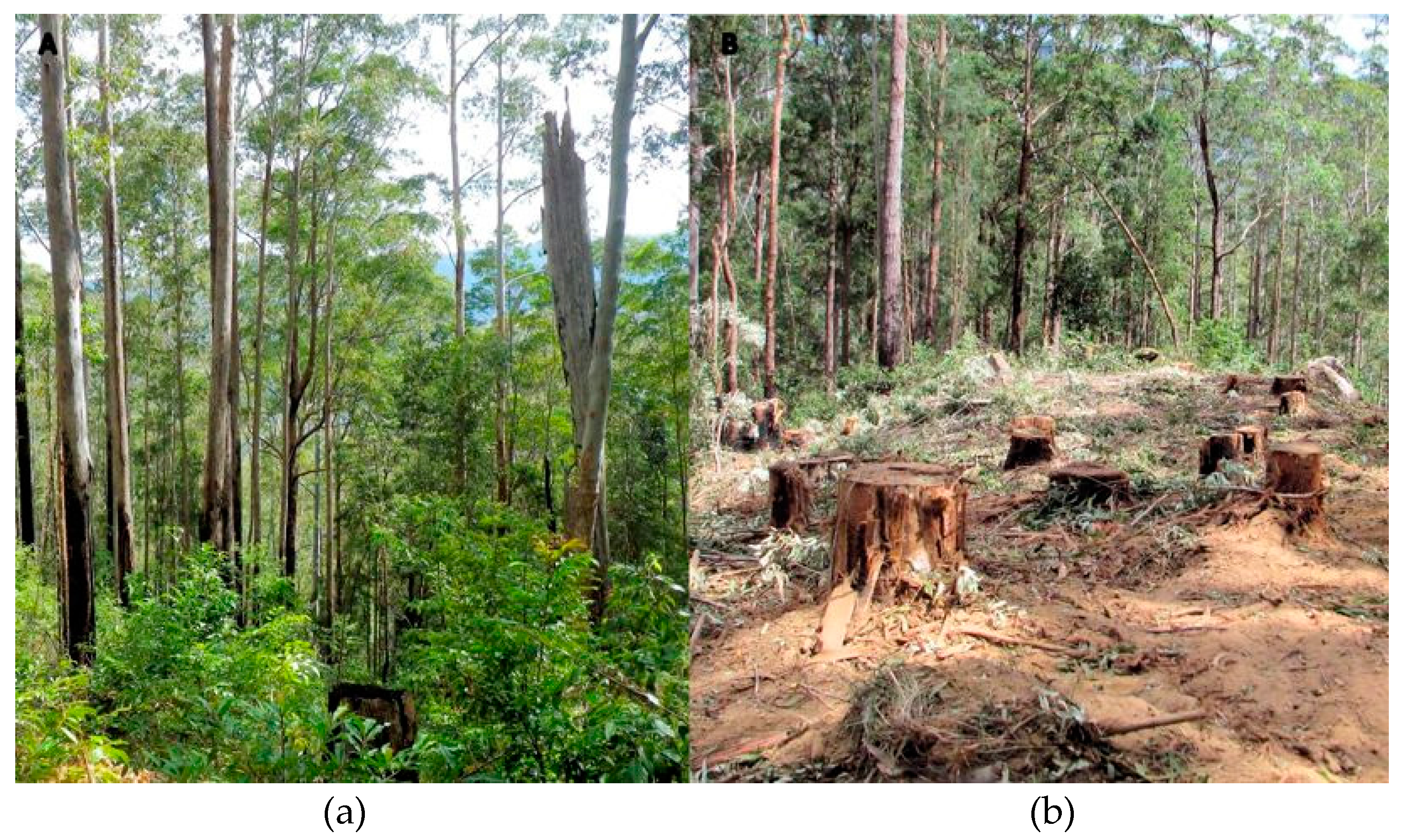
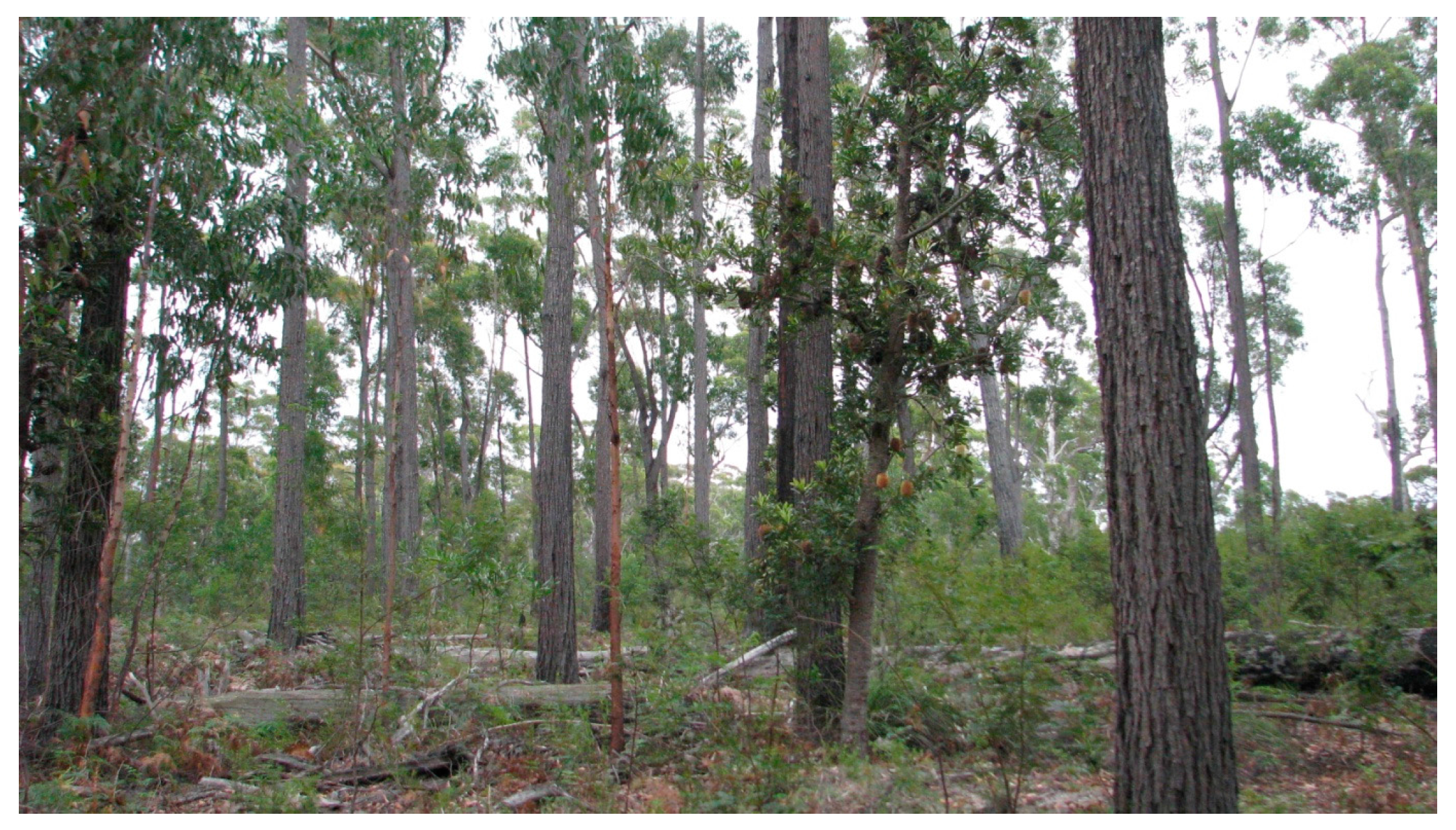
Appendix A.3. VIC Central Highlands—Mountain Ash

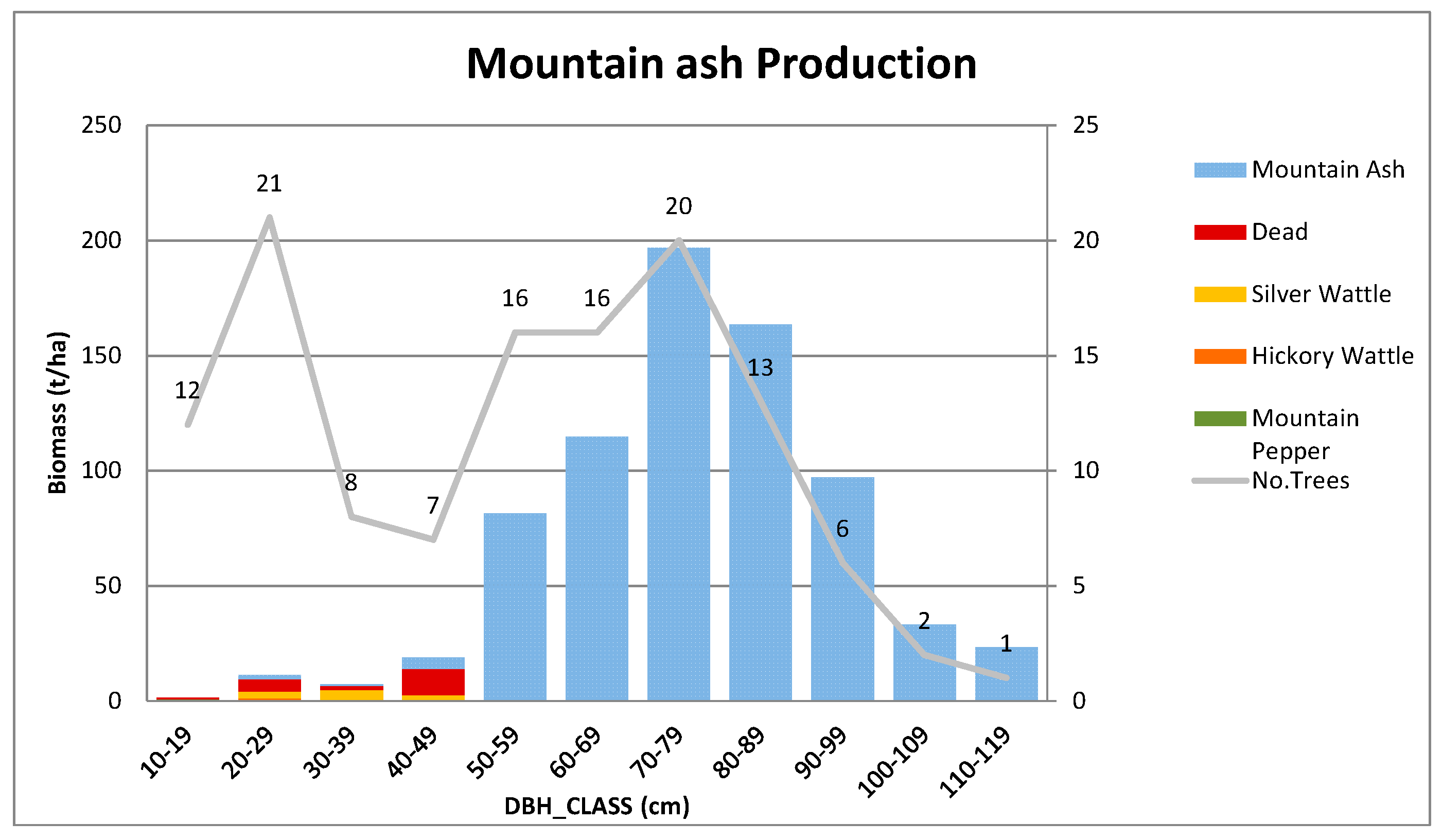
Appendix A.3.1. Mountain Ash Production Site

The Victorian mountain ash production site was located at Toolangi SF, approximately 30 km north of Healesville (145°32′43.41″ E 37°31′46.00″ S). The mountain ash production site was located on an east facing slope, in a harvest area at the end of Hardy Creek Rd, with most trees being regrowth from 1939 fire (Figure A5). The dominant species was mountain ash with a sub canopy of silver wattle (Acacia dealbata subsp. dealbata), hickory wattle (Acacia obliquinervia Desv.), and mountain pepper (Tasmannia lanceolata (Poir.) A.C.Sm.). Shrub cover was mostly made up of Correa spp. and tree ferns. Groundcover was light with a heavy mulch layer around live trees. There was little evidence of past bushfires. There was evidence of past harvest with a few small rotten stumps from a thinning event. The site was in a compartment which was scheduled for harvest as part of VicForests harvest operations.
Figure A5. Mountain ash forest: (a) Before harvest; (b) Weighing mountain ash on trailer; (c) post-harvest.
Forests 09 00060 g0a5

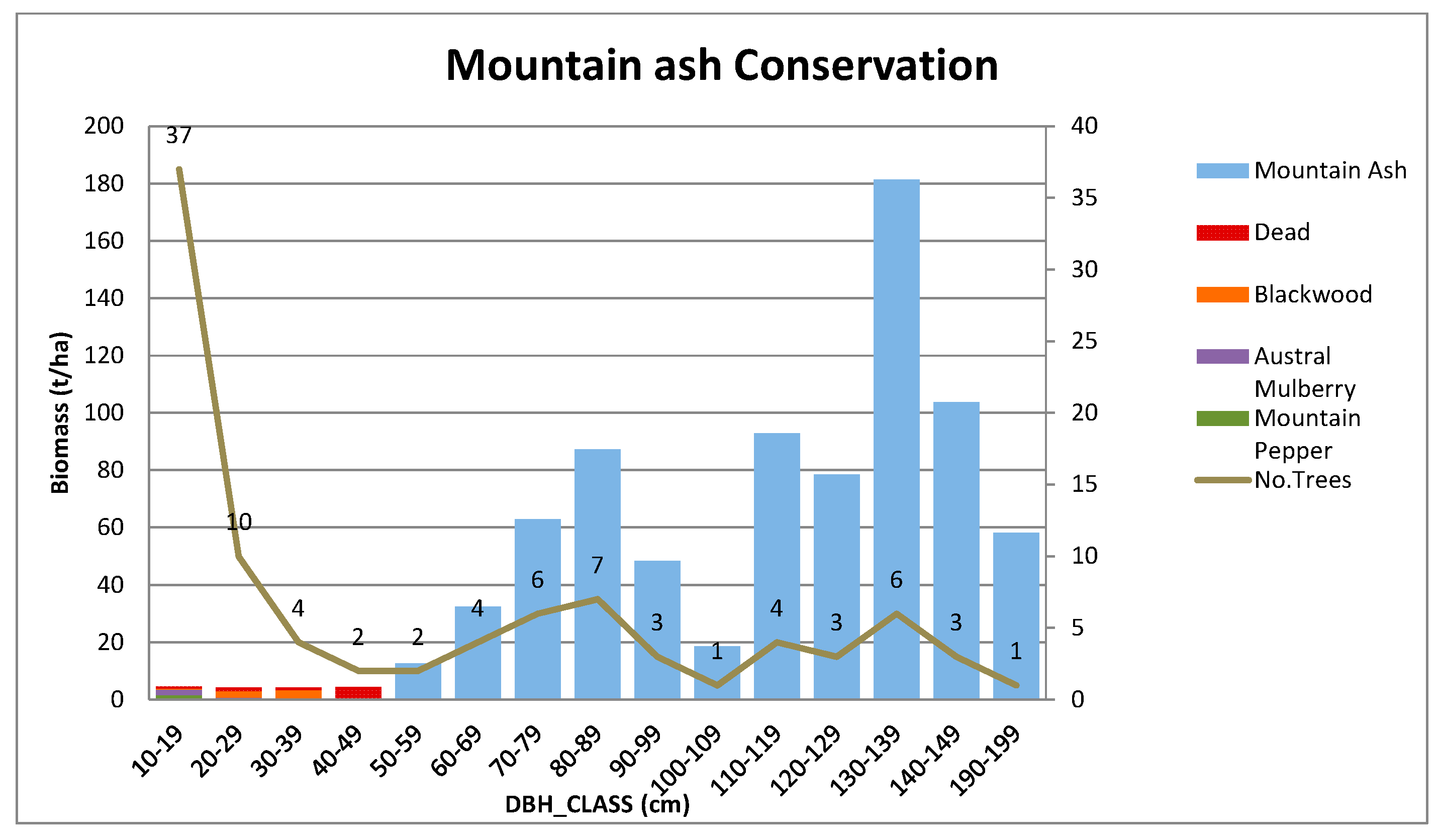
Appendix A.3.2. Mountain Ash Conservation Site

It was not possible to directly weigh biomass from a significantly older mountain ash site for use as the conservation scenario for Victoria. An alternative approach was followed, where a 0.5 ha plot was established at the “Gun Barrel” coupe (145°30′54.35″ E 37°30′23.69″ S), which contained a number of trees with DBH significantly greater than those at the production site, due to the stand being primarily regrowth from the 1905/06 fire. Every tree with a DBH greater than 10 cm was measured. The biomass information derived from both the “production” site and from a number of additional large trees identified around the production site was used to derive allometrics employed to estimate biomass in the measured trees from the “Gun Barrel” coupe.

Appendix B. Moisture and Density of Tree Components and AGB by DBH Class

Appendix B.1. Method for Determining Moisture Content and Basic Density of Biomass Components

The methods for determining moisture content and basic density are described in detail in [20]. Samples of the various tree components were taken from a selection of trees from each site (Table A1), ensuring that a range of species and DBH classes were represented [20].
Table A1. Number of samples of tree components used for moisture content and basic density determinations.
Tree ComponentSpecies
BlackbuttSilvertop AshMountain AshTotal
Stem (lower part–stump)385025113
Stem (middle part)24284294
Stem (upper part)40372097
Bark837051204
Branches13161339

Appendix B.2. Moisture Content and Basic Density of Biomass Samples

In Table A2, the moisture content and basic density for a range of tree biomass fractions for the key species in the study sites is included. Analyses of the results can be found in [20].
Table A2. Moisture content and basic density for the various biomass fractions of key species in each study region.
SiteStatusStumpStemCrown 1Bark
MC (%)BD (kg/m3)MC (%)BD (kg/m3)MC (%)BD (kg/m3)MC (%)BD (kg/m3)
BlackbuttRegrowth43 (5)660 (61)41 (3)663 (52)39 (4)661 (67)56 (6)377 (56)
BlackbuttMature38 (3)766 (44)37 (3)767 (58)35 (4)783 (61)57 (4)416 (45)
Mountain ashRegrowth57 (3)474 (43)49 (4)533 (45)44 (7)567 (55)60 (5)380 (39)
Silvertop ashRegrowth46 (4)633 (72)41 (3)671 (34)40 (4)678 (57)46 (7)541 (68)
Silvertop ashMature46 (5)635 (85)39 (2)688 (43)38 (6)679 (71)46 (8)523 (121)
1 The moisture content and basic density for the crown is the mathematical average of the moisture content of crown discs and branches. The bark was not removed from the branch component, thus the moisture content and basic density for the branch includes the branch bark.

Appendix B.3. Standing Above-Ground Biomass (AGB)—Contribution by DBH Class

The proportion of the AGB represented by the various DBH classes for each study site is represented in Figure A6, Figure A7, Figure A8, Figure A9, Figure A10 and Figure A11 [20]. The high number of understorey and/or regrowth trees in the 10–19 cm range contributed very little to the AGB (Figure A6, Figure A7, Figure A8, Figure A9, Figure A10 and Figure A11). The dominant species accounted for the majority of the AGB in the study sites (88–90% for silvertop ash, 48–83% for blackbutt, and 99% for mountain ash production site). Past bushfires in the silvertop ash and blackbutt conservation sites have likely contributed to the multi-aged profile of the stands (Figure A7 and Figure A9). The mountain ash conservation site was comprised of two distinct age classes as shown in the bimodal pattern in Figure 1f, which is consistent with the bushfire history for that site [20].
For the production sites, the AGB was concentrated in the DBH classes targeted for commercial extraction (48–54% of the biomass in the DBH range of 40–59 cm for silvertop ash and blackbutt and 70–79 cm for mountain ash), (Figure A6, Figure A8 and Figure A10). For the conservation sites, the AGB was concentrated on trees with larger DBH (Figure A7, Figure A9 and Figure A11).
Figure A6. The distribution of AGB and number of trees across the DBH classes for the silvertop ash production site.
Forests 09 00060 g0a6
Figure A7. The distribution of AGB and number of trees across the DBH classes for the silvertop ash conservation site.
Forests 09 00060 g0a7
Figure A8. The distribution of AGB and number of trees across the DBH classes for the blackbutt production site.
Forests 09 00060 g0a8
Figure A9. The distribution of AGB and number of trees across the DBH classes for the blackbutt conservation site.
Forests 09 00060 g0a9
Figure A10. The distribution of AGB and number of trees across the DBH classes for the mountain ash production site.
Forests 09 00060 g0a10
Figure A11. The distribution of AGB and number of trees across the DBH classes for the mountain ash conservation site. Please note that the biomass was not directly weighed but rather derived from a biomass relationship derived from mountain ash trees weighed in the vicinity of this forest.
Forests 09 00060 g0a11

Appendix C. Further Details on Allometric Equations Used in This Study

Here, a summary of the underlying information associated with each of the allometric equations tested is included, with the information originally contained in [20].
Table A3. Description of how the various DBH: biomass relationships tested in this study were derived.
SourceDescription of Equation Development
Montagu et al. [23]Montague et al. [23] derived a number of equations specifically for blackbutt across seven study sites (five in the central and north coast of NSW and two at Fraser Island, Queensland), including plantations and native forests—we used the general DBH equation which was fitted across all study sites (DBH range 5–129 cm) without a correction factor. The biomass estimates were based on a mix of direct measurements of the fresh mass of the entire tree and subsampling techniques to estimate the biomass of tree components.
Mackowski [24]Mackowski [24] proposed a number of equations for blackbutt with specific DBH ranges, derived for blackbutt-dominated forests 30–40 km south east of Grafton, NSW, based on measurements of ninety trees with DBH up to 189.6 cm—we used the equation for a DBH range of 45–135 cm [22]. Stem and branch volume were estimated using a log volume formula, with biomass estimated using published density values
Applegate [25]Applegate [25] derived a number of equations based on blackbutt biomass data collected from Fraser Island, Queensland—we used the regeneration old growth equation which covered a DBH range of 13–129 cm [22]. Twenty-nine large trees ranging from 12.2 to 128.9 cm were felled; however the DBH class distribution was limited with only one tree with DBH greater than 60 cm (128.9 cm). The branches and foliage of each tree were weighed in the field for all but the large tree and samples taken for dry weight determinations. Biomass for the stem was calculated for logs based on the volume of the sapwood, heartwood and bark and density determinations.
Ashton [26]Equation developed for silvertop ash and mountain ash (both study sites in Victoria). It was based on five 27-year old silvertop ash trees which were felled, with branches and leaves weighed in the field and stem biomass estimated from volume and physical parameters derived from stem discs.
Feller [27]DBH and height equation developed specifically for mountain ash located at the Maroondah catchment area (State of Victoria), based on destructive sampling of six trees of varying size (four trees ranging from 15 to 30 cm DBH, one around 50 cm and the largest one around 70 cm DBH). The biomass of the crown was derived by a combination of determining the moisture content of a sub-sample of smaller diameter branches, and the use of published density values for the measured larger diameter branches. The biomass of the stem was also calculated based on published density values and stem measurements.
Stewart et al. [29]Additive equation developed specifically for silvertop ash, in the State of Victoria. They sampled ten silvertop ash with DBH ranging between 28 and 89 cm, with the larger trees being more than 100-year old. The diameter of the stem and branches from every tree was measured, and biomass estimated based on destructive sampling of a sub-set of stem discs and branch samples of varying sizes.
Silett et al. [28] (derived)Equation derived using their published biomass data for 22 trees with a DBH range of 80–312 cm, located at Kinglake National Park, VIC [40]. The biomass estimates were based on detailed field measurements (especially of the crown component), with subsampling techniques used to estimate the biomass of tree components.
Keith et al. [22]Generic equation for native sclerophyll forests (including for the key species in this study), based on 25 records and 135 data points, with biomass of individual trees calculated for trees with DBHs ranging from 10 to 100 cm DBH (10 cm increments).

References

  1. Canadell, J.G.; Raupach, M.R. Managing forests for climate change mitigation. Science 2008, 320, 1456–1457. [Google Scholar] [CrossRef] [PubMed]
  2. Intergovernmental Panel on Climate Change (IPCC). Chapter 3, Section 3.2 Forest Land. In Good Practice Guidance for LULUCF; Nabuurs, G., Ravindranath, N.H., Paustian, K., Freibauer, A., Hohenstein, W., Makundi, W., Eds.; IPCC National Greenhouse Gas Inventories Programme: Hayama, Japan, 2003; Available online: http://www.ipcc-nggip.iges.or.jp/public/gpglulucf/gpglulucf_files/Chp3/Chp3_2_Forest_Land.pdf (accessed on 02 March 2017).
  3. Intergovernmental Panel on Climate Change (IPCC). Revised Supplementary Methods and Good Practice Guidance Arising from the Kyoto Protocol; Hiraishi, T., Krug, T., Tanabe, K., Srivastava, N., Baasansuren, J., Fukuda, M., Troxler, T.G., Eds.; IPCC: Geneva, Switzerland, 2014. [Google Scholar]
  4. Available online: https://www.montrealprocess.org/documents/publications/techreports/MontrealProcessSeptember2015.pdf (accessed on 13 December 2017).
  5. Bellassen, V.; Luyssaert, S. Managing forests in uncertain times. Nature 2014, 506, 153–155. [Google Scholar] [CrossRef] [PubMed]
  6. Krankina, O.N.; Harmon, M.E.; Schnekenburger, F.; Sierra, C.A. Carbon balance on federal forest lands of Western Oregon and Washington: The impact of the Northwest Forest Plan. For. Ecol. Manag. 2012, 286, 171–182. [Google Scholar] [CrossRef]
  7. Colombo, S.J.; Chen, J.; Ter-Mikaelian, M.T.; McKechnie, J.; Elkie, P.C.; MacLean, H.L.; Heath, L.S. Forest protection and forest harvest as strategies for ecological sustainability and climate change mitigation. For. Ecol. Manag. 2012, 281, 140–151. [Google Scholar] [CrossRef]
  8. Hennigar, C.R.; MacLean, D.A.; Amos-Binks, L.J. A novel approach to optimize management strategies for carbon stored in both forests and wood products. For. Ecol. Manag. 2008, 256, 786–797. [Google Scholar] [CrossRef]
  9. Klein, D.; Hollerl, S.; Blaschke, M.; Schulz, C. The contribution of managed and unmanaged forests to climate change mitigation—A model approach at stand level for the main tree species in Bavaria. Forests 2013, 4, 43–69. [Google Scholar] [CrossRef]
  10. Keith, H.; Lindenmayer, D.; Macintosh, A.; Mackey, B. Under what circumstances do wood products from native forests benefit climate change mitigation? PLoS ONE 2015, 10, e0139640. [Google Scholar] [CrossRef] [PubMed]
  11. Ximenes, F.; George, B.H.; Cowie, A.; Williams, J.; Kelly, G. Greenhouse gas balance of native forests in New South Wales, Australia. Forests 2012, 3, 653–683. [Google Scholar] [CrossRef]
  12. Lefsky, M.A.; Cohen, W.B.; Parker, G.G.; Harding, D.J. LiDAR remote sensing for ecosystem studies. BioScience 2002, 52, 19–30. [Google Scholar] [CrossRef]
  13. Brown, S. Measuring carbon in forests: Current status and future challenges. Environ. Pollut. 2002, 116, 363–372. [Google Scholar] [CrossRef]
  14. Clark, D.B.; Kellner, J.R. Tropical forest biomass estimation and the fallacy of misplaced concreteness. J. Veg. Sci. 2012, 23, 1191–1196. [Google Scholar] [CrossRef]
  15. Chave, J.; Condit, R.; Aguilar, S.; Hernandez, A.; Lao, S.; Perez, R. Error propagation and scaling for tropical forest biomass estimates. Philos. Trans. R. Soc. Lond. B. Biol. Sci. 2004, 359, 409–420. [Google Scholar] [CrossRef] [PubMed]
  16. Van Breugel, M.; Ransijn, J.; Craven, D.; Bongers, F.; Hall, J.S. Estimating carbon stock in secondary forests: Decisions and uncertainties associated with allometric biomass models. For. Ecol. Manag. 2011, 262, 1648–1657. [Google Scholar] [CrossRef]
  17. Picard, N.; Laurent, S.-A.; Henry, M. Manual for Building Tree Volume and Biomass Allometric Equations: From Field Measurement to Prediction; Food and Agricultural Organization of the United Nations, Rome and Centre de Cooperation Internationale en recherche Agronomique pur le Developpement: Montpellier, France, 2012. [Google Scholar]
  18. Bragg, D.C. Modeling loblolly pine aboveground live biomass in a mature pine-hardwood stand: A cautionary tale. J. Ark. Acad. Sci. 2011, 65, 31–38. [Google Scholar]
  19. Keith, H.; Mackey, B.; Lindenmayer, D. Re-evaluation of forest biomass carbon stocks and lessons from the world’s most carbon-dense forests. Proc. Natl. Acad. Sci. USA 2009, 106, 11635–11640. [Google Scholar] [CrossRef] [PubMed]
  20. Ximenes, F.; Roxburgh, S.; Cameron, N.; Coburn, R.; Bi, H. Carbon Stocks and Flows in Native Forests and Harvested Wood Products in SE Australia. Report Prepared for Forest and Wood Products Australia. 2016. Available online: http://www.fwpa.com.au/images/resources/Amended_Final_report_C_native_forests_PNC285-1112.pdf (accessed on 03 May 2017).
  21. Ximenes, F.A.; Gardner, W.D.; Kathuria, A. Proportion of above-ground biomass in commercial logs and residues following the harvest of five commercial forest species in Australia. For. Ecol. Manag. 2008, 256, 335–346. [Google Scholar] [CrossRef]
  22. Keith, H.; Barrett, D.; Keenan, R. Review of Allometric Relationships for Woody Biomass for NSW, ACT, VIC, TAS, SA; National C Accounting Technical Report No. 5b; Australian Greenhouse Office: Canberra, Austrilia, 2000. [Google Scholar]
  23. Montagu, K.D.; Duttmer, K.; Barton, C.V.M.; Cowie, A.L. Developing general allometric relationships for regional estimates of carbon sequestration—An example using Eucalyptus pilularis from seven contrasting sites. For. Ecol. Manag. 2005, 204, 113–127. [Google Scholar] [CrossRef]
  24. Mackowski, C.M. Wildlife Hollows and Timber Management in Blackbutt Forest. Master’s Thesis, University of New England, Armidale, Australia, 1987. [Google Scholar]
  25. Applegate, G.B. Biomass of Blackbutt (Eucalyptus pilularis Sm.) Forests on Fraser Island. Master’s Thesis, University of New England, Armidale, Australia, 1982. [Google Scholar]
  26. Ashton, D.H. Phosphorus in forest ecosystems at Beenak, Victoria. J. Ecol. 1976, 64, 171–186. [Google Scholar] [CrossRef]
  27. Feller, M.C. Biomass and nutrient distribution in two Eucalypt forest ecosystems. Aust. J. Ecol. 1980, 5, 309–333. [Google Scholar] [CrossRef]
  28. Sillett, S.C.; van Pelt, R.; Kramer, R.D.; Carroll, A.L.; Koch, G.W. Biomass and growth potential of Eucalyptus regnans up to 100 m tall. For. Ecol. Manag. 2015, 348, 78–91. [Google Scholar] [CrossRef]
  29. Stewart, H.T.L.; Flinn, D.W.; Aeberli, B.C. Aboveground biomass of a mixed Eucalypt forest in eastern Victoria. Aust. J. Bot. 1979, 27, 725–740. [Google Scholar] [CrossRef]
  30. Tukey, J.W. We need both exploratory and confirmatory. Am. Stat. Assoc. 1980, 34, 23–25. [Google Scholar]
  31. Jolliffe, I.T.; Stephenson, D.B. Forecast Verification: A Practitioner’s Guide in Atmospheric Science; Wiley & Sons: New York, NY, USA, 2003; 240p. [Google Scholar]
  32. Nash, J.E.; Sutcliffe, J.V. River flow forecasting through conceptual models Part I—A discussion of principles. J. Hydrol. 1970, 10, 282–290. [Google Scholar] [CrossRef]
  33. R Core Team. R: A Language and Environment for Statistical Computing; R Foundation for Statistical Computing: Vienna, Austria, 2015; Available online: http://www.R-project.org/ (accessed on 05 May 2017).
  34. Venables, W.N.; Ripley, B.D. Modern Applied Statistics with S, 4th ed.; Springer: New York, NY, USA, 2002; ISBN 0-387-95457-0. [Google Scholar]
  35. Zambrano-Bigiarini, M. hydroGOF: Goodness-of-Fit Functions for Comparison of Simulated and Observed Hydrological Time Seriesr Package Version 0.3-10. 2017. Available online: http://hzambran.github.io/hydroGOF/ (accessed on 05 May 2017). [CrossRef]
  36. Wickham, H. Ggplot2: Elegant Graphics for Data Analysis; Springer: New York, NY, USA, 2009. [Google Scholar]
  37. Sarkar, D. Lattice: Multivariate Data Visualization with R; Springer: New York, NY, USA, 2008; ISBN 978-0-387-75968-5. [Google Scholar]
  38. Roxburgh, S.H.; Wood, S.W.; Mackey, B.G.; Woldendorp, G.; Gibbons, P. Assessing the carbon sequestration potential of managed forests: A case study from temperate Australia. J. Appl. Ecol. 2006, 43, 1149–1159. [Google Scholar] [CrossRef]
  39. Turner, J.; Lambert, M.J. Effects of forest harvesting nutrient removals on soil nutrient reserves. Oecologia 1986, 70, 140–148. [Google Scholar] [CrossRef] [PubMed]
  40. Ximenes, F.A.; Gardner, W.D.; Richards, G.P. Total above-ground biomass and biomass in commercial logs following the harvest of spotted gum (Corymbia maculata) forests of SE NSW. Aust. For. 2006, 69, 213–222. [Google Scholar] [CrossRef]
  41. Keith, H.; Lindenmayer, D.; Mackey, B.; Blair, D.; Carter, L.; McBurney, L.; Okada, S.; Konishi-Nagano, T. Managing temperate forests for carbon storage: Impacts of logging versus forest protection on C stocks. Ecosphere 2014, 5, 1–34. [Google Scholar] [CrossRef]
  42. Fedrigo, M.; Kasel, S.; Bennett, L.T.; Roxburgh, S.H.; Nitschke, C.R. Carbon stocks in temperate forests of south-eastern Australia reflect large tree distribution and edaphic conditions. For. Ecol. Manag. 2014, 334, 129–143. [Google Scholar] [CrossRef]
  43. Sillett, S.C.; van Pelt, R.; Koch, G.W.; Ambrose, A.R.; Carroll, A.L.; Antoine, M.E.; Mifsud, B.M. Increasing wood production through old age in tall trees. For. Ecol. Manag. 2010, 259, 976–994. [Google Scholar] [CrossRef]
  44. Loehle, C. Tree life history strategies: The role of defenses. Can. J. For. Res. 1988, 18, 209–222. [Google Scholar] [CrossRef]
  45. Fujimori, T.; Kawanabe, S.; Saito, H.; Grier, C.C.; Shidei, T. Biomass and primary production in forests of three major vegetation zones of the Northwestern United States. J. Jpn. For. Sci. 1976, 58, 360–373. [Google Scholar]
  46. Means, J.E.; MacMillan, P.C.; Cromack, K. Biomass and nutrient content of Douglas-fir logs and other detrital pools in an old-growth forest, Oregon, USA. Can. J. For. Res. 1992, 22, 1536–1546. [Google Scholar] [CrossRef]
  47. Busing, R.T. Composition, structure and diversity of cove forest stands in the Great Smokey Mountains: A patch dynamics perspective. J. Veg. Sci. 1998, 9, 881–890. [Google Scholar] [CrossRef]
  48. Vann, D.R.; Joshi, A.; Pérez, C.; Johnson, A.H.; Frizano, J.; Zarin, D.J.; Armesto, J.J. Distribution and cycling of C, N, Ca, Mg, K and P in three pristine, old-growth forests in the Cordillera de Piuchué, Chile. Biogeochemistry 2002, 60, 25–47. [Google Scholar] [CrossRef]
  49. Schlegel, B.C.; Donoso, P.J. Effects of forest type and stand structure on coarse woody debris in old-growth rainforests in the Valdivian Andes, south-central Chile. For. Ecol. Manag. 2008, 255, 1906–1914. [Google Scholar] [CrossRef]
  50. Ash, J.; Helman, C. Floristics and vegetation biomass of a forest catchment, Kioloa, south coastal New South Wales. Cunninghamia 1990, 2, 167–182. [Google Scholar]
  51. Luyssaert, S.; Schulze, E.-D.; Borner, A.; Knohl, A.; Hessenmoller, D.; Law, B.E.; Ciais, P.; Grace, J. Old-growth forests as global carbon sinks. Nature 2008, 455, 213–215. [Google Scholar] [CrossRef] [PubMed]
  52. Attiwill, P. The disturbance of forest ecosystems: The ecological basis for conservative management. For. Ecol. Manag. 1994, 63, 247–300. [Google Scholar] [CrossRef]
  53. Roxburgh, S.H.; Paul, K.I.; Clifford, D.; England, J.R.; Raison, R.J. Guidelines for constructing allometric models for the prediction of woody biomass: How many individuals to harvest? Ecosphere 2015, 6, 38. [Google Scholar] [CrossRef]
  54. Hoover, C.M.; Smith, J.E. Evaluating revised biomass equations: Are some forest types more equivalent than others? Carbon Balance Manag. 2016, 11, 1–20. [Google Scholar] [CrossRef] [PubMed]
  55. Duncanson, L.; Rourke, O.; Dubayah, R. Small sample sizes yield biased allometric equations in temperate forests. Sci. Rep. 2015, 5, 17153. [Google Scholar] [CrossRef] [PubMed]
  56. Wang, X.; Allison, R.B. Decay detection in red oak trees using a combination of visual inspection, acoustic testing, and resistance microdrilling. Arboric. Urban For. 2008, 34, 1–4. [Google Scholar]
Figure 1. A debarked silvertop ash log being weighed on the biomass weighing trailer.
Forests 09 00060 g001
Figure 2. Summary of published AGC estimates for selected native forests (excluding coarse woody debris and litter). Data points in yellow represent values from this study. 1: [38]; estimated carbon carrying capacity. Dominant species included spotted gum (Corymbia maculata (Hook.) K.D. Hill & L.A.S. Johnson), blackbutt, silvertop ash, woolybutt (Eucalyptus botryoides Sm.), and red bloodwood (Corymbia gummifera (Gaertn.) K.D. Hill & L.A.S. Johnson). 2: This study; conservation site. 3: [39]; 4: [38]; measured in the field. 5: [39]. 6, 7: [40]; forests dominated by spotted gum, biomass directly weighed for all tress. 8: This study; production site. 9: [41]; old-growth stands. 10: [28]; biomass estimated for an old-growth mountain ash site in Victoria, adjusted for assumed heartwood decay. 11: This study; conservation site. 12: This study; production site. 13: [41]; regrowth stands. 14: [42].
Forests 09 00060 g002
Figure 3. Scatter plot of ln transformed height (ln HGT) and ln transformed dry biomass (ln Dbio) values for the three species for production and conservation sites.
Forests 09 00060 g003
Figure 4. Scatter plot of ln transformed DBH (ln DBH) and ln transformed dry biomass (ln Dbio) values for the three species for production and conservation sites.
Forests 09 00060 g004
Figure 5. Scatter plot of DBH and the difference between model predicted biomass and weighed biomass for silvertop ash. The black line is the reference line at zero difference.
Forests 09 00060 g005
Figure 6. Scatter plot of DBH and the difference between model predicted biomass and weighed biomass for blackbutt. The black line is the reference line at zero difference.
Forests 09 00060 g006
Figure 7. Scatter plot of DBH and the difference between model predicted biomass and weighed biomass for mountain ash. The black line is the reference line at zero difference.
Forests 09 00060 g007
Table 1. Site information [20].
TenureDominant SpeciesLocation CoordinatesStand Age (Years, Circa)Plot Dimensions and Area (m)Mean Annual Rainfall (mm)No. Trees
ProductionBlackbutt56S 445400E 6544700N60108 × 46.51283153
ConservationBlackbutt56S 482200E 6501500N90; >200 *80 × 601548128
ProductionMountain ash55S 371474E 5845398N75100 × 531372122
ConservationMountain ash55S 368757E 5847893N90; 110 *100 × 50.5137291
ProductionSilvertop ash55S 737919E 5886641N60100.3 × 46.81000103
ConservationSilvertop ash55S 739065E 5885619N60; >200 *101 × 47.5100080
* Multi aged stands.
Table 2. Allometric equations used for estimating biomass in the study sites, where “M” denotes biomass; “ln” denotes natural logarithm; and “log” denotes base 10 logarithm. DBH: diameter at breast height; HGT: height
SpeciesEquationSource
Blackbuttln M (kg) = −2.3267 + 2.485 ×ln DBH (cm)Keith et al. [22]
ln M (kg) = −2.642 + 2.551 × ln DBH (cm) × 1.109 Montagu et al. [23] 1
M (kg) = (0.000527127 × DBH (cm)^2.19699) × 710 Mackowski [24] 2
log M (kg) = −1.3326 + 2.6934 × log DBH (cm)Applegate [25]
ln M (kg) = 0.0580 × DBH2.673This study
ln M (kg) = 0.0311 × DBH2.405Ht0.465This study
Mountain ashlog M (kg) = −2.43 + 2.58 log Girth (cm)Ashton [26]
M (kg) = −45.6 + 248.9 DBH(m)^2 HGT (m) (Stem); M (kg) = −42.2 + 25.7 DBH (m)^2 HGT (m) (Branches); M (kg) = −16.9 + 6.4 × ln DBH (cm) (Leaves)Feller [27]
M (kg) = 0.8721 × DBH^2 − 9.4009 × DBH (cm)Sillett et al. (derived); [28]
ln M (kg) = 0.7555 × DBH2.038This study
ln M (kg) = 0.0392 × DBH1.814Ht0.955This study
Silvertop ashlog M (kg) = −2.43 + 2.58 log Girth (cm)Ashton [26]
log M (kg) = −1.0373 + 2.3867 log DBH (cm) (Stem-wood); log M (kg) = −2.1434 + 2.7344 log DBH (cm) (Stem-bark); M (kg) = 4.7424 + 0.01026 DBH^2 (cm) (Leaves); M (kg) = −246.9228 + 0.2254 DBH^2 (cm) (Branches-wood); M (kg) = −69.5361 + 0.059 DBH^2 (cm) (Branch-bark); M (kg) = 3.4289 + 0.0133 DBH^2 (cm) (twigs)Stewart et al. [29]
ln M (kg) = −2.3267 + 2.485 × ln DBH (cm)Keith et al. [22]
log M (kg) = −2.43 + 2.58 log Girth (cm)Ashton [26]
ln M (kg) = 0.0564 × DBH2.579This study
ln M (kg) = 0.0375 × DBH2.390Ht0.352This study
1 Bias correction factor applied to reduce bias inherent to logarithmic regressions, using the ratio of arithmetic sample mean and mean of the back-transformed predicted values from the regression. 2 A basic density value of 710 kg/m3 was used to convert the volume estimates to oven-dry weight.
Table 3. Stand characteristics for each study site [20].
SiteDBH (Mean, SE, cm) 1Tree Height (Mean, SE, m)Stand Density (Stems ha−2) 2Dead Trees (Stems ha−1)Basal Area (m2 ha−1)
Blackbutt conservation53.1 (5.8)28.6 (1.3)2422539.3
Blackbutt production33.7 (1.6)30.8 (1.1)2703825.0
Mountain ash conservation102.3 (5.1)61.2 (2.4)1602274.0
Mountain ash production68.4 (2.0)58.5 (1.2)1984062.3
Silvertop ash conservation71.5 (6.5)26.5 (1.6)1541349.0
Silvertop ash production39.2 (1.8)24.5 (0.8)1912825.4
1 Mean DBH of dominant species in each stand. 2 Stand density derived for live trees only.
Table 4. Biomass for each site by tree component, including all trees in each site.
SiteStump (t ha−1)Stem (t ha−1)Bark 1 (t ha−1)Crown 2 (t ha−1)Other 3 (t ha−1)Total (t ha−1)Total in the Dominant Species (t ha−1)
Blackbutt production12123173571258124
Blackbutt conservation119134148134418347
Mountain ash production34581316138745737
Mountain ash conservation 456662315417819810
Silvertop ash production9105304615205180
Silvertop ash conservation321895516535476429
1 “Bark” does not include any bark from the crown component. 2 “Crown” was defined here as the component of the tree between the point where the stem is too small to be of commercial value and the tip of the tree and includes bark [20]. The weight of the leaves was considered as part of the crown component of the trees. 3 The ‘Other’ residues include non-commercial species, dead and small trees, as well as parts of the stem that had no commercial value due to damage during felling, decay, or a reflection of the current market for that region [20]. 4 Estimated using allometric equations derived from the mountain ash production site and from a cluster of large trees in adjacent sites. It does not include the estimated carbon stocks for tree ferns [20].
Table 5. Estimates of the coefficients of the DBH and height for the models fitted to the data. DBH is in cm, height in m, and biomass (in kg). Parameter value is the regression coefficient, Std. error is the standard error of the coefficient, t value measures the ratio between the coefficient and its standard error, and p-value is to test whether the coefficient is significantly different from 0.
ModelSpeciesParameterParameter ValueStd. Errort Valuep > |t|
ln M (kg) = 0.0580 × DBH2.673BlackbuttIntercept−2.8470.108−26.428<0.001
ln DBH2.6730.03187.258<0.001
ln M (kg) = 0.0311 × DBH2.405 × Ht0.465BlackbuttIntercept−3.4710.152−22.873<0.001
ln DBH2.4050.05841.780<0.001
ln Height0.4650.0865.401<0.002
ln M (kg) = 0.7555 × DBH2.038Mountain ashIntercept−0.2800.174−1.6110.11
ln DBH2.0380.04150.252<0.001
ln M (kg) = 0.0392 × DBH1.814 × Ht0.955Mountain ashIntercept−3.2390.203−15.986<0.001
ln DBH1.8140.05433.345<0.001
ln Height0.9550.08111.729<0.001
ln M (kg) = 0.0564 × DBH2.579Silvertop ashIntercept−2.8760.117−24.643<0.001
ln DBH2.5790.03182.530<0.001
ln M (kg) = 0.0375 × DBH2.390 × Ht0.352Silvertop ashIntercept−3.2820.211−15.539<0.001
ln DBH2.3900.06537.021<0.001
ln Height0.3520.1212.9040.004
Table 6. Slope of fitting predicted values vs. actual values from the different models for the three species. The slope values were tested to see if they are significantly different from 1, where a slope value of 1 would indicate a perfect fit. NSE is the Nash-Sutcliffe efficiency. The mean absolute error (MAE %) and bias (Bias %) values were also calculated for each species method combination.
SpeciesModelSlopeNSEMAE (%)Bias (%)
BlackbuttApplegate [25]0.91 **0.9516.75−11.28
Keith et al. [22]0.79 ***0.9022.63−19.93
Mackowski [24]0.89 ***0.9417.30−3.45
Montagu et al. [23]0.85 ***0.9319.25−15.41
Site specific: DBH only1.04 *0.9514.61.8
Site specific: DBH & Height0.96 *0.9712.66−1.50
Mountain AshAshton [26]1.17 **0.6021.888.73
Feller [27]1.98 ***−2.9191.8291.61
Keith et al. [22]1.04 ns0.8118.84−3.06
Sillett et al. [28]0.87 **0.8817.00−14.91
Site specific: DBH only1.02 ns0.9210.780.54
Site specific: DBH & Height1.02 ns0.949.01−0.22
Silvertop AshAshton [26]1.28 ***0.7930.8227.81
Keith et al. [22]1.13 **0.9119.9515.11
Stewart et al. [29]1.28 ***0.7932.1828.15
Site specific: DBH only1.00 ns0.9513.80.6
Site specific: DBH & Height0.96 *0.9612.59−2.36
Signif. codes: 0; *** indicates p < 0.001; ** indicates p < 0.01; * indicates p < 0.05; ns indicates non-significant.

