Comparison of Different Height–Diameter Modelling Techniques for Prediction of Site Productivity in Natural Uneven-Aged Pure Stands

1
Research Institute of Forest Resource Information Techniques, Chinese Academy of Forestry, Beijing 100091, China
2
School of Mathematics and Statistics, Xinyang Normal University, Xinyang 46400, China
3
College of Animal Science and Technology, Inner Mongolia University for Nationalities, Tongliao 028000, China
4
Center for Statistical Genetics, Pennsylvania State University, Loc T3436, Mailcode CH69, 500 University Drive, Hershey, PA 17033, USA
*
Authors to whom correspondence should be addressed.
†
These authors contributed equally to this work.
Forests 2018, 9(2), 63; https://doi.org/10.3390/f9020063
Submission received: 13 November 2017
/
Revised: 5 January 2018
/
Accepted: 17 January 2018
/
Published: 26 January 2018
(This article belongs to the Section Forest Inventory, Modeling and Remote Sensing)
Abstract
:Reliable estimates of forest site productivity are a central element of forest management. The model of height-diameter relationship of dominant trees using algebraic difference approach (ADA) is a commonly used method to measure site productivity of natural uneven-aged stands. However, the existing models of this method do not recognize site type or sample plot specific variability in height curves; thus, it cannot be effectively used to estimate site type or sample plot-related site productivity for natural uneven-aged stands. Two primary subject-specific approaches, ADA with dummy variable (DV) (ADA + DV) and ADA with combination of dummy variable and nonlinear mixed-effects modelling (CM) (ADA + CM), were proposed for height–diameter modelling. Height–diameter models developed with ADA, ADA + DV and ADA + CM were compared using data from 4161 observations on 349 permanent sample plots of four major natural uneven-aged pure stands (Spruce, Korean Larch, Mongolian Oak, and White Birch) in northeastern China. It was found that models developed with ADA + CM provided the best performance, followed by the models with ADA + DV, and the models developed with ADA performed the worst. Random effects at the plot level were substantial, and their inclusion greatly improved the model’s accuracy. More importantly, the models developed with ADA + CM provide an effective method for quantifying site type- and sample plot-specific forest site productivity for uneven-aged pure stands.
1. Introduction
Estimates of forest site productivity are a central element of forest management and planning [1]. These estimates provide critical information to forecast rates of change and to evaluate potential production of wood or biomass under different management prescriptions. Site productivity is dependent on the quality of the site (i.e., the combination of physical and biotic factors at a given location). One of the most widely used indicators of site productivity is site index (SI), which is defined as the average height of dominant (or dominant and codominant) trees at a specific reference age [2,3,4]. A variety of modelling approaches have been developed to predict SI from a wide range of environmental and stand variables [1,5,6,7,8,9,10,11,12,13]. Developing height–age equations based on data obtained from dominant trees to determine SI is a relatively simple, proven, and effective method for assessing site productivity [9].
There is increasing interest worldwide in strategies to manage uneven-aged forests [1,14]. Measures of site productivity are needed to estimate timber production on sites managed for timber. However, many uneven-aged stands are managed for purposes other than timber production, and measures of site productivity are needed as indicators of sustainability and to predict rates of change [1]. Suitable trees used to estimate SI, however, may only be found in even-aged, well-stocked, free-growing, undisturbed, and pure or single species-dominated stands [7,15]. Because of these restrictions, SI has been a less useful or even meaningless concept in uneven-aged stands [1,7,11,13]. In forest growth models of mixed or uneven-aged stands, SI has been replaced by past growth index [16,17], by actual site variables [16], or by age-independent site productivity index (SPI) (defined as the average height of dominant and codominant trees at a specific reference diameter at breast height) [7,18].
Use of height–diameter relationship as a site productivity measure dates back to Trorey [19]. Meyer [20] and Husch et al. [21] suggested that height–diameter relationships can be a good measure of site productivity for uneven-aged and mixed-species stands. McLintock and Bickford [22] examined several alternatives for evaluating site productivity in uneven-aged stands of red spruce (Picea rubens Sarg.) in the northeastern United States, and they found that the height–diameter relationship of dominant trees, as expressed by the monomolecular function suggested by Meyer [20], was the most sensitive and reliable productivity measure. Stout and Shumway [23] found that the height–diameter relationship provided an appropriate site productivity measure for six hardwood species; they also presented several additional rationales from ecological and silvicultural viewpoints for the use of such a measure. Huang and Titus [7] used height and diameter of dominant and codominant trees to represent site quality for four major species of white spruce (Picea glauca (Moench) Voss), lodgepole pine (Pinus contorta Dougl.), trembling aspen (Populus tremuloides Michx.), and black spruce (Picea mariana (Mill.) B. S. P.) in boreal mixed-species stands in Canada. They also concluded that it could be used as a method of quantifying site productivity for uneven-aged and (or) mixed-species stands. In recent years, this method has been commonly applied in many domains of environmental planning and management of uneven-aged stands [24,25].
However, there are two main drawbacks to the existing difference-equation approach for developing height–diameter relationships to estimate forest site productivity. First, previous studies assumed a fixed height–diameter relationship for a specific species in different stands or site types (sites with similar climate, topography, soils, and vegetation) [7,18,24,26]. However, in reality, the height–diameter relationship varies from one site type to another, and, even within the same site type, the relationship is not constant over time [27]. Therefore, a single curve cannot represent all possible relationships that can be found within a forest. This could explain the conclusion obtained by Wang [26] that the height–diameter relationship is not an adequate measure of site quality for even-aged stands. To minimize the variation, height–diameter relationship can be parameterized directly, by taking into account site type (as an indicator variable), or indirectly, by taking into account biogeoclimatic factors.
Second, accurate characterization of a site allows for efficient land use allocation, integrated ecosystem planning, evaluation of ecosystem productivity and diagnosis, and prescribed ecosystem management [28]. However, until recently, height–diameter relationships developed by the difference-equation method have mostly been modelled by deterministic linear or nonlinear equations fitted by ordinary least squares (OLS) regression [7,18,24]. Because the data used for modelling height–diameter relationships using the difference-equation method must be collected repeatedly through time from dominant trees in permanent sample plots from different stands, the data are hierarchical [29]. The hierarchical data structure results in a lack of independence among observations [30]. Because multiple measurements are taken on each dominant tree, within-tree errors are likely to be serially correlated. In this case, the assumption of independent errors is violated when the OLS regression is applied to estimate model parameters [31]. This would result in biased standard errors and also can be manifested by inflated confidence limits masking the significant tests [31,32].
A potential solution for this issue is to use a nonlinear mixed-effects (NLME) modelling approach. This approach has been increasingly used to develop various forest models [33,34,35,36,37,38,39,40,41], to analyse hierarchically structured data efficiently, and to increase prediction accuracy [42,43]. To the authors’ knowledge, although there have been several studies modelling height–diameter relationships using NLME approach [30,44,45], only a few studies have applied this approach to develop height–diameter models by combing the difference-equation method.
The aim of this study was to develop generalized nonlinear mixed-effects height–diameter models using the traditional algebraic difference approach (ADA) combined with dummy variables and nonlinear mixed-effects modelling method (ADA + CM) to estimate site productivity for four main natural uneven-aged pure stands of Spruce (Picea asperata Mast.), Korean Larch (Larix olgensis Henry.), Mongolian Oak (Quercus mongolica Fisch.), and White Birch (Betula platyphylla Suk.) in northeastern China. Site types in the study area were considered as dummy variables to account for the variation of height–diameter relationships among site type classes. Preliminary analyses from this study revealed that an NLME approach with random effects set at sample plot level was effective in removing autocorrelation for repeatedly measured data. The specific objectives of this study were: (i) to apply three modelling techniques (ADA, ADA with dummy variable method (ADA + DVM), and ADA + CM) to develop height–diameter models for each natural uneven-aged pure stand; (ii) to compare the three modelling techniques with respect to their predictive performance for productivity estimation based on a separate validation data set; (iii) to make final recommendations in choosing an appropriate technique for modelling height–diameter relationships; and (iv) to estimate the forest site productivity of Spruce, Korean Larch, Mongolian Oak, and White Birch using the final height–diameter models developed.
2. Materials and Methods
2.1. Data
Data were acquired from 349 permanent sample plots (PSPs) of four main natural uneven-aged pure stands, which are randomly distributed over almost the entire middle and eastern areas of Jilin province (Figure 1). All PSPs are square, 0.06 ha in size, and located in five main site types [46] (Table 1 and Table S1).
The PSPs were selected to be as representative as possible of the variety of stand structures, stand densities, tree heights, tree ages, and site conditions. The data collection from all PSPs was conducted in 1994, 1999, 2004, and 2009. Within each PSP, all standing living trees with diameter at breast height (D) cm were measured for D and total tree height (H). Six dominant trees were selected in each PSP (the proportion of the 100 thickest trees per hectare) [47]. The age of each dominant tree at 0.1 m in the first survey in 1994 was recorded by counting the growth rings based on increment cores [48].
Data from the dominant and codominant trees for the four natural uneven-aged pure stands in northeastern China were extracted from the PSP data sets. Only live trees measured at least two continuous times, with both D and H recorded, were retained for this analysis. The selected trees had up to three re-measurements. Growth intervals were defined as periods between subsequent measurements. A total of 4161 observations (1110, 1016, 1405, and 630 from Spruce, Korean Larch, Mongolian Oak and White Birch, respectively) were eventually used to develop height–diameter models. The data were divided into two data sets: one for model fitting and the other for model validation. The model-fitting data consisted of 2800 observations from 1045 trees in 235 PSPs. The model-validation data consisted of 1361 observations from 512 trees in 114 PSPs. Summary statistics of the data and relevant stand characteristics for each species are provided in Table S2.
2.2. Base Model
In this study, three commonly used H–D functions—the Weibull function Equation (1), the Chapman-Richards function Equation (2), and the hyperbola function Equation (3)—were compared to determine which had the best fit and predictive ability for the H–D data for each stand. All candidate models have three parameters; they are asymptotic and nonlinear.
where are the model parameters and is the error term.
Models were first fitted independently on the model-fitting data set, and then their prediction performances were examined using the validation data set. Nonlinear regressions were conducted using the nls (nonlinear least square) function in R software [49]. The function that performed best was selected according to the following statistical criteria [37,50]:
where RMSE is the root mean square error; and are the observed and predicted dominant heights, respectively, of the tth observation; is the mean of the observed dominant height; and and are the mean prediction error and variance of prediction errors, respectively, which are calculated as
and
The RMSE statistic combines the mean bias and the variation of the biases, and provides improved assessment of model accuracy; therefore, RMSE was used as an important criterion for model evaluation in this study.
The fit and prediction statistics of Equations (1)–(3) are presented in Table S3. Although evaluation statistics were almost identical for all three equations, Equation (3) showed a slightly superior fit and prediction compared with other equations. Therefore, this equation was selected as a basic nonlinear model to develop the H–D models for site-productivity estimation.
2.3. ADA
Bailey and Clutter [51] firstly introduced the concept of deriving base-age invariant site equations using a technique known as the algebraic difference approach (ADA). This method has been widely used to estimate forest site productivity [7,52,53]. It is used on repeatedly measured PSP data for real growth series [7]. Assuming and () are two succeeding dominant diameters of the kth observation in the jth sample plot nested in the ith site type, the corresponding dominant heights are and (), which are represented by Equation (3) as follows:
where ; is the number of site types; , and is the number of sample plots nested in the ith site type; is the number of observations on the jth sample plot nested in the ith site type; and and are the error terms.
Three alternative algebraic difference equations can be obtained by isolating each of the three parameters in Equations (7) and (8). By isolating parameter , the expression of is given by
where .
can be written as follows by isolating parameter .
where .
Finally, by isolating parameter , can be expressed as
where , which is a complicated function of , , , , and .
Site productivity index (SPI) was defined by Vanclay and Henry [18] and Huang and Titus [7] as tree height () at a chosen reference diameter related to a particular baseline age. Equations (9)–(11) can be used to develop SPI curves. Equation (9) produces an anamorphic set of H–D curves with varying asymptotes (), whereas Equations (10) and (11) produce polymorphic curves with a common asymptote (). Error terms in Equations (9)–(11) are assumed to be normally distributed, with 0 expectation and variance.
2.4. ADA + DV
Equations (9)–(11) can be used to make subject-specific (SS) predictions using the ADA + DV method. To evaluate differences between site type classes (Table S1), the following dummy variables were introduced: denotes the th site type class; other classes are denoted by 0, where . The fifth site type class is denoted by letting [39]. After imposing the site type variable on asymptote-related parameters of for Equation (9) and of for Equations (10) and (11), and including dummy variables as fixed effects [54,55], Equations (9)–(11) were assumed to take the following forms:
where are the fixed-effects parameters of variables , respectively. All other variables, parameters, and covariance structures in Equations (12)–(14) were defined in Equations (9)–(11). Error terms in Equations (12)–(14) are also assumed to be normally distributed with 0 mean and variance.
2.5. ADA + CM
Preliminary analyses of fitting Equations (9)–(14) clearly showed heteroscedasticity in the full data sets of each species. Therefore, random-effects at the sample plot level were further incorporated into Equations (12)–(14) in the H–D model. First, we fitted all NLME model alternatives that resulted from all possible combinations of the random-effects parameters and the fixed-effects parameters for Equations (12)–(14) on full data sets. Equations (12) and (13) with base parameters and Equation (14) with base parameters , treated as mixed effects, produced the smallest Akaike’s information criterion (AIC) and the largest log-likelihood (LogLik) among the models that converged for each natural uneven-aged pure stand. The NLME H–D models for the Equations (12)–(14) were expressed by:
where and are random-effects parameters generated by the th sample plot on and , respectively, and they are assumed to be normally distributed with 0 mean and a variance-covariance matrix of . The within-group error that embraces within-group variance and correlation is assumed to be normally distributed with 0 mean and a positive-definite covariance , generally expressed as a function of parameter vector [56], as follows:
To account for within–sample plot heteroscedasticity and autocorrelation in the of the error term , the approach proposed by Davidian and Giltinan [56] was used:
where is a scaling factor for error dispersion, given by a value of residual variance of the estimated model; is a diagonal matrix that explains the variance of within-sample plot heteroscedasticity, and is a matrix that accounts for the within-sample plot autocorrelation structure of the errors. The autocorrelation structure AR (1) (autoregressive process of order one) for matrix was applied in this study.
The heteroscedasticity could be removed by specifying a within-sample plot variance function [57]. Our preliminary analyses suggested that an exponential variance function
could account for heteroscedasticity effectively. We therefore incorporated this function in the model, where is a parameter to be estimated.
The random effects were estimated using the following empirical best linear unbiased prediction (EBLUP) [36,42]:
where or is a one-dimensional vector of the estimated random-effects parameters for the jth sample plot; or is a vector of EBLUP for the random effects ; is an NLME H–D model (e.g., Equations (15)–(17)); is the estimate of the fixed-effects parameters vector; is a vector of predictor variables; is a estimated covariance matrix of for random-effects parameter or ; is the estimated block diagonal covariance matrix for error term , with as the total number of observations on the jth sample plots; and is an dimensional design matrix. Because the unknown random effects to be predicted appear on both sides of Equation (21), there is no direct algebraic solution for . To solve for , a three-step iterative algorithm proposed by Meng and Huang [36] was used in this study. A detailed description of this algorithm was given in Meng and Huang [36]. To reduce both measurement cost and potential errors, as Calama and Montero [30] have suggested, four randomly selected observations within each plot were measured for estimation of the random-effects parameters in this study.
2.6. Determination of Base Diameter
Base (reference) diameter () is defined as D of dominant trees at a base age [7], and it is a useful variable for estimating site productivity using an H–D model [7,26]. Both stem analysis and regression methods are commonly used to determine ; both methods require stem analysis data or re-measurement data from PSPs. In this study, the of each species was obtained from existing D-age growth models with given reference age (40 years for Spruce, Korean Larch, and Mongolian Oak; 30 years for White Birch). The estimates of for Spruce, Korean Larch, Mongolian Oak, and White Birch were 26.4 cm, 23.8 cm, 23.7 cm, and 21.2 cm, respectively. Four SPI classes for each species (12 m, 14 m, 16 m, and 18 m for Spruce, Mongolian Oak, and White Birch; 14 m, 17 m, 20 m, and 23 m for Korean Larch) were applied to illustrate the relationships between H and D based on the final selected H–D model.
2.7. Model Evaluation
The best H–D models for each method (ADA, ADA + DV, and ADA + CM) were first determined based on the full data set by assessing, RMSE and AIC. The smaller the RMSE and AIC, the more accurate the model’s predictions are. Next, the fit and predictive ability of the best H–D models for each method were compared based on RMSE, using both the model-fitting and validation data sets (Table S1). The model with the smallest RMSE was selected to estimate the site productivity of each species.
3. Results
3.1. ADA
The parameter estimates for Equations (9)–(11) are listed in Table S4; all parameter estimates in each model were significantly different from 0 (p < 0.05). Fit statistics of the equations are provided in Table S5. The best RMSE and AIC statistics were those in Equation (10) for each stand. For example, the value of RMSE in Equation (10) was 0.2452 for Spruce, which was 13.78% smaller than the value in Equation (9) and 93.12% smaller than the value for Equation (11). Similarly, the AIC for Spruce in Equation (10) was 90.62% of that for Equation (9) and 95.16% of that for Equation (11), indicating that the fitting ability of Equation (10) was more robust than those of Equations (9) and (11) for ADA.
3.2. ADA + DV
The parameter estimates for Equations (12)–(14) are provided in Table S6. All estimates in the three models were significantly different from 0 (p < 0.05); fit statistics of Equations (12)–(14) are included in Table S7. The best RMSE and AIC statistics were those in Equation (13) for all stands. Specifically, the RMSE in Equation (13) for White Birch was 20.70% smaller than that of Equation (12) and 98.98% smaller than that of Equation (14). The AIC in Equation (13) was 14.09% smaller than that in Equation (12) and 797.49% smaller than that in Equation (14), suggesting that the fitting ability of Equation (13) was more robust than those of Equations (12) and (14) for ADA + DV.
3.3. ADA + CM
Equations (15) and (16) with random effects at the sample plot level converged for the four stands (this was not true for Equation (17)). All parameter estimates for Equations (15) and (16) (Table S8) were significantly different from 0 (p < 0.05). Fit statistics of Equations (15) and (16) are shown in Table S9, revealing that their fitting accuracy was very high for all stands. Compared with Equation (15), Equation (16) resulted in smaller RMSE and AIC for each stand (Table S9). For White Birch, RMSE and AIC statistics in Equation (16) were 35.10% and 19.85% smaller than those in Equation (15), respectively. These statistics showed that the fitting ability of Equation (16) was more robust than that of Equation (15) for ADA + CM.
3.4. Model Evaluation
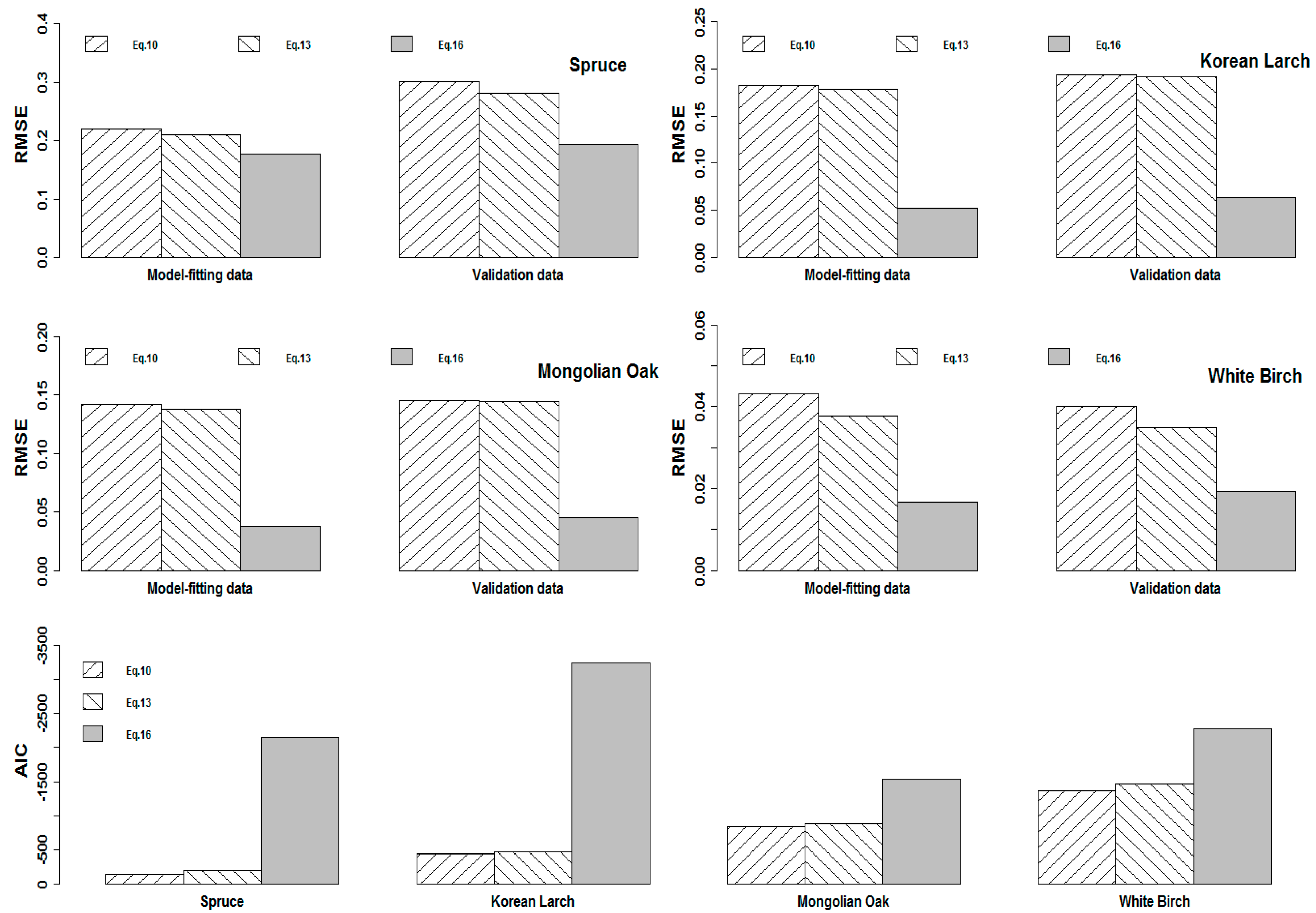
Equations (10), (13), and (16), which had been derived from the base model Equation (3) by isolating parameter, had the most powerful fitting ability for ADA, ADA + DV, and ADA + CM, respectively. The ability of these three equations to make predictions was further compared, based on statistics RMSE and AIC, using both model-fitting and validation data sets, and prediction error statistics for these models are presented in Figure 2.
Figure 2 shows that the prediction accuracy for tree height of Equation (13) was much higher than that of Equation (10). This result indicated that the variability between site type classes could be explained by the site-related fixed-effects parameters in Equation (13). The prediction accuracy of Equation (13) was further improved by considering random effects at sample plot-level on height. For Spruce, Korean Larch, Mongolian Oak, and White Birch, Equation (16) resulted in the decrease of RMSE by 15.45%, 70.52%, 72.59%, and 55.82% for the model-fitting data set, and by 31.34%, 66.72%, 68.40%, and 44.41% for validation data set, compared with Equation (13), respectively. Similarly, the AIC for Spruce, Korean Larch, Mongolian Oak, and White Birch in Equation (16) were 914.25%, 581.69%, 74.08%, and 54.73% smaller than those in Equation (13) for the model-fitting data set, respectively. Such results suggested that the random effects at sample plot level on height variation were substantial and that their inclusion in the model can greatly improve the model’s accuracy of predictions for all stands. Hence, Equation (16) was chosen to predict site productivity for each species when both site-related fixed effects by site type classes and random effects at the sample plot-level were taken into account simultaneously.
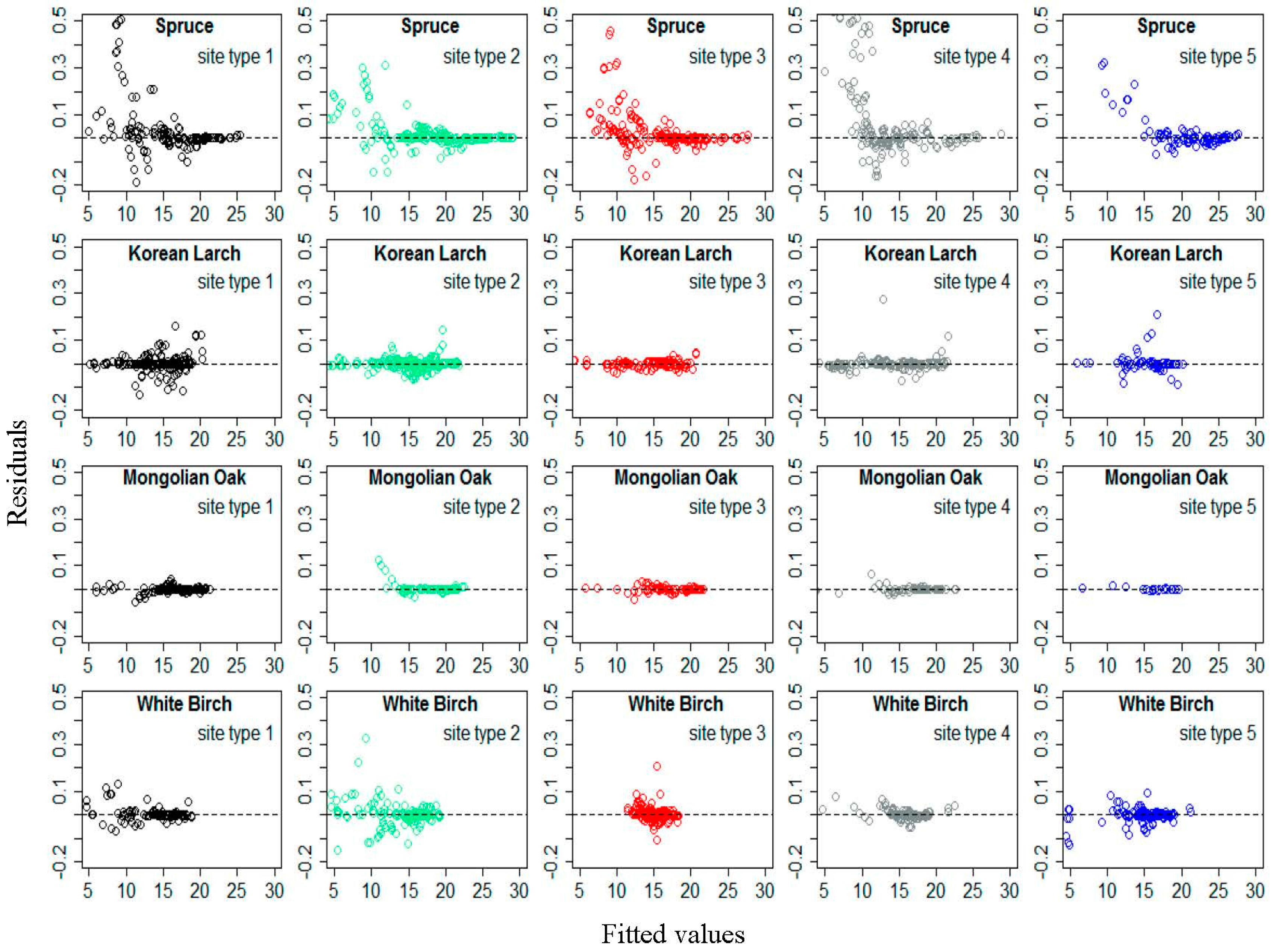
Figure 3 shows residual distributions of Equation (16) for each species by different site type classes, based on the modelling data. The residuals did not show an obvious increasing trend as the predicted height values increased. Similar residual patterns can be found for the validation data as well. This indicated that the exponential variance function applied to D effectively accounted for heteroscedasticity.
3.5. Site Productivity Estimation
If predictors and in Equation (16) were replaced by and , then the model that was used to estimate H from specified and can be expressed as
where and are the dominant height and diameter of the jth sample plot nested in the ith site type, respectively; is an error term. All other variables, parameters, and covariance structures in Equation (22) were already defined in Equation (16). Parameter estimates of Equations (16) and (20) for each species were identical (see Table S8).
The relationships between H and D from Equation (22) under four different classes of for the five site types (Table S1) for each species are shown in Figure 4. The basic form of the D–H curves produced by Equation (22) was a rapid increase in height within stands with low D values; this increase eventually reaches a maximum in stands with high D values, although specific details vary among site types and tree species. All of these curves for each class of SPI passed through the points and for each species. H increased with increases in SPI at constant D for each species. The differences among the relationships between H and D among different classes of SPI at each site type were substantial for each species. This result further verified that Equation (22) produced a polymorphic set of H–D curves with common asymptotes. Figure 4 shows that the differences among the relationships between H and D among different sample plots in the same class of SPI for each species are very large, especially for Korean Larch and Mongolian Oak. This result also indicates that the random variability between sample plots could be accounted for by Equation (22).
4. Discussion
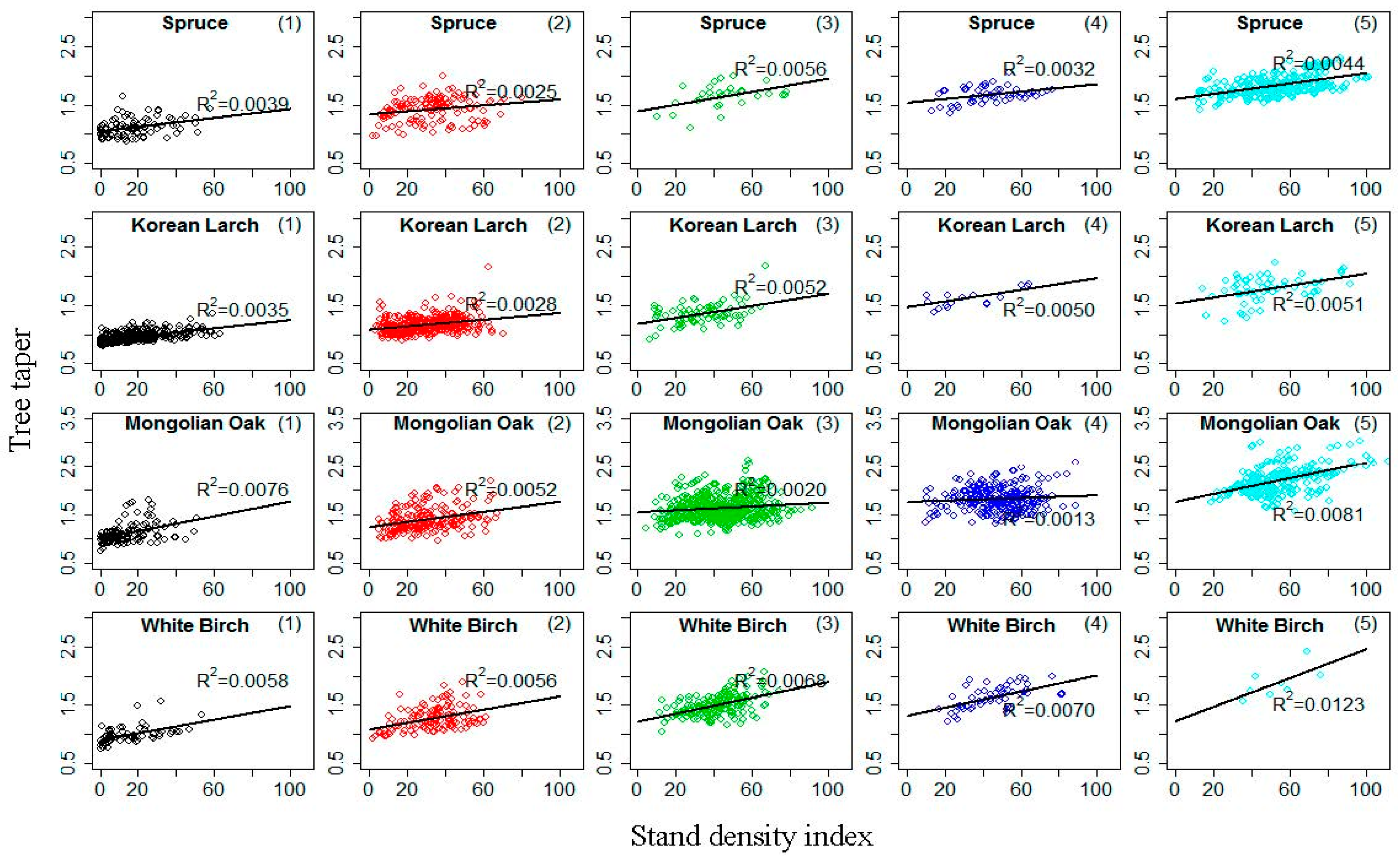
The H–D relationship approach for site productivity estimation was built on three assumptions: (i) decreasing tree taper (D divided by H) is associated with increasing site productivity [7]; (ii) stand density does not affect the H–D relationship of dominant and codominant trees in uneven-aged stands [7]; and (iii) height growth over time is asymptotic, whereas diameter is not. Our study found that the first assumption generally held, with increasing site productivity leading to increasing for a given in Equation (22). This conclusion was verified by Larson’s findings [58], and it has been pointed out that it is unreasonable to test the first assumption by using the relationship of tree taper and SI [26]. The nonsignificant correlation of tree taper and SI could not be used to draw the conclusion that the relationship of tree taper and site productivity is not significant for natural forests, especially when site productivity is estimated by the H–D relationship method. Stout and Shumway [23] discussed the second assumption in detail and concluded that the influence of stand density on potential site productivity assessment using the H–D relationship was minimal. Increasing stand density has been found to reduce both H and D growth for mixed stands, also implying that the stand density impact on the H–D relationship will probably be minimized, especially if this relationship is only considered for the dominant and codominant trees in the stands [7]. A stand density index ( is the number of trees per hectare, is average diameter of trees, is the standard base diameter (26.4 cm, 23.8 cm, 23.7 cm and 21.2 cm for Spruce, Korean Larch, Mongolian Oak, and White Birch in this study, respectively), and parameter ) that is often used to describe stand density information in forestry [59] was applied to test the second assumption. Figure 5 provides scatterplots of tree taper against within five age classes for the four natural uneven-aged pure stands, with lines illustrating a linear relationship between the two variables. The plots indicate that tree taper is not significantly correlated with for the four stands. This result suggests that the effect of stand density on the H–D relationship was minimal, especially if this relationship was only considered for dominant and codominant trees in stands. For the third assumption, Equation (22) produced an anamorphic set of H–D curves with site type-related asymptotes (Figure 4); however, there was no limitation for diameter based on the model. Similar to the conclusion obtained by Huang and Titus [7], although the use of SPI as determined by the dominant and codominant H–D relationship is by no means the final solution, it provides a simple and reasonable index of site productivity for the four main natural uneven-aged pure stands of Spruce, Korean Larch, Mongolian Oak, and White Birch in northeastern China (Figure 4).
The dominant height in the traditional ADA was estimated from the last time measurements of , and the current by Equations (9)–(11). However, from a statistical point of view, the H–D curves obtained from Equations (9)–(11) are inconsistent with height prediction, as ADA was a population average (PA) approach [60]. The PA approach does not recognize SS variability in height curves in the fitting stage. In contrast, Equations (12)–(14), developed through ADA + DV based on Equations (9)–(11), could be used to relate site type to SS prediction, by assigning the asymptote parameters in Equations (12)–(14) as site type–specific (local), while the other parameters are global (common). In addition to recognizing SS variability in the height curves, Equations (12)–(14) also had much higher fitting accuracy than Equations (9)–(11) (see Tables S5 and S7). This is mainly because Equations (12)–(14) successfully explained the differences in the effects of site type classes on H. In practice, many sample plots used for developing H–D curves are selected randomly. In this study, although Equation (17) did not converge on some data in the fitting, Equations (15) and (16), developed through ADA + CM based on Equations (12) and (13), could be used to account for the random effects on the H–D relationship at sample plot level (Table S8). Fitting accuracy of the converged Equations (15) and (16), developed through ADA + CM, was much higher than that of Equations (12) and (13), developed through ADA + DV. Our results further supported the conclusions of Calama and Montero [30] and Adame et al. [44] that the random effects of sample plots on the H–D relationship are significant and cannot be neglected in modelling.
Equations (15) and (16) could be applied to predict H, with or without assuming random effects. The model without random effects was known as a mean response (M response), while the model with random effects was known as an SS or localized model. The localization process is also referred to as model calibration [36]. The predictions of the M response model did not require prior information for a response variable; that is, dominant height measured from a sub-sample of the trees is not needed. However, such dominant height measurement is required if the model has random effects. Many previous studies [30,31,32,33,34,35,36,37,38,39,40,41,42,43,44] applied the two models to predict height in developing the H–D relationship using the NLME approach and concluded that the prediction accuracy of the SS model was much higher than that of the M response. In this study, only the SS model was used for H prediction in Equations (15) and (16). When the M response method was applied for H prediction in Equations (15) and (16), the prediction accuracy was much lower than that of the SS method, which corroborates the findings in the studies by Calama and Montero [30] and Adame et al. [44]. For example, for White Birch, the values of , and from Equation (16) (SS method) were 65.38%, 59.11%, and 83.28% smaller than those from the M response method for the model-fitting data set, and 86.35%, 47.51% and 57.29% smaller than the M response method for the validation data set, respectively.
An implicit assumption shared by ADA, ADA + DV, and ADA + CM approaches is that independent variables (, and ) in the models developed through these methods are measured without errors. This assumption may be valid for and , which can be easily and accurately measured in the field. However, this assumption cannot apply to , because this variable is often difficult to measure. This is especially true in natural uneven-aged stands [61]. It is well known that the violation of this assumption may lead to biased estimates of regression coefficients as well as their standard errors and thus to invalid statistical inferences [62]. The biased estimates of parameters will definitely reduce the prediction accuracy of site productivity. If predictor variables in Equations (9)–(17) are considered to have measurement errors, a new NLME approach needs to be developed. However, no algorithm and corresponding computational program to implement this approach is available to date, and we are in the process of developing such algorithm to solve this problem.
The proposed ADA + DV and ADA + CM approaches are relatively more complicated and difficult to implement than the traditional ADA approach. However, the prediction accuracies of both ADA + DV and ADA + CM approaches are much higher than that of traditional ADA approach (Figure 2). In practical application, if we just focus on the practicability of the H–D models and do not recognize the site type or sample plot specific variability in site productivity estimation, the traditional ADA approach is strongly recommended. Otherwise, the proposed ADA + DV or ADA + CM approaches are recommended to make SS predictions to guarantee a high accuracy of the estimates of site productivity. In this study, both site-related fixed effects by site type classes and random effects at the sample plot-level on site productivity were substantial, therefore, Equation (22) was applied to estimate the site productivity in natural uneven-aged pure stands in northeastern China. The variability between site type classes and between sample plots could be effectively explained by Equation (22) simultaneously (Figure 4). It should be noted that recalibration of SPI cures with PSP data source is thus particularly important for long-lived and shade-tolerant species that seem to have active tree replacement dynamics in the dominant stratum [47].
The focus of this study was mainly on methodological development. The applicability of the developed H–D models would be influenced by other environmental variables, such as climate variables. Most of the recently published studies on forest productivity have demonstrated high possibility of incorporating the changes in site conditions [63,64,65,66,67,68,69,70,71]. In this study, climate variables need to be incorporated into dominant H–D models if these models are utilized to directly account for the impact of changing climate on forest site productivity. This can be easily accomplished, at least, in the composite model form, by modifying the intercept term (i.e., ) in H–D models such as Models (1)–(3). Bontemps and Bouriaud [69] formulated perspectives regarding the increase of prediction accuracy of forest productivity by introducing environmental indicators and including information on genetic structure of tree populations in the context of adaptation to future climate change, as well as the use of site productivity models in forest management. Fu et al. [72] developed a game-theoretic related H–D model and found that the effect of genetic architecture on H–D relationship was substantial. Based on these studies, we are in the process of developing climate- and genetic-related H–D models using the proposed method to estimate the forest site productivity for natural uneven-aged stands in northeastern China.
5. Conclusions
In this study, we developed dominant H–D models to estimate forest site productivity using traditional ADA, ADA + DV, and ADA + CM approaches for four main natural uneven-aged pure stands in northeastern China. We found that the models developed by ADA, ADA + DV, and ADA + CM had high fitting accuracy overall. Among these methods, the models developed from ADA + CM displayed the best performance, followed by the models from ADA+DV, and the models developed from ADA performed the worst. The results show that the random effects at sample plot level on the variation of the height and diameter relationship were substantial and that their inclusion in the model greatly improved its accuracy of predictions for each natural uneven-aged pure stand. The results of this study also indicated that the dominant H–D relationship based on SPI provided an effective method for quantifying site type- and sample plot-specific site productivity for uneven-aged pure stands in northeastern China, which corroborated the findings from previous studies [7,18]. Furthermore, this method used for estimating site productivity required no time-consuming and difficult age measurements, but only H and D measurements, which were readily obtainable from ordinary inventories and compatible with the existing national forest inventory data-collection process in China.
Supplementary Materials
The following are available online at https://www.mdpi.com/1999-4907/9/2/63/s1, Table S1: Permanent sample plots and observations of each natural uneven-aged pure stand (Spruce, Korean Larch, Mongolian Oak, and White Birch) within five site types (see Table 1); Table S2: Summary statistics for model-fitting and validation data sets. Min, minimum; Max, maximum; SD, standard deviation; D, diameter at breast height of dominant tree; and H, total height of dominant tree; Table S3: Root mean square error for candidate base Equations (1)–(3); Table S4 Parameter estimates of Equations (9)–(11). , fixed-effects parameters; and , variance-covariance parameter of error term; Table S5 Evaluation indexes of Equations (9)–(11) for algebraic difference approach. , root mean square error; and AIC, Akaike’s information criterion; Table S6 Parameter estimates of Eqs. 12-14. , , , , and = fixed-effects parameters; and for Equation (12), and for Equation (13), and for Equation (14); and , parameters of variance-covariance for error term; Table S7 Evaluation indexes of Equations (12)–(14). , root mean square error; and AIC, Akaike’s information criterion; Table S8 Parameter estimates of Equations (15) and (16). , , , , and = fixed-effects parameters; and for Equation (15), and for Equation (16); , parameter of variance-covariance for random effects; and , and , parameters of variance-covariance for error term; and Table S9 Evaluation indexes of Eqs. 15 and 16. , root mean square error; and AIC, Akaike’s information criterion.
Acknowledgments
We thank the Forestry Public Welfare Scientific Research Project (No. 201504303)and the Chinese National Natural Science Foundations (Nos. 31470641, 31300534, and 31570628) for the financial support of this study. We are grateful to Shouzheng Tang, Xiangdong, Lei, Haikui Li, lingxia Hong, Yuancai Lei, Hong Guo, and other researchers in the Chinese Academy of Forestry for their valuable suggestions on this study.We also appreciate the valuable comments and the constructive suggestions from two anonymous referees and the associate Editor that helped improved the manuscript.
Author Contributions
L.F. and G.D. conceived the idea and designed methodology; L.F. and Q.W. collected data; L.F. and Z.G. analyzed data; and L.F. and G.D. wrote the manuscript and contributed critically to improve the manuscript, and gave a final approval for publication.
Conflicts of Interest
The authors declare no competing financial interests.
References
- Berrill, J.; O’Hara, K. Estimating site productivity in irregular stand structures by indexing the basal area or volume increment of the dominant species. Can. J. For. Res. 2014, 44, 92–100. [Google Scholar] [CrossRef]
- Carmean, W.H. Forest site quality evaluation in the United States. Adv. Agron. 1975, 27, 209–267. [Google Scholar]
- Alemdag, I.S. National site-index and height-growth curves for white spruce growing in natural stands in Canada. Can. J. For. Res. 1991, 21, 1466–1474. [Google Scholar] [CrossRef]
- Szwaluk, K.S.; Strong, W.L. Near-surface soil characteristics and understory plants as predictors of Pinus contorta site index in Southwestern Alberta, Canada. For. Ecol. Manag. 2003, 176, 13–24. [Google Scholar] [CrossRef]
- Devan, J.S.; Burkhart, H.E. Polymorphic site index equation for loblolly pine based on a segmented polynomial differential model. For. Sci. 1982, 28, 544–555. [Google Scholar]
- Biging, G.S. Improved estimates of site index curves using a varying-parameter model. For. Sci. 1985, 31, 248–259. [Google Scholar]
- Huang, S.; Titus, S.J. An index of site productivity for uneven-aged or mixed-species stands. Can. J. For. Res. 1993, 23, 558–562. [Google Scholar] [CrossRef]
- Corona, P.; Scotti, R.; Tarchiani, N. Relationship between environmental factors and site index in Douglas-fir plantations in central Italy. For. Ecol. Manag. 1998, 110, 195–207. [Google Scholar] [CrossRef]
- McKenney, D.W.; Pedlar, J.H. Spatial models of site index based on climate and soil properties for two boreal tree species in Ontario, Canada. For. Ecol. Manag. 2003, 175, 497–507. [Google Scholar] [CrossRef]
- Bergès, L.; Chevalier, R.; Dumas, Y.; Franc, A.; Gilbert, J.M. Sessile oak (Quercus petraea Liebl.) site index variations in relation to climate, topography and soil in even-aged high-forest stands in northern France. Ann. For. Sci. 2005, 62, 391–402. [Google Scholar] [CrossRef]
- Aertsen, W.; Kint, V.; Van Orshoven, J.; Özkan, K.; Muys, B. Comparison and ranking of different modelling techniques for prediction of site index in Mediterranean mountain forests. Ecol. Model. 2010, 221, 1119–1130. [Google Scholar] [CrossRef]
- Aertsen, W.; Kint, V.; Orshoven, J.V.; Muys, B. Evaluation of modelling techniques for forest site productivity prediction in contrasting ecoregions using stochastic multicriteria acceptability analysis (SMAA). Environ. Model. Softw. 2011, 26, 929–937. [Google Scholar] [CrossRef] [Green Version]
- Jiang, H.; Radtke, P.J.; Weiskittel, A.R.; Coulston, J.W.; Guertin, P.J. Climate- and soil-based models of site productivity in eastern US tree species. Can. J. For. Res. 2015, 45, 325–342. [Google Scholar] [CrossRef]
- Diaci, J.; Kerr, G.; O’Hara, K. Twenty-first century forestry: Integrating ecologically based, uneven-aged silviculture with increased demands on forests. Forestry 2011, 84, 463–465. [Google Scholar] [CrossRef]
- Carmean, W.H.; Lenthall, D.J. Height growth and site index curve for jack pine in north central Ontario. Can. J. For. Res. 1989, 19, 215–224. [Google Scholar] [CrossRef]
- Trasobares, A.; Pukkalab, T. Using past growth to improve individualtree diameter growth models for uneven-aged mixtures of Pinus sylvestris L. and Pinus nigra Arn. in Catalonia, north-east Spain. Ann. For. Sci. 2004, 61, 409–417. [Google Scholar] [CrossRef]
- Palahí, M.; Pukkala, T.; Kasimiadis, D.; Poirazidis, K.; Papageorgiou, A.C. Modelling site quality and individual-tree growth in pure and mixed Pinus brutia stands in north-east Greece. Ann. For. Sci. 2008, 65, 1–24. [Google Scholar] [CrossRef]
- Vanclay, J.K.; Henry, N.B. Assessing site productivity of indigenous cypress pine forest in southern Queensland. Commonw. For. Rev. 1988, 67, 53–64. [Google Scholar]
- Trorey, L.G. A mathematical method for the construction of diameter-height curves based on site. For. Chron. 1932, 8, 121–132. [Google Scholar] [CrossRef]
- Meyer, H.A. A mathematical expression for height curves. J. For. 1940, 38, 415–420. [Google Scholar]
- Husch, B.; Miller, C.I.; Beers, T.W. Forest Mensuration, 3rd ed.; John Wiley and Sons: New York, NY, USA, 1982. [Google Scholar]
- McLintock, T.F.; Bickford, C.A. A Proposed Site Index for Red Spruce in the Northeast; Paper 93; U.S. Department of Agriculture, Forest Service, Northeastern Forest Experiment Station: Upper Darby, PA, USA, 1957.
- Stout, B.B.; Shumway, D.L. Site quality estimation using height and diameter. For. Sci. 1982, 28, 639–645. [Google Scholar]
- Herrera-Fernández, J.J.; Campos, J.J.; Kleinn, C. Site productivity estimation using height-diameter relationships in Costa Rican secondary forests. Investig. Agrar. Sist. Recur. For. 2004, 13, 295–303. [Google Scholar]
- Fu, L.; Lei, X.; Li, H.; Hong, L.; Zhu, G.; Guo, H.; Tang, S. Site quality evaluation of natural forest based on height-diameter model. Sci. Silv. Sin. in press.
- Wang, G.G. Is height of dominant trees at a reference diameter an adequate measure of site quality? For. Ecol. Manag. 1998, 112, 49–54. [Google Scholar] [CrossRef]
- Curtis, R.O. Height-diameter and height-diameter-age equations for second-growth Douglas-fir. For. Sci. 1967, 13, 365–375. [Google Scholar]
- Pokharel, B.; Froese, R.E. Representing site productivity in the basal area increment model for FVS-Ontario. For. Ecol. Manag. 2009, 258, 657–666. [Google Scholar] [CrossRef]
- Hall, D.B.; Clutter, M. Multivariate multilevel nonlinear mixed effects models for timber yield predictions. Biometrics 2004, 60, 16–24. [Google Scholar] [CrossRef] [PubMed]
- Calama, R.; Montero, G. Interregional nonlinear height-diameter model with random coefficients for stone pine in Spain. Can. J. For. Res. 2004, 34, 150–163. [Google Scholar] [CrossRef]
- Schabenberger, O.; Gregoire, T.G. A conspectus on estimating function theory and its application to recurrent modelling issues in forest biometry. Silv. Fenn. 1995, 29, 49–70. [Google Scholar]
- West, P.W.; Ratkowsky, D.A.; Davis, A.W. Problems of hypothesis testing of regressions with multiple measurements from individual sampling units. For. Ecol. Manag. 1984, 7, 207–224. [Google Scholar] [CrossRef]
- Gregoire, T.G.; Schabenberger, O.; Barrett, J.P. Linear modeling of irregularly spaced, unbalanced, longitudinal data from permanent plot measurements. Can. J. For. Res. 1995, 25, 137–156. [Google Scholar] [CrossRef]
- Hall, D.B.; Bailey, R.L. Modeling and prediction of forest growth variables based on multilevel nonlinear mixed models. For. Sci. 2001, 47, 311–321. [Google Scholar]
- Nanos, N.; Rafael, C.; Gregorio, M.; Luis, G. Geostatistical prediction of height-diameter models. For. Ecol. Manag. 2004, 195, 221–235. [Google Scholar] [CrossRef]
- Meng, S.X.; Huang, S. Improved calibration of nonlinear mixed-effects models demonstrated on a height growth function. For. Sci. 2009, 55, 239–248. [Google Scholar]
- Yang, Y.; Huang, S. Comparison of different methods for fitting nonlinear mixed forest models and for making predictions. Can. J. For. Res. 2011, 41, 1671–1686. [Google Scholar] [CrossRef]
- Rijal, B.; Weiskittel, A.R.; Kershaw, J.A. Development of height to crown base models for thirteen tree species of the North American Acadian Region. For. Chron. 2012, 88, 60–73. [Google Scholar] [CrossRef]
- Fu, L.; Sun, H.; Sharma, R.P.; Lei, Y.; Zhang, H.; Tang, S. Nonlinear mixed-effects crown width models for individual trees of Chinese fir (Cunninghamia lanceolata) in south-central China. For. Ecol. Manag. 2013, 302, 210–220. [Google Scholar] [CrossRef]
- Sharma, R.P.; Breidenbach, J. Modeling height-diameter relationships for Norway spruce, Scots pine, and downy birch using Norwegian national forest inventory data. For. Sci. Technol. 2015, 11, 44–53. [Google Scholar] [CrossRef]
- Sharma, R.P.; Vacek, Z.; Vacek, S. Individual tree crown width models for Norway spruce and European beech in Czech Republic. For. Ecol. Manag. 2016, 366, 208–220. [Google Scholar] [CrossRef]
- Lindstrom, M.J.; Bates, D.M. Nonlinear mixed effects models for repeated measures data. Biometrics 1990, 46, 673–687. [Google Scholar] [CrossRef] [PubMed]
- Vonesh, E.F.; Chinchilli, V.M. Linear and Nonlinear Models for the Analysis of Repeated Measurements; Marcel Dekker: New York, NY, USA, 1997. [Google Scholar]
- Adame, P.; Río, M.D.; Cañellas, I. A mixed nonlinear height diameter model for Pyrenean oak (Quercus pyrenaica Willd.). For. Ecol. Manag. 2008, 256, 88–98. [Google Scholar] [CrossRef]
- Crecente-Campo, F.; Tomé, M.; Soares, P.; Dieguez-Aranda, U. A generalized nonlinear mixed-effects height-diameter model for Eucalyptus globulus L. in northwestern Spain. For. Ecol. Manag. 2010, 259, 943–952. [Google Scholar] [CrossRef]
- Zhang, W.R.; Jiang, Y.X. The Forest Site of China; Science Press: Beijing, China, 1997; pp. 1–32. (In Chinese) [Google Scholar]
- Raulier, F.; Lambert, M.; Pothier, D.; Ung, C. Impact of dominant tree dynamics on site index curves. For. Ecol. Manag. 2003, 184, 65–78. [Google Scholar] [CrossRef]
- Rozas, V. Tree age estimates in Fagus sylvatica and Quercus robur: Testing previous and improved methods. Plant Ecol. 2003, 167, 193–212. [Google Scholar] [CrossRef]
- Venables, W.N.; Ripley, B.D. Modern Applied Statistics with S-PLUS, 3rd ed.; Springer: New York, NY, USA, 1999. [Google Scholar]
- Huuskonen, S.; Miina, J. Stand-level growth models for young scots pine stands in Finland. For. Ecol. Manag. 2007, 241, 49–61. [Google Scholar] [CrossRef]
- Bailey, R.L.; Clutter, J.L. Base-age invariant polymorphic site curves. For. Sci. 1974, 20, 155–159. [Google Scholar]
- Uis, F.; Margarida, T.; Marta, B.C. Modelling dominant height growth of Douglas-fir (Pseudotsuga menziesii (Mirb.) Franco) in Portugal. Forestry 2003, 76, 509–523. [Google Scholar]
- Cieszewski, C.J.; Strub, M.R. Generalized algebraic difference approach derivation of dynamic site equations with polymorphism and variable asymptotes from exponential and logarithmic functions. For. Sci. 2008, 54, 303–315. [Google Scholar]
- Wang, M.; Borders, B.E.; Zhao, D. An empirical comparison of two subject-specific approaches to dominant heights modeling: The dummy variable method and the mixed model method. For. Ecol. Manag. 2008, 255, 2659–2669. [Google Scholar] [CrossRef]
- Tang, S.Z.; Li, Y.; Fu, L.Y. Statistical Foundation for Biomathematical Models, 2nd ed.; Higher Education Press: Beijing, China, 2015; 435p. (In Chinese) [Google Scholar]
- Davidian, M.; Giltinan, D.M. Nonlinear Models for Repeated Measurement Data; Chapman and Hall: New York, NY, USA, 1995. [Google Scholar]
- Pinheiro, J.C.; Bates, D.M. Mixed-Effects Models in S and S-PLUS; Spring: New York, NY, USA, 2000. [Google Scholar]
- Larson, P.R. Stem form development of forest trees. For. Sci. Monogr. 1963, 9, 31. [Google Scholar] [CrossRef]
- Tang, S.; Meng, C.H.; Meng, F.; Wang, Y.H. A growth and self-thinning model for pure even-age stands: Theory and applications. For. Ecol. Manag. 1994, 70, 67–73. [Google Scholar] [CrossRef]
- Zeger, S.L.; Liang, K.; Albert, P.S. Models for longitudinal data: A generalized estimating equation approach. Biometrics 1988, 44, 1049–1060. [Google Scholar] [CrossRef] [PubMed]
- Marshall, H.D.; Murphy, G.E.; Boston, K. Evaluation of the economic impacts of length and diameter measurement error on mechanical harvesters and processors operating in pine stands. Can. J. For. Res. 2006, 36, 1661–1673. [Google Scholar] [CrossRef]
- Fuller, W.A. Measurement Error Models; John Wiley and Sons: New York, NY, USA, 1987. [Google Scholar]
- Bontemps, J.-D.; Hervé, J.-C.; Dhǒte, J.-F. Long-term changes in orest productivity: A consistent assessment in even-aged stands. For. Sci. 2014, 55, 549–564. [Google Scholar]
- Coops, N.C.; Coggins, S.B.; Kurz, W. Mapping the environmental limitations to growth of coastal Douglas-fir stands on Vancouver Island, British Columbia. Tree Physiol. 2007, 27, 805–815. [Google Scholar] [CrossRef] [PubMed]
- Coops, N.C.; Hember, R.; Waring, R.H. Assessing the impact of current and projected climates on Douglas-fir productivity in British Columbia, Canada, using a process-based model (3-PG). Can. J. For. Res. 2010, 40, 511–524. [Google Scholar] [CrossRef]
- Skovsgaard, J.P.; Vanclay, J.K. Forest site productivity: A review of the evolution of dendrometric concepts for even-aged stands. Forestry 2008, 81, 13–31. [Google Scholar] [CrossRef]
- Nothdurft, A.; Wolf, T.; Ringeler, A.; Böhner, J.; Saborowski, J. Spatio-temporal prediction of site index based on forest inventories and climate change scenarios. For. Ecol. Manag. 2012, 279, 97–111. [Google Scholar] [CrossRef]
- Skovsgaard, J.P.; Vanclay, J.K. Forest site productivity: A review of spatial and temporal variability in natural site conditions. Forestry 2013, 86, 305–315. [Google Scholar] [CrossRef]
- Bontemps, J.-D.; Bouriaud, O. Predictive approaches to forest site productivity: Recent trends, challenges and future perspectives. Forestry 2014, 87, 109–128. [Google Scholar] [CrossRef]
- Socha, J.; Coops, N.C.; Ochal, W. Assessment of age bias in site index equations. iForest 2016, 9, e1–e7. [Google Scholar] [CrossRef]
- Charru, M.; Seynave, I.; Hervé, J.-C.; Bertrand, R.; Bontemps, J.-D. Recent growth changes in Western European forests are driven by climate warming and structured across tree species climatic habitats. Ann. For. Sci. 2017, 74, 33. [Google Scholar] [CrossRef]
- Fu, L.; Jiang, L.; Ye, M.; Sun, L.; Tang, S.; Wu, R. How trees allocate stem carbon for optimal growth: Insight from a game-theoretic model. Brief. Bioinform. 2017. [Google Scholar] [CrossRef] [PubMed]
Figure 1.
Permanent sample plots (PSPs) of four main natural uneven-aged pure stands (95, 72, 105, and 77 PSPs for Spruce, Korean Larch, Mongolian Oak, and White Birch, respectively, for a total of 349) distributed over almost the entire middle and eastern area of Jilin province. Figure was created using Esri ArcGIS 9.3 (http://www.esri.com/software/arcgis/arcgis-for-desktop).
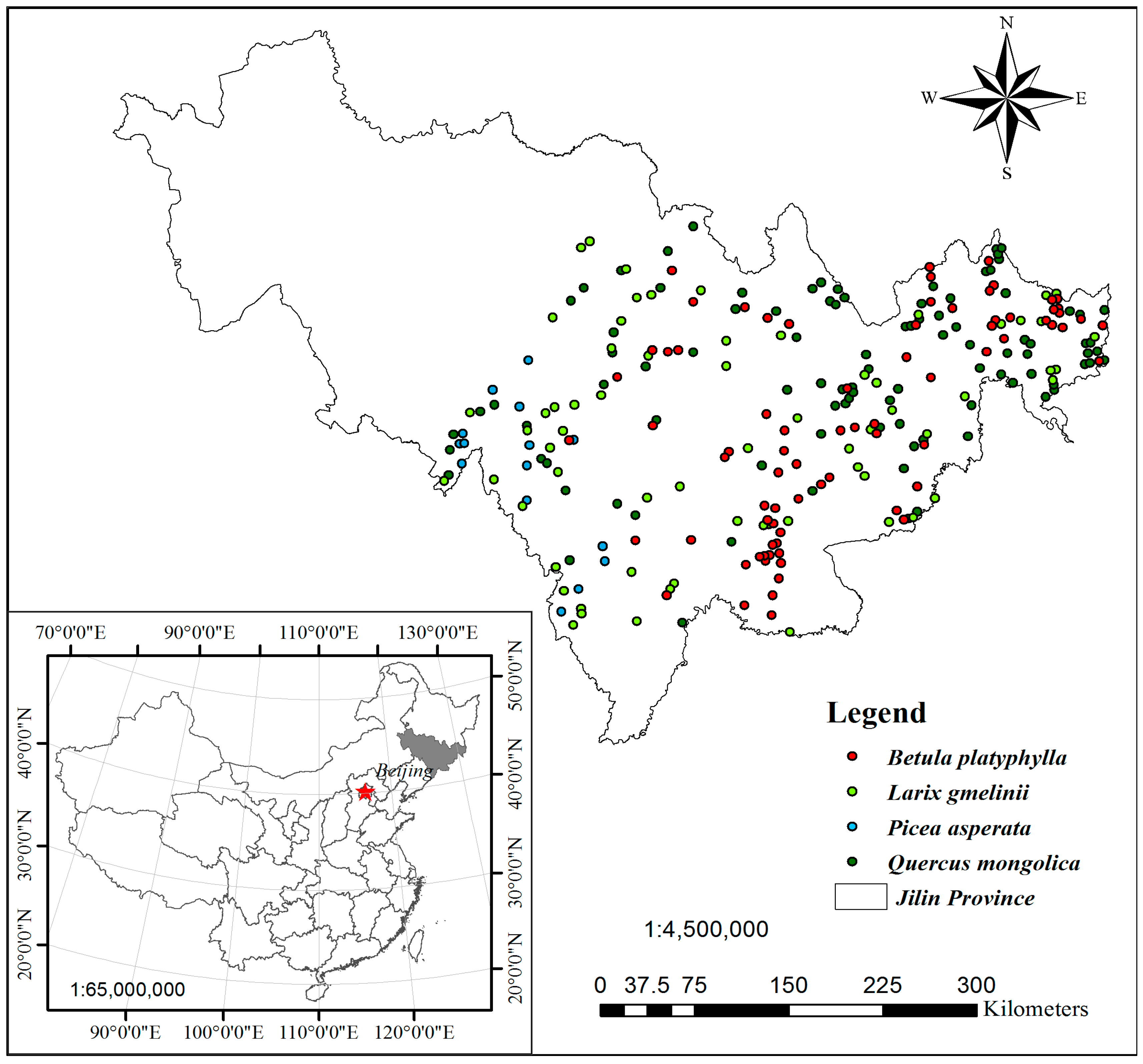
Figure 2.
Comparisons of performance among Equations (10), (13), and (16) for Spruce, Korean Larch, Mongolian Oak, and White Birch based on root mean square error (RMSE) and Akaike’s information criterion (AIC) using both model-fitting and validation data sets.
Figure 2.
Comparisons of performance among Equations (10), (13), and (16) for Spruce, Korean Larch, Mongolian Oak, and White Birch based on root mean square error (RMSE) and Akaike’s information criterion (AIC) using both model-fitting and validation data sets.

Figure 3.
Residual distribution of Equation (16) for Spruce, Korean Larch, Mongolian Oak, and White Birch according to different site type classes.
Figure 3.
Residual distribution of Equation (16) for Spruce, Korean Larch, Mongolian Oak, and White Birch according to different site type classes.

Figure 4.
The relationships between dominant height (H) and dominant diameter (D) from Equation (22) under four classes of site productivity index (SPI) (12 m, 14 m, 16 m, and 18 m for Spruce, Mongolian Oak, and White Birch, and 14 m, 17 m, 20 m, and 23 m for Korean Larch) according to five different site types (1–5, Table 1) for four natural uneven-aged pure stands of Spruce, Korean Larch, Mongolian Oak, and White Birch; dotted line denotes the dominant heights at the base diameter.
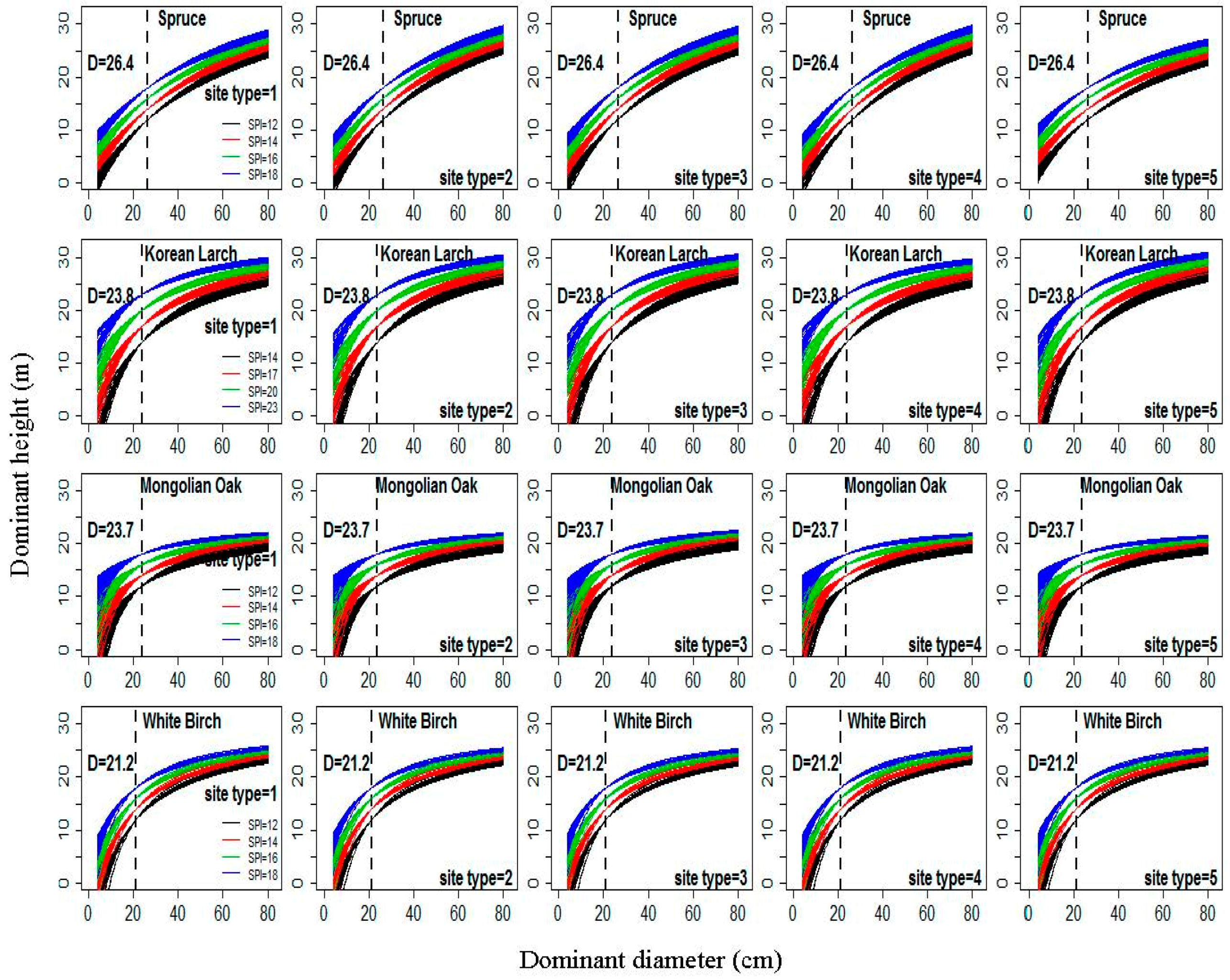
Figure 5.
Scatterplot of tree taper against stand density index within five age classes (all dominant and codominant trees were stratified into the first four age classes [1,2,3,4,5] based on age intervals of 20 years; the fifth class was age >80 years) for four natural uneven-aged pure stands of Spruce, Korean Larch, Mongolian Oak, and White Birch; lines illustrate linear relationship between the two variables.


Table 1.
Five main site types for permanent sample plots in Jilin province.
| Number | Temperature | Humidity | Topography | Soil Depth | Soil Type |
|---|---|---|---|---|---|
| 1 | Mid-temperature | Sub-humid | Low mountain rolling hills, gentle southeast slope, downslope | Medium | Dark brown |
| 2 | Mid-temperature | Sub-humid | Low mountain rolling hills, gentle southeast slope, middle slope | Medium | Dark brown |
| 3 | Mid-temperature | Sub-humid | Low mountain rolling hills, gentle northeast slope, middle slope | Medium | Dark brown |
| 4 | Mid-temperature | Humid | Low mountain rolling hills, gentle southeast slope, upslope | Medium | Dark brown |
| 5 | Mid-temperature | Humid | Low mountain rolling hills, gentle northeast slope, upslope | Medium | Dark brown |
© 2018 by the authors. Licensee MDPI, Basel, Switzerland. This article is an open access article distributed under the terms and conditions of the Creative Commons Attribution (CC BY) license (http://creativecommons.org/licenses/by/4.0/).
Share and Cite
MDPI and ACS Style
Duan, G.; Gao, Z.; Wang, Q.; Fu, L. Comparison of Different Height–Diameter Modelling Techniques for Prediction of Site Productivity in Natural Uneven-Aged Pure Stands. Forests 2018, 9, 63. https://doi.org/10.3390/f9020063
AMA Style
Duan G, Gao Z, Wang Q, Fu L. Comparison of Different Height–Diameter Modelling Techniques for Prediction of Site Productivity in Natural Uneven-Aged Pure Stands. Forests. 2018; 9(2):63. https://doi.org/10.3390/f9020063
Chicago/Turabian StyleDuan, Guangshuang, Zhigang Gao, Qiuyan Wang, and Liyong Fu. 2018. "Comparison of Different Height–Diameter Modelling Techniques for Prediction of Site Productivity in Natural Uneven-Aged Pure Stands" Forests 9, no. 2: 63. https://doi.org/10.3390/f9020063
Note that from the first issue of 2016, this journal uses article numbers instead of page numbers. See further details here.