The Impact of Green Space Layouts on Microclimate and Air Quality in Residential Districts of Nanjing, China


1
School of Architecture and Urban Planning, Nanjing University, 22 Hankou Road, Nanjing 210093, China
2
Dipartimento di Scienze e Tecnologie Biologiche ed Ambientali, University of Salento, S.P. 6 Lecce-Monteroni, 73100 Lecce, Italy
*
Author to whom correspondence should be addressed.
Forests 2018, 9(4), 224; https://doi.org/10.3390/f9040224
Submission received: 6 February 2018
/
Revised: 31 March 2018
/
Accepted: 16 April 2018
/
Published: 23 April 2018
(This article belongs to the Special Issue Advances in Modelling Vegetation and Forests in the Urban Environment: Local Climate and Air Quality)
Abstract
:This study numerically investigates the influence of different vegetation types and layouts on microclimate and air quality in residential districts based on the morphology and green layout of Nanjing, China. Simulations were performed using Computational Fluid Dynamics and the microclimate model ENVI-met. Four green indices, i.e., the green cover ratio, the grass and shrub cover ratio, the ecological landscaping plot ratio and the landscaping isolation index, were combined to evaluate thermal and wind fields, as well as air quality in district models. Results show that under the same green cover ratio (i.e., the same quantity of all types of vegetation), the reduction of grass and shrub cover ratio (i.e., the quantity of grass and shrubs), replaced by trees, has an impact, even though small, on thermal comfort, wind speed and air pollution, and increases the leisure space for occupants. When trees are present, a low ecological landscaping plot ratio (which expresses the weight of carbon dioxide absorption and is larger in the presence of trees) is preferable due to a lower blocking effect on wind and pollutant dispersion. In conjunction with a low landscaping plot ratio, a high landscaping isolation index (which means a distributed structure of vegetation) enhances the capability of local cooling and the general thermal comfort, decreasing the average temperature up to about 0.5 °C and the average predicted mean vote (PMV) up to about 20% compared with the non-green scenario. This paper shows that the relationship vegetation-microclimate-air quality should be analyzed taking into account not only the total area covered by vegetation but also its layout and degree of aggregation.
1. Introduction
Thermal comfort and air quality are major concerns for people living in urban areas. Currently, due to the influence of factors such as building density, building materials and anthropogenic heat emission in residential areas, high temperatures may frequently occur in hot summers and may negatively affect residential life. Moreover, traffic-induced emissions are one of the major contributors of air pollution in urban built-up areas, emitting several harmful pollutants in the form of particulate matters, such as PM10 [1], PM2.5 [2] and Ultrafine Particles (UFP) [3,4], and gaseous pollutants such as nitrogen oxides (NOx) [5,6] and carbon monoxide (CO) [7].
In the built environment, temperature are generally higher than in the surrounding rural areas, as a result of the low short-wave albedo of city surface, the high heat capacity of building materials, the blockage of outgoing long-wave radiation and natural ventilation by the urban geometry as well as low evaporation rates. Outdoor spaces in the residential area are places for citizens to participate in social activities, so the comfort and air quality directly influence the livability of a residential district. Green space plays an important role in this sense, as well as in its botanical, aesthetic or environmental value [8,9]. Residential green space provides residents with rest and recreational functions of living land by using green infrastructure. Chinese domestic standards (GBJ137-90, CJJ/T85-2002) recommend that urban residential land should account for about 20–30% of the total urban land area, and green space should at least account for 30% in new residential districts. Generally, green spaces in residential areas can be divided into the following four categories: public green spaces, private green spaces, green spaces between buildings and roadside green spaces. Apart from the aesthetic value, vegetation has positive effects on reducing local temperature through shading and evapotranspiration [10,11] and wind flow blocking, especially on cold windy days. In addition, many studies have shown that vegetation can remove pollutants more efficiently from the atmosphere than artificial surfaces because vegetation foliage can absorb gaseous pollutants through their stomata and can remove deposited particles [12,13,14]. Actually, the effect of vegetation on air quality is regarded as a paradox as the aerodynamic and deposition effects of vegetation counterbalance each other. The deposition of particles on vegetation surfaces can be influenced by various factors, such as the diameter and shape of the particles, the planting configuration and meteorological parameters. Although the deposition on vegetation helps to remove particles from the air [15,16,17,18], the aerodynamic effects may reduce the air exchange compared with a no-green scenario, reducing mixing, dilution and ventilation [18,19,20,21,22].
Given the growing interest in outdoor thermal comfort and the well-being of urban residents, a number of models have been developed to investigate the micro-scale outdoor environment, for example, CTTC [23], SOLWEIG [24], RayMan [25], ENVI-met [26]. ENVI-met 4.3 was selected here because of its capacity to simulate the influence of vegetation by combining the simulation of processes induced by vegetation with atmospheric processes occurring in the upper atmospheric layer of built environments. ENVI-met has a typical spatial resolution of 0.5–10 m and a temporal resolution of 10 s, which meet the criteria for the accurate simulation of physical processes, suitable for microclimate studies at the neighborhood scale. ENVI-met has various output parameters, including meteorological parameters such as air temperature, relative humidity, wind speed and thermal comfort indices such as mean radiant temperature and predicted mean vote (PMV). Previous studies using ENVI-met can be divided into two categories: one comprising studies which investigated the effects of urban design on outdoor microclimate, i.e., both the thermal environment [27,28,29,30] and air quality [31,32,33,34,35,36], and the other assessing the performance of ENVI-met by comparing simulation results with field experimental data. Those studies show that the ENVI-met model is capable of simulating both spatial and temporal temperature and wind speed with acceptable accuracy for the evaluation of microclimate in both simple and complex urban areas [30,32,35,36,37,38,39,40] and provide evidence of its suitability for the idealized residential districts studied in the present paper. For example, Lee et al. [41] used ENVI-met to simulate a residential district, including residential buildings and street canyons with asphalt surfaces, grasslands and broad-leaved trees in Freiburg, a mid-size city in Southwest Germany. Four scenarios with different types of green coverage were simulated on a heat wave day. The results quantified the daytime and nocturnal contributions of trees and grasslands, respectively, to the mitigation of human heat stress on different spatial scales. Wu et al. [42] compared four greening modification scenarios in a residential quarter of Beijing, China on a typical summer day by using ENVI-met. Modelling results showed that vegetation could greatly reduce near-surface air temperature, with the combination of grass and mature trees achieving as much as a 1.5 °C of air temperature decrease compared with the non-green scenario. See also the ENVI-met official website (http://www.envi-met.info/doku.php?id=kb:review) for a complete review of validation studies.
Within this perspective, this study aims to discuss how to improve the home-site microclimate and air quality in the presence of different green space layouts characterized through specific green indices. In contrast to the numerous previous studies mentioned above, this paper evaluates the green space influence in residential districts from the points of view of both greening quantity and greening structure. Based on the results of wind, thermal environment and pollutant dispersion, general suggestions are provided, which can constitute guidance and a reference for the future design of green spaces in residential districts.
2. Methods and Modeling Description
2.1. Green Indices
In order to study the correlation between the greening effect of green spaces in residential districts and the internal structure of green spaces, a sensitivity analysis was performed to investigate how different indices influence the impact of vegetation on microclimate and air quality. Specifically, four different indices were selected: grass and shrub cover ratio, green cover ratio and ecological landscaping plot ratio (which are green quantity indices determined by the green area and the proportion of vegetation), and landscaping isolation index (which is a green structure index related to the layout of the green space).
2.1.1. Green Quantity Indices
The three green quantity indices employed here were introduced and summarized by Tong [43] to describe the horizontal and vertical distribution of vegetation. The grass and shrub cover ratio and green cover ratio are defined according the urban green indices commonly employed in China for urban planning and design, e.g., GB51192-2016/GB50563-2010.
The grass and shrub cover ratio (Gg) is defined as:
where Agrass and Ashrub are the area of grass and shrub (m2), respectively, while A is the total area (m2) taken into consideration. Gg, defined by the percentage of grass and shrub area, reflects the percentage of area in which the thermo-physical properties (e.g., conductivity, specific heat and albedo) of ground surfaces are changed with grass and shrub cover, which cannot provide any shading effect. In addition, from the urban planning perspective, this index reflects the area of open space that can be used to build infrastructures for residential purposes. For green spaces with trees, shrubs and grass, shrubs and grass are inaccessible spaces compared with trees for which the contact with ground is only the trunk which does not strongly affect people’s activities.
The green cover ratio (Cg) is defined as:
where As is the vertical projection area of the vegetation (m2) which can be estimated from plan view. Cg refers to the percentage of projected area of all types of vegetation (grass, shrub, and tree). It thus represents the quantity of all types of vegetation in a green space, and larger values of (1 − As/A) mean larger areas of hard pavement without shading.
Finally, here, a new green index, i.e., the ecological landscaping plot ratio (Rg), is proposed:
where Atree is the vertical projection area of the tree crown (m2). This index gives information on the ability of vegetation to absorb carbon dioxide (CO2), which is considered one of the key parameters for low-carbon eco-city development in China. Taken into consideration the CO2 absorption per unit area in 40 years [44], as shown in Table 1, it can be seen that the CO2 absorption efficiency ratio between grass, shrubs and trees is 1:15:30. These values are employed in the definition of Rg (Equation (3)).
Rg has been introduced here to overcome the limitation of Cg and Gg in describing in detail the vegetation configuration. From Figure 1, which shows the three green quantity indices for six different scenarios, it is evident that there exist situations where the quality characteristics of green space cannot be accurately reflected by any one or two indices. For example, the green space in Scenario 1 and Scenario 2 has the same values of Cg and similar values to Rg, but the values of Gg are different, which means that in Scenario 2 there is a large area of hard pavement. Green spaces in Scenario 1 and Scenario 3 have the same values of Gg and Cg, even though they comprise different vegetation types and have different ecological benefits (Rg). The green spaces in Scenario 5 and Scenario 6 have the same value of Gg and Rg, while the difference is in the hard pavement shaded by vegetation (Cg). Since different kinds of vegetation have distinct effects on microclimate and air quality; it is clear that a certain space layout cannot be classified based only on those two indices, which simply represent the projection area of grass, shrubs and trees over the ground.
Thus, the influence of different green spaces on microclimate and air quality is studied by considering the newly defined index Rg and the commonly employed indices Gg and Cg.
2.1.2. Green Structure Index
The green quantity indices described above do not reflect the distribution pattern, such as the aggregation of vegetation (particularly trees), which may have a different influence on the local environment. To take into account the vegetation distribution pattern, the landscaping isolation index (Fi) is employed here [45]. It is defined as:
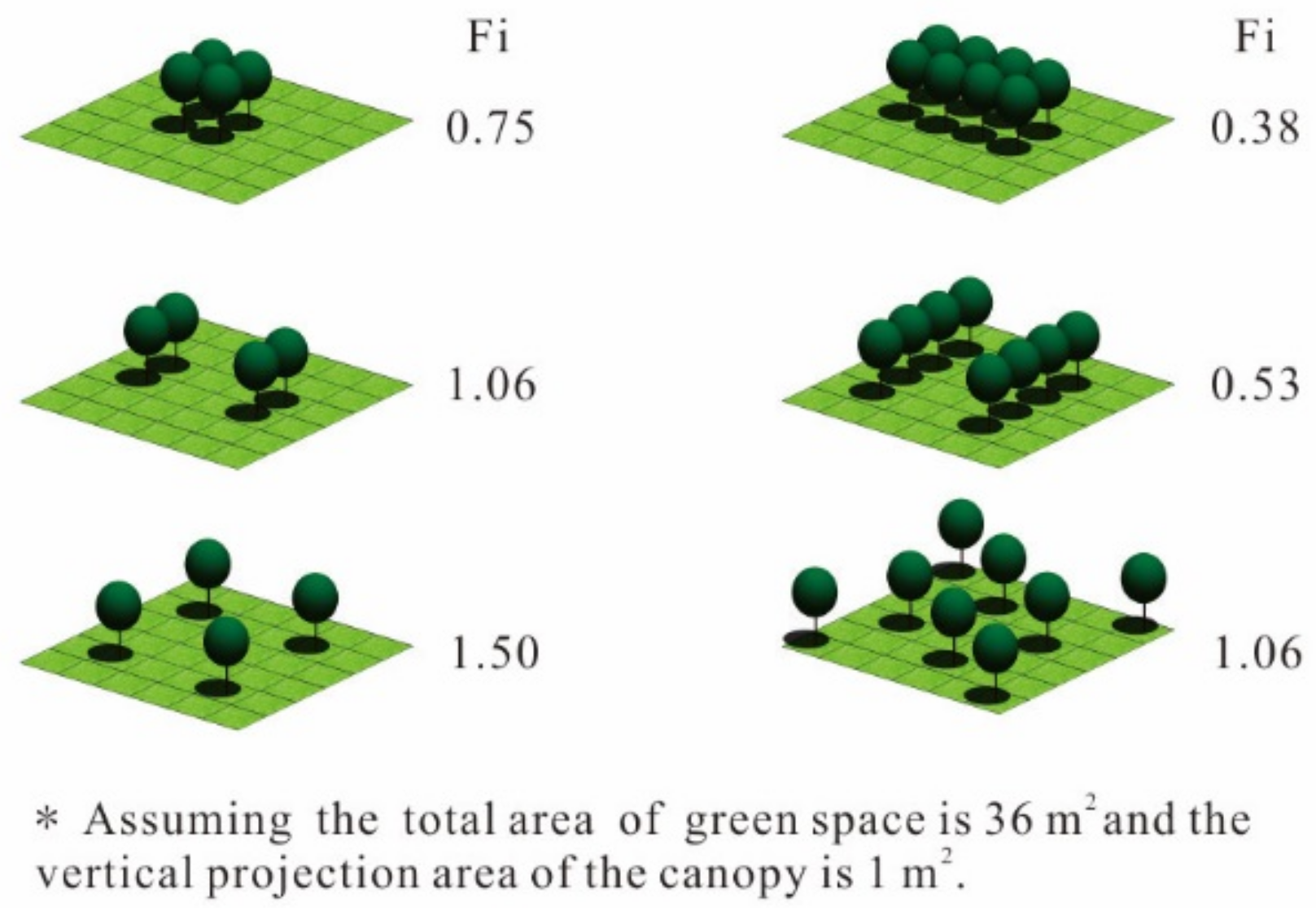
where is the distance index for landscape type i which only considers the influence of the number of patches in the separation of the landscape distribution, is the area index for landscape type i which represents the cover ratio of landscape type i and in this study refers to the cover ratio of trees. Ni is the number of the patches, i.e., the number of groups of trees, and Ai is the area of landscape type i (m2). The large value of Fi implies the patches are far from each other. Figure 2 shows that the value of Fi increases with increasing number of patches and decreases with increasing area of the patches. This index reflects the degree of separation of landscape distribution and was introduced to study the influence of the aggregation distribution of trees on microclimate.
2.2. Thermal Comfort Parameters
To study the influence of green spaces on thermal comfort, two parameters were considered: the mean radiant temperature (MRT) and the predicted mean vote (PMV).
MRT is one of the most important meteorological parameters that is used to evaluate people’s thermal comfort. It is affected by the total amount of radiation absorbed by the human body and is directly influenced by urban geometry and surface materials, particularly under high solar radiation [27,46,47]. MRT is defined as:
where σB = 5.67 × 10⁻⁸ is the Stefan-Boltzmann constant (W/(m2·K4), Et(z), Dt(z), It(z) are the incoming long wave radiation (W/m2), incoming direct short wave radiation (W/m2) and incoming diffuse short wave radiation (W/m2), respectively. αk is the absorption coefficient of the human body for short wave radiation and is set to 0.7, and εp is the emission coefficient of the human body and is set to 0.97.
The predicted mean vote (PMV) is based on the heat balance of the human body, which can be used to predict the general thermal sensation and degree of discomfort of people exposed to indoor thermal environments [48]. It is also used as the outdoor thermal comfort index relating the energy balance of the human body to the personal feeling of people, taking into consideration the influence of four meteorological parameters (air temperature, mean radiant temperature, wind speed and relative humidity) and personal factors (heat resistance of clothing and human activity) on thermal comfort. PMV, which ranges from −4 (very cold) to +4 (very hot) [49], is defined as:
where M is the metabolic rate (W/m2), W is the external work (W/m2), ADu is the surface area of human skin (m2), Ed and ESW are the heat loss by moisture diffusion and evaporation of sweat (W), respectively. Ere and L are the latent heat loss of respiration and sensible heat loss of respiration (W), respectively. R and C are radiant heat exchange and convective heat exchange (W), respectively. ta is the air temperature (°C). tr is the mean radiant temperature (°C). va is the wind speed (m/s). rh is the relative humidity (%). Icl is the clothing insulation (clo). In this study, body parameters were defined according to a standard human [50], except that the clothing insulation was decreased from the standard value 0.9 clo to 0.5 clo because simulations were performed for hot summer conditions.
Both MRT and PMV were calculated based on parameters directly obtained from ENVI-met. The selected height for the calculations was defined at 1.4 m (pedestrian height).
2.3. Description of the Investigated Cases
To achieve higher efficiency of land usage and meet the residential needs, the layout of urban residential districts generally adopts aligned and staggered forms or free irregular forms. Taking as an example the city of Nanjing, China, based on the analysis of building layout (morphology) in the main urban area, it was found that residential buildings are mainly of the 6-story plate-type and the layout of plate-type residential buildings is mainly parallel, as shown in Figure 3.
Based on the statistics of residential building size and street width [51,52], an idealized residential district model was set up as shown in Figure 4 (highlighted in brown). It is made of blocks aligned along the north-south direction and the height, length and width of each six-story building are 18 m, 48 m and 12 m, respectively. The distance between buildings along a north and south direction is 24 m, and the distance between east and west is 16 m, resulting in a planar area index (ratio between the planar area of buildings and the total lot area) λp = 0.25. The widths of roads in residential district and main traffic roads are 24 m and 32 m, respectively. Considering the impact of the model boundary on the result of the simulation area, one half of a block was added around the residential district area. The final simulation area (computational domain) was 416 m × 448 m (see Section 2.4.1).
Both green quantity and green structure indices (see Section 2.1) were used to develop several scenarios of different green spaces distribution and to evaluate the influence on microclimate. Specifically, a green space with an area of 48 m × 16 m was placed between North-South adjacent residential buildings. Four typical cases that are commonly used in the residential green spaces in Nanjing were set up and numbered A-D as shown in Table 2. In addition, a case without green space was also simulated as the base case (“non-green scenario” hereafter).
2.4. ENVI-Met Model Description
2.4.1. Computational Domain
The three-dimensional simulation area (computational domain) had a dimension of 416 m × 448 m and a vertical height of 40 m. The area was meshed using a rectangular grid with 279,552 cells. The grid resolution was 4 m × 4 m in the x and y direction as commonly applied in previous studies (see for example [39,53]), and the vertical size of the cells in the z direction was 2 m (equidistant), except for the lowest five cells which was 0.4 m (assuring at least 3 cells up to pedestrian level of 1.4 m) in order to increase the accuracy near the surfaces where larger gradients were expected. The lower vertical size of the cells close to the ground has the advantage that the exchange processes between atmosphere and ground, which have a substantial influence on the microclimate at ground level and are most interesting from a bio-meteorological point of view, can be simulated more accurately [54]. To improve model accuracy and avoid numerical errors caused by model boundary interference with internal model dynamics, ten nested grids were employed.
Two receptors (P and Q) were selected inside the residential model area to evaluate the temporal variation of meteorological parameters and pollutant concentration (see Figure 4). Both receptors were located at street intersections. Receptor P was selected because it is located downstream of vegetation with respect to the approaching wind and thus it is expected to better reflect the variation of thermal environment under different vegetation configurations. Receptor Q was located close to the side where the approaching wind enters the residential district and close to the pollutant source, where PM10 concentration is supposed to be high.
For each case, ENVI-met was run for a 48 h period, starting at 06:00 a.m. 22 June to 06:00 a.m. 24 June, with model output every hour, using the configuration parameters described below and listed in Table 3. The first hour (6:00 a.m.), for which the input parameters were input by the user, was discarded and the analysis started from 07:00 am. Further, the ENVI-met model required spin-up time before the flow field reached stability, and the results of the first several hours were inaccurate as can be seen in the temporal profiles in the results section, so the analysis of contours and data focused on the second next day (23 June) of simulation.
2.4.2. Meteorological Parameters
Flow solver in the atmospheric system is based on the Reynolds Averaged Navier-Stokes (RANS) equations, and the standard k-ε model is used for the turbulence closure [26]. Meteorological parameters (i.e., temperature and relative humidity) used for model initialization corresponded to those of a typical summer day in June in Nanjing [55]. Specifically, the wind speed at 10 m above the ground level was set to 3 m/s, with a wind direction of 135° (see Table 3).
2.4.3. Pollutant Dispersion
ENVI-met uses the Eulerian approach to study the dispersion of pollutants, allowing simulation of pollutant dispersion including particles, passive gases and reactive gases. Dispersion of pollutants is calculated using the standard advection-diffusion governing equation. By adding source and sink terms in the equation, local processes that influence the change in concentration of local pollutant source or the deposition of particles can be parameterized [26]. As a result of gravitational forces, particles deposit on different surfaces, including building walls, roofs, vegetation and soil, also known as particle sediment, which is considered in this model. The pollution source in ENVI-met is defined in the model domain and can be line-, point- or area sources with hourly emission rates. Traffic emissions can be calculated by multiplying an emission factor (g/km vehicle) with the prevailing traffic intensity (vehicle/s). Here, line sources of PM10 were considered, with a constant source emission strength of 0.1 mg/m·s that corresponds to an average emission factor of 0.347 g/km per vehicle according to the tunnel test of vehicles in Nanjing [56], with a car speed of 40 km/h and 25 cars per km. To mimic mixing by traffic-induced turbulence, emission was distributed over the entire dimension of the traffic lane at the height of 0.4 m. By fixing the emission strength for all the cases, it was possible to isolate the impact of different types of vegetation on microclimate and air quality. The source position is shown in Figure 4.
2.4.4. Vegetation
The equations adopted to model vegetation in ENVI-met are mostly described in Bruse and Fleer [26], while further developments have been collated in the model webpage (http://www.envi-met.info/doku.php?id=root:start). In summary, vegetation is treated as a one-dimension column. The presence and physical characteristics (shape and height) of vegetation are parameterized using the leaf area density (LAD, m2/m3) which is defined as the total leaf area divided by the total volume of vegetation. The height of the plant zp is divided into ten layers (whose height is defined as zpl = zp/10) and a leaf area density value is assigned to each layer. The direct heat flux, the evaporation flux and the transpiration flux are considered in the interactions between the vegetation and the surroundings. The influence of LAD on atmospheric transport is simulated by including additional terms in the prognostic equations using source/sink terms describing heat, humidity and momentum exchange. For shading calculation, vegetation is treated as a turbid medium and the attenuation coefficient is the function of the optical path of the solar beam through the canopy and LAD. However, the attenuation of the diffuse radiation by vegetation is not yet taken into account. In addition, the LAD is also an important parameter in the calculation of the mass of particles deposited. The filtering capacity of vegetation is defined as a sink term in the dispersion equation, and the aerodynamic resistance and sublayer resistance (quasi-laminar resistance) are considered in the calculation of particle deposition velocity [57].
Since the ENVI-met database does not contain proper LAD values of trees present in residential districts, the analytical method developed by Lalic and Mihailovic [58] was used, as recommended by the software developer. They presented a general method to obtain the LAD profile based on a few parameters: height, the maximum LAD and the height of maximum LAD. In this study, the common tree species Ulmus pumila L. was chosen and the height of trees, the maximum value of LAD and the height of maximum LAD were assumed to be 8 m, 1 m2/m3 and 5 m, respectively. Such a way to represent vegetation is not accurate, but it is the best approximation ENVI-met currently allows. LAD values of grass and shrub were taken from the local ENVI-met database; since their heights (0.4 m and 1.2 m, respectively) were strictly linked to the vertical grid resolution (0.4 m), one single value was employed instead of a profile (Table 4).
3. Results and Discussion
3.1. The Impact of Green Space Layout on Thermal Comfort
3.1.1. Air Temperature and Humidity
To evaluate the variation of temperature and relative humidity at pedestrian height (1.4 m), hourly profiles are shown at point P starting from 7:00 on 22 June to 6:00 on 24 June (Figure 5). The maximum temperature and minimum relative humidity occurs at 15:00, while the minimum temperature and maximum relative humidity occurs at around 5:00. It can be noted that between 12:00 and 16:00, Case A (grass) experiences higher temperature and lower relative humidity due to the lower evaporation and solar radiation absorption in comparison to shrubs and trees present in the other cases.
The spatial distribution of temperature in the whole computational domain at pedestrian height at 14:00 on 23 June (Figure 6) shows that the different green types and layouts present in the residential district do not have different influences on the surrounding temperature. In fact, the distribution of the temperature fields are quite similar, with temperatures between 24 °C and 27 °C and the highest temperature in areas surrounding the district. Due to the larger solar radiation absorption and water evaporation by vegetation in Cases B, C and D (as already shown in Figure 5), the district average temperatures are lower than those found in Case A.
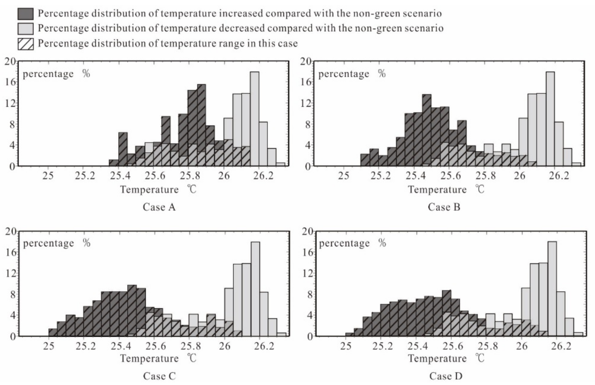
The spatial average temperature values, calculated by averaging the temperatures at all the pedestrian cells in the residential district, are 25.8 °C (Case A) and 25.5 °C (Cases B, C and D), while the average temperature in the non-green scenario is 26 °C. This shows that the cooling effect in the residential district depends on the green types and layout. Thus, to better compare the cooling effect of the different cases, Figure 7 shows the percentage distribution of the temperature range that counts up the temperature data within each cell at pedestrian height. It can be observed that all cases had a great cooling effect compared with the non-green scenario. The minimum and maximum temperatures in Case A (i.e., 25.4 °C and 26.2 °C, respectively) are higher than those of the other three cases (about 25.1 °C and 26.1 °C). It can thus be concluded that: (i) the cooling effect of the combination of grasses and shrubs (Case B) and grasses and trees (Cases C and D) is better than that of grass alone (Case A); and (ii) the temperature range of Cases C and D is more evenly distributed and the area of temperatures below 25.2 °C is larger than that in Case B, which means trees had the largest cooling effect.
Finally, to locally compare the cooling effects of different green types and layouts, Figure 8 shows the detailed spatial distribution of temperature and relative humidity in the district area. The distribution of the low temperature area is consistent with the area where relative humidity is high. The clear cooling effect and evaporation effect of trees, which makes the temperature lower and humidity higher, causes the increase in the relative humidity. The area where the air temperature is below 25.2 °C is mainly concentrated on the north side of the buildings, where the local cooling effect of Case B (grass and shrubs) is not pronounced compared with that of Cases C and D (grass and trees). In addition, the effect of local cooling of tree-grass structure is related to the degree of aggregation, as the concentrated trees in Case D placed in the center of the green space enhanced the temperature difference between the north and south sides of the buildings.
3.1.2. Wind Speed
Figure 9 shows the hourly profiles of wind velocity at point P. For all the cases, the profile gradually decreases and reaches the minimum daily value at 8:00. After that it gradually increases again until the wind velocity reaches the maximum daily value at 16:00, then decreases again. The wind speed in Case A (grass) is higher since the grass had less effect in blocking the wind than shrubs and trees (Cases B, C and D). Please note that the reason for the decrease in wind speed during the first few hours is due to the fact that the flow field has not reached stability (spin-up effect mentioned in Section 2.4.1). Neglecting the first day (22 June), the daily variation of the wind speed can be associated with the temperature variation (Figure 5), i.e., when the air temperature increases, the wind speed increases as well. The plausible explanation is that solar radiation causes the ground to heat up and enhances vertical convection.
Figure 10 shows the percentage distribution of wind speed in the residential district. On average, wind speeds in Cases A–D are 1.33 m/s, 1.08 m/s, 1.09 m/s and 1.14 m/s, respectively, while in non-green scenario, the wind speed is 1.41 m/s. Over 61% of the residential district area in Case A experienced a wind speed above 1.3 m/s, while in Cases B, C and D the areas are 17%, 21% and 32%, respectively, due to an increasing blocking effect of vegetation compared with the non-green scenario.
Finally, to compare the local effect of the different green layouts, Figure 11 shows the detailed contours of wind speed in the residential district. In general, the wind speed in the north area is relatively lower than in the south area due to the obstacle effect of buildings and vegetation. By analyzing in detail Cases B, C and D, the wind speed distribution in Case B is generally lower and uniform due to the continuous shrub arrangement, and the wind speed is higher in the center of the green space where the grass is located and thus exerts less resistance to the wind. In Case C, due to the distributed trees placed around the green space, the ventilation in the central area is enhanced compared with the other two cases, while the east-west ventilation in the south side of the buildings is affected. In Case D (concentrated trees placed in the center of the green space), lower wind speed zones occurs in the north side of the buildings and the center of the green space due to the larger blocking effect.
3.1.3. Mean Radiant Temperature and Predicted Mean Vote
Figure 12 shows the hourly variation of MRT and PMV at point P. The blue area in the figure is the thermal comfort zone, while the thermal sensation corresponding to the red zone is evaluated as hot. The areas below the blue zone, between the red and blue area and above the red area, mean cool, warm and very hot, respectively. It can be seen that there is a little difference between the different cases, and profiles of MRT and PMV are qualitatively similar. During the day, MRT reaches about 76 °C, while it drops to 10 °C at night. MRT increases from 6:00 and reaches two peaks at 9:00 and 17:00, which means that there might be a radiant load on building facades. As for PMV, the hours from 19:00 on 22 June to 6:00 on the next morning are below the blue zone and from 7:00 to 18:00 they are in the shape of “M”. On 23 June, only the hours 7:00, 18:00 and 19:00 are in the comfort zone, while 8:00–12:00 are warm and 13:00–17:00 are very hot. In particular, at 12:00 and 15:00, the hot feeling zone is reached. In general, Case A (grass) experiences a larger fluctuation of PMV, i.e., the upper and lower limits of PMV are respectively higher and lower than other cases.
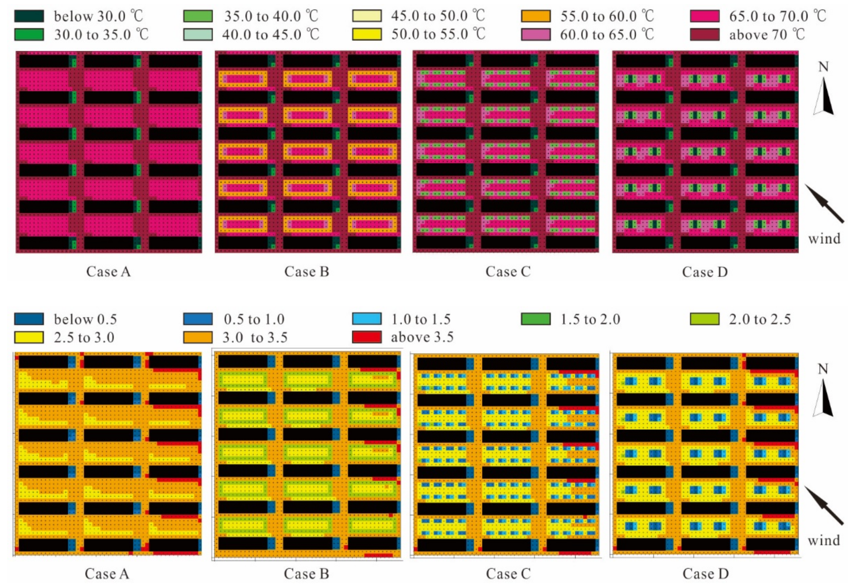
Figure 13 shows the MRT and PMV distribution in the residential district at pedestrian height on 23 June at 14:00. The average MRTs and PMVs in the non-green scenario are 70 °C and 3.3, respectively (not shown here); in Cases A–D the average MRTs decrease to 67 °C, 64 °C, 62 °C and 63 °C, respectively, and the average PMVs to 3.0, 2.8, 2.6 and 2.7, respectively. Compared with the shrub-grass structure (Case B) and tree-grass structure (Cases C and D), the single grass (Case A) structure has relatively less effect in improving the comfort. In particular, trees play a significant role in improving the local thermal comfort with a reduction of PMV to about 0.5 under tree shading.
3.2. The Impact of Green Space Layout on PM10 Concentration
To study the hourly variation of PM10 concentration in the residential district, profiles at point Q and contours are analyzed. Figure 14 presents the hourly variation of PM10 concentration at point Q, showing that the concentration during the day is lower than that at night. The valleys and peaks of 22 June and 23 occurs at about 13:00 and 19:00, respectively. The valleys show a “U” shape, which mean that the PM10 concentration is maintained at a relatively low level within a couple of hours. This is because the higher temperature (Figure 5) and wind speed (Figure 9) during the day cause the particles to disperse more rapidly. Then PM10 concentration decreases, reaching the minimum at 13:00 when the temperature is the maximum. Further, the humidity during the day is lower than that at night (Figure 5), and its increase results in the increase of air density at night, which causes the deposition velocity to decrease and PM10 concentration to increase.
Figure 15 shows the contours of the PM10 concentration and wind speed in the residential district; the interval between concentration contour lines is 2 μg/m3 and the initial contour line in the northwest residential area is 4 μg/m3. The average PM10 concentrations at pedestrian height are 10.7 μg/m3 (Case A), 11.0 μg/m3 (Case B), 10.9 μg/m3 (Case C) and 10.9 μg/m3 (Case D), while in the non-green scenario, the value is about 10.7 μg/m3. In general, the contours are similar for all the cases investigated. In particular, PM10 concentration is higher at the upwind side (south-east) of the residential district, while a low PM10 concentration area occurs at the northwest side (downwind). The wind speed contours show that the ventilation effect on the south sides (those exposed to the wind) of the buildings is better than that on north sides (downwind), leading to uneven concentration distributions. The ventilation is a consequence of the vortices which developed within the street canyons for such an array of packing density λp = 0.25, which is considered a border case between sparse and compact cities [59,60]. Thus, the pollutant accumulated within the street canyons is closer to the pollutant source upwind with poor pollution transport downwind. The ventilation gets worse in the presence of vegetation as the concentration distribution suggests that the aerodynamic effect seemed to prevail over the filtering capacity [18,19,20,21,22].
To further show the effect of vegetation on pollutant dispersion, as an example Figure 16 shows that, for Case A, the area where the PM10 concentration is below 10 μg/m3 almost accounts for 64% and the maximum PM10 concentration in the residential district is about 50 μg/m3.
4. Discussion
The analysis has shown that the effects of vegetation on microclimate and air quality are not only related to the green cover but also to the vegetation types and layout of trees.
In particular, even though Cases A (only grass) and B (grass and shrubs) had the same maximum value (100%) of green cover ratio (Cg) and grass and shrubs cover ratio (Gg), they did not show the maximum cooling effect and the best thermal comfort. Instead, the combination of grass and trees (Cases C and D), which had the same Cg and lower Gg of Cases A and B, led to an average temperature reduction of approximately 0.5 °C compared with the non-green scenario, showing trees play a significant role in cooling, suggesting that Cg and Gg cannot be employed alone to evaluate the cooling effect. In this regard, the new ecological landscaping plot ratio Rg proposed here was found to be appropriate in evaluating the cooling effect of vegetation as larger Rg (in Cases B, C and D) showed a larger cooling effect, with a PMV reduction of about 20% compared with the non-green scenario.
Further, these effects depend on the degree of separation of landscape distribution (expressed by the landscaping isolation index Fi). In fact, the local cooling effect of concentrated structure of vegetation in Case D (lower Fi) was larger than the distributed structure in Case C during the day, even though the temperature distribution was relatively uneven, while in Case C it was more uniform. Thus, it can be concluded that reducing the landscaping isolation index (through a concentrated structure of vegetation) helps to create a larger shading area and improves the local cooling effect of trees, while increasing it (through a distributed structure of vegetation) is beneficial for uniform temperature and improve the general thermal comfort.
The pollutant concentration distribution was closely related to temperature, humidity and air flow. The effect of shrub-grass (Case B) and tree-grass (Cases C and D) structures on wind blocking was slightly stronger than the single grass structure (Case A), even though it was characterized by the same green cover ratio (Cg). In fact, while Case A provided the same average PM10 concentration compared to the non-green scenario, with increasing ecological landscaping plot ratio Rg in the other cases, the average wind speed in the area worsened the ventilation due to the presence of continuous shrubs and trees, thus increasing average PM10 concentration up to about 3%. Further, under the same values of green quantity indices, with higher Fi in Case C, i.e., looser distribution of trees, the effect on wind blocking was relatively small compared with the concentrated trees in Case D. This suggests that green spaces with a low ecological landscaping plot ratio Rg and high landscaping isolation index Fi are expected to have lower effects on wind blocking and thus to be more beneficial for pollutant dilution.
5. Conclusions
This paper attempts to make a link between green indices and the microclimate in idealized residential areas representing typical districts of Nanjing, China. Modeling simulations were performed using ENVI-met for different scenarios of vegetation types and layouts. The main general conclusions are summarized below:
- under the same green cover ratio (i.e., the same quantity of all types of vegetation), the reduction of grass and shrub cover ratio (i.e., the quantity of grass and shrubs), replaced by trees, has a little impact on thermal comfort, wind speed and air pollution, in addition to increasing the leisure space for occupants;
- a low ecological landscaping plot ratio (which expresses the weight of carbon dioxide absorption and is larger in the presence of trees) is preferable due to a lower wind blocking by vegetation and thus to the enhancement of ventilation and air quality;
- a low landscaping isolation index (thorough a concentrated structure of vegetation) helps to create a larger shading area and improve the local cooling effect of trees, while increasing it (through a distributed structure of vegetation) is beneficial for uniform temperature and to improve the general thermal comfort.
In summary, in conjunction with a low landscaping plot ratio, a high landscaping isolation index enhances the capability of local cooling and improves the general thermal comfort as the temperature is uniformly distributed within the study area, and diminishes the wind blocking by vegetation improving the air quality. This paper shows that the effect of vegetation on microclimate and air quality is complex, and should be analyzed using several green indices which take into account not only the total area covered by vegetation but also its layout and degree of aggregation.
Acknowledgments
The research was supported by the key project funded by the National Science Foundation of China on “Urban form-microclimate coupling mechanism and control”, Grant No. 51538005.
Author Contributions
Z.G. and W.D. were responsible for the study design and supervision. L.R. wrote the manuscript, performed the model simulation and conducted data analysis; J.S. contributed in the data analysis; R.B. revised the paper and wrote sections of the manuscript. All authors contributed to the discussion of the results and have read and approved the final manuscript.
Conflicts of Interest
The authors declare no conflict of interest.
References
- Maleki, H.; Sorooshian, A.; Goudarzi, G.; Nikfal, A.; Baneshi, M.M. Temporal profile of PM10 and associated health effects in one of the most polluted cities of the world (Ahvaz, Iran) between 2009 and 2014. Aeolian Res. 2016, 22, 135–140. [Google Scholar] [CrossRef]
- Chen, L.; Shi, M.; Gao, S.; Li, M.; Zhang, H.; Sun, Y.; Bai, Z.; Wang, Z. Assessment of population exposure to PM2.5 for mortality in China and its public health benefit based on BenMAP. Environ. Pollut. 2016, 221, 311–317. [Google Scholar] [CrossRef]
- Chen, R.; Hu, B.; Liu, Y.; Xu, J.; Yang, G.; Xu, D.; Chen, C. Beyond PM2.5: The role of ultrafine particles on adverse health effects of air pollution. Biochim. Biophys. Acta 2016, 1860, 2844–2855. [Google Scholar] [CrossRef]
- Kumar, P.; Morawska, L.; Birmili, W.; Paasonen, P.; Hu, M.; Kulmala, M.; Harrison, R.M.; Norford, L.; Britter, R. Ultrafine particles in cities. Environ. Int. 2014, 66, 1–10. [Google Scholar] [CrossRef] [Green Version]
- Beevers, S.D.; Westmoreland, E.; de Jong, M.C.; Williams, M.L.; Carslaw, D.C. Trends in NOx and NO2 emissions from road traffic in Great Britain. Atmos. Environ. 2012, 54, 107–116. [Google Scholar] [CrossRef]
- Michiels, H.; Mayeres, I.; Int Panis, L.; De Nocker, L.; Deutsch, F.; Lefebvre, W. PM2.5 and NOx from traffic: Human health impacts, external costs and policy implications from the Belgian perspective. Transp. Res. Part D Transp. Environ. 2012, 17, 569–577. [Google Scholar] [CrossRef]
- Chen, R.; Pan, G.; Zhang, Y.; Xu, Q.; Zeng, G.; Xu, X.; Chen, B.; Kan, H. Ambient carbon monoxide and daily mortality in three Chinese cities: The China Air Pollution and Health Effects Study (CAPES). Sci. Total Environ. 2011, 409, 4923–4928. [Google Scholar] [CrossRef] [PubMed]
- Akbari, H.; Rose, L.S.; Taha, H. Analyzing the land cover of an urban environment using high-resolution orthophotos. Landsc. Urban Plan. 2003, 63, 1–14. [Google Scholar] [CrossRef]
- Abhijith, K.V.; Kumar, P.; Gallagher, J.; McNabola, A.; Baldauf, R.; Pilla, F.; Broderick, B.; Di Sabatino, S.; Pulvirenti, B. Air pollution abatement performances of green infrastructure in open road and built-up street canyon environments—A review. Atmos. Environ. 2017, 162, 71–86. [Google Scholar] [CrossRef]
- Chen, D.; Wang, X.; Thatcher, M.; Barnett, G.; Kachenko, A.; Prince, R. Urban vegetation for reducing heat related mortality. Environ. Pollut. 2014, 192, 275–284. [Google Scholar] [CrossRef] [PubMed]
- Gago, E.J.; Roldan, J.; Pacheco-Torres, R.; Ordó Ez, J. The city and urban heat islands: A review of strategies to mitigate adverse effects. Renew. Sustain. Energy Rev. 2013, 25, 749–758. [Google Scholar] [CrossRef]
- Freer-Smith, P.H.; Beckett, K.P.; Taylor, G. Deposition velocities to Sorbus aria, Acer campestre, Populus deltoides × trichocarpa ‘Beaupré’, Pinus nigra and × Cupressocyparis leylandii for coarse, fine and ultra-fine particles in the urban environment. Environ. Pollut. 2005, 133, 157–167. [Google Scholar] [CrossRef]
- Ould-Dada, Z.; Baghini, N.M. Resuspension of small particles from tree surfaces. Atmos. Environ. 2011, 35, 3799–3809. [Google Scholar] [CrossRef]
- Janhäll, S. Review on urban vegetation and particle air pollution—Deposition and dispersion. Atmos. Environ. 2015, 105, 130–137. [Google Scholar] [CrossRef]
- Tallis, M.; Taylor, G.; Sinnett, D.; Freer-Smith, P. Estimating the removal of atmospheric particulate pollution by the urban tree canopy of London, under current and future environments. Landsc. Urban Plan. 2011, 103, 129–138. [Google Scholar] [CrossRef]
- Nowak, D.J.; Crane, D.E.; Stevens, J.C. Air pollution removal by urban trees and shrubs in the United States. Urban For. Urban Green. 2006, 4, 115–123. [Google Scholar] [CrossRef]
- McDonald, A.G.; Bealey, W.J.; Fowler, D.; Dragosits, U.; Skiba, U.; Smith, R.I.; Donovan, R.G.; Brett, H.E.; Hewitt, C.N.; Nemitz, E. Quantifying the effect of urban tree planting on concentrations and depositions of PM10 in two UK conurbations. Atmos. Environ. 2007, 41, 8455–8467. [Google Scholar] [CrossRef]
- Buccolieri, R.; Santiago, J.-L.; Rivas, E.; Sanchez, B. Review on urban tree modelling in CFD simulations: Aerodynamic, deposition and thermal effects. Urban For. Urban Green. 2018, 31, 212–220. [Google Scholar] [CrossRef]
- Buccolieri, R.; Salim, S.M.; Leo, L.S.; Di Sabatino, S.; Chan, A.; Ielpo, P.; de Gennaro, G.; Gromke, C. Analysis of local scale tree–atmosphere interaction on pollutant concentration in idealized street canyons and application to a real urban junction. Atmos. Environ. 2011, 45, 1702–1713. [Google Scholar] [CrossRef]
- Jeanjean, A.; Buccolieri, R.; Eddy, J.; Monks, P.; Leigh, R. Air quality affected by trees in real street canyons: The case of Marylebone neighbourhood in central London. Urban For. Urban Green. 2017, 22, 41–53. [Google Scholar] [CrossRef]
- Santiago, J.L.; Rivas, E.; Sanchez, B.; Buccolieri, R.; Martin, F. The impact of planting trees on NOx concentrations: The case of the Plaza de la Cruz neighborhood in Pamplona (Spain). Atmosphere 2017, 8, 131. [Google Scholar] [CrossRef]
- Vos, P.E.J.; Maiheu, B.; Vankerkom, J.; Janssen, S. Improving local air quality in cities: To tree or not to tree? Environ. Pollut. 2013, 183, 113–122. [Google Scholar] [CrossRef] [PubMed]
- Shashua-Bar, L.; Hoffman, M.E. The green CTTC model for predicting the air temperature in small urban wooded sites. Build. Environ. 2002, 37, 1279–1288. [Google Scholar] [CrossRef]
- Lindberg, F.; Holmer, B.; Thorsson, S. SOLWEIG 1.0—Modelling spatial variations of 3D radiant fluxes and mean radiant temperature in complex urban settings. Int. J. Biometeorol. 2008, 52, 697–713. [Google Scholar] [CrossRef] [PubMed]
- Matzarakis, A.; Rutz, F.; Mayer, H. Modelling radiation fluxes in simple and complex environments—Application of the Rayman model. Int. J. Biometeorol. 2007, 51, 323–334. [Google Scholar] [CrossRef] [PubMed]
- Bruse, M.; Fleer, H. Simulating surface–plant–air interactions inside urban environments with a three dimensional numerical model. Environ. Model. Softw. 1998, 13, 373–384. [Google Scholar] [CrossRef]
- Ali-Toudert, F.; Mayer, H. Numerical study on the effects of aspect ratio and orientation of an urban street canyon on outdoor thermal comfort in hot and dry climate. Build. Environ. 2006, 41, 94–108. [Google Scholar] [CrossRef]
- Fahmy, M.; Sharples, S. On the development of an urban passive thermal comfort system in Cairo, Egypt. Build. Environ. 2009, 44, 1907–1916. [Google Scholar] [CrossRef]
- Maggiotto, G.; Buccolieri, R.; Santo, M.A.; Leo, L.S.; Di Sabatino, S. Validation of temperature-perturbation and CFD-based modelling for the prediction of the thermal urban environment: The Lecce (IT) case study. Environ. Model. Softw. 2014, 60, 69–83. [Google Scholar] [CrossRef]
- Yang, X.; Zhao, L.; Bruse, M.; Meng, Q. Evaluation of a microclimate model for predicting the thermal behavior of different ground surfaces. Build. Environ. 2013, 60, 93–104. [Google Scholar] [CrossRef]
- Hofman, J.; Samson, R. Biomagnetic monitoring as a validation tool for local air quality models: A case study for an urban street canyon. Environ. Int. 2014, 70, 50–61. [Google Scholar] [CrossRef] [PubMed]
- Krüger, E.L.; Minella, F.O.; Rasia, F. Impact of urban geometry on outdoor thermal comfort and air quality from field measurements in Curitiba, Brazil. Build. Environ. 2011, 46, 621–634. [Google Scholar] [CrossRef]
- Morakinyo, T.E.; Lam, Y.F.; Hao, S. Evaluating the role of green infrastructures on near-road pollutant dispersion and removal: Modelling and measurement. J. Environ. Manag. 2016, 182, 595–605. [Google Scholar] [CrossRef]
- Nikolova, I.; Janssen, S.; Vos, P.; Vrancken, K.; Mishra, V.; Berghmans, P. Dispersion modelling of traffic induced ultrafine particles in a street canyon in Antwerp, Belgium and comparison with observations. Sci. Total Environ. 2011, 412–413, 336–343. [Google Scholar] [CrossRef] [PubMed]
- Wania, A.; Bruse, M.; Blond, N.; Weber, C. Analysing the influence of different street vegetation on traffic-induced particle dispersion using microscale simulations. J. Environ. Manag. 2012, 94, 91–101. [Google Scholar] [CrossRef]
- Morakinyo, T.E.; Lam, Y.F. Simulation study of dispersion and removal of particulate matter from traffic by road-side vegetation barrier. Environ. Sci. Pollut. Res. 2016, 23, 6709–6722. [Google Scholar] [CrossRef] [PubMed]
- Samaali, M.; Courault, D.; Bruse, M.; Olioso, A.; Occelli, R. Analysis of a 3D boundary layer model at local scale: Validation on soybean surface radiative measurements. Atmos. Res. 2007, 85, 183–198. [Google Scholar] [CrossRef]
- Chow, W.T.L.; Pope, R.L.; Martin, C.A.; Brazel, A.J. Observing and modeling the nocturnal park cool island of an arid city: Horizontal and vertical impacts. Theor. Appl. Climatol. 2011, 103, 197–211. [Google Scholar] [CrossRef]
- Chow, W.T.L.; Brazel, A.J. Assessing xeriscaping as a sustainable heat island mitigation approach for a desert city. Build. Environ. 2012, 47, 170–181. [Google Scholar] [CrossRef]
- Ng, E.; Chen, L.; Wang, Y.; Yuan, C. A study on the cooling effects of greening in a high-density city: An experience from Hong Kong. Build. Environ. 2012, 47, 256–271. [Google Scholar] [CrossRef]
- Lee, H.; Mayer, H.; Chen, L. Contribution of trees and grasslands to the mitigation of human heat stress in a residential district of Freiburg, Southwest Germany. Landsc. Urban Plan. 2016, 148, 37–50. [Google Scholar] [CrossRef]
- Wu, Z.; Kong, F.; Wang, Y.; Sun, R.; Chen, L. The Impact of Greenspace on Thermal Comfort in a Residential Quarter of Beijing, China. Int. J. Environ. Res. Public Health 2016, 13, 1217. [Google Scholar] [CrossRef]
- Tong, Z. The Study of Quantification Method on Urban Greenspace Configuration. Ph.D. Thesis, Nanjing University, Nanjing, China, 2011. (In Chinese). [Google Scholar]
- Lin, X. Green Building: Ecology, Energy Saving, Waste Reduction, Health; China Architecture & Building Press: Beijing, China, 2007; p. 83. ISBN 9787112092239. [Google Scholar]
- Chen, L.; Fu, B. Analysis of impact of human activity on landscape structure in Yellow River Delta: A case study of Dongying region. Acta Ecol. Sin. 1996, 16, 337–344. (In Chinese) [Google Scholar]
- Qaid, A.; Bin Lamit, H.; Ossen, D.R.; Raja Shahminan, R.N. Urban heat island and thermal comfort conditions at micro-climate scale in a tropical planned city. Energy Build. 2016, 133, 577–595. [Google Scholar] [CrossRef]
- Hoppe, P. The physiological equivalent temperature—A universal index for the biometeorological assessment of the thermal environment. Int. J. Biometeorol. 1994, 43, 71–75. [Google Scholar] [CrossRef]
- Fanger, P.O. Thermal Comfort: Analysis and Applications in Environmental Engineering; Danish Technical Press: Copenhagen, Denmark, 1970. [Google Scholar]
- Jendritzky, G. The atmospheric environment—An introduction. Experientia 1993, 49, 733–738. [Google Scholar] [CrossRef] [PubMed]
- ISO 7730. Ergonomics of the Thermal Environment—Analytical Determinationand Interpretation of Thermal Comfort Using Calculation of the PMV and PPD Indices and Local Thermal Comfort Criteria; International Organization for Standardization: Geneva, Switzerland, 2005. [Google Scholar]
- You, W.; Shen, J.; Ding, W. Improving wind environment of residential neighborhoods by understanding the relationship between building layouts and ventilation efficiency. Energy Procedia 2017, 105, 4531–4536. [Google Scholar] [CrossRef]
- Shen, J.; Gao, Z.; Ding, W.; Yu, Y. An investigation on the effect of street morphology to ambient air quality using six real-world cases. Atmos. Environ. 2017, 164, 85–101. [Google Scholar] [CrossRef]
- Lu, J.; Li, Q.; Zeng, L.; Chen, J.; Liu, G.; Li, Y.; Li, W.; Huang, K. A micro-climatic study on cooling effect of an urban park in a hot and humid climate. Sustain. Cities Soc. 2017, 32, 513–522. [Google Scholar] [CrossRef]
- Huttner, S. Further Develop and Application of the 3D Microclimate Simulation ENVI-Met. Ph.D. Thesis, Johannes Gutenberg-University, Mainz, Germany, 2012. [Google Scholar]
- Weather Data by Location. Energyplus Website. Available online: https://energyplus.net/weather-location/asia_wmo_region_2/CHN//CHN_Jiangsu.Nanjing.582380_CSWD (accessed on 26 January 2018).
- Hu, W.; Zhong, Q. A study on PM10 emission factor of motor vehicle by tunnel test in Nanjing city. CJEE 2009, 3, 1852–1855. (In Chinese) [Google Scholar]
- Bruse, M. Particle filtering capacity of urban vegetation: A microscale numerical approach. Berl. Geogr. Arb. 2007, 109, 61–70. [Google Scholar]
- Lalic, B.; Mihailovic, D.T. An empirical relation describing leaf area density inside the forest for environmental modelling. J. Appl. Meteorol. 2004, 43, 641–645. [Google Scholar] [CrossRef]
- Buccolieri, R.; Sandberg, M.; Di Sabatino, S. City breathability and its link to pollutant concentration distribution within urban-like geometries. Atmos. Environ. 2010, 44, 1894–1903. [Google Scholar] [CrossRef]
- Buccolieri, R.; Wigö, H.; Sandberg, M.; Di Sabatino, S. Direct measurements of the drag force over aligned arrays of cubes exposed to boundary-layer flows. Environ. Fluid Mech. 2017, 17, 373–394. [Google Scholar] [CrossRef]
Figure 1.
Green quantity indices for different green space configurations. Gg: grass and shrub cover ratio; Cg: green cover ratio; Rg: ecological landscaping plot ratio.
Figure 1.
Green quantity indices for different green space configurations. Gg: grass and shrub cover ratio; Cg: green cover ratio; Rg: ecological landscaping plot ratio.

Figure 2.
Examples of the landscaping isolation index Fi for different distribution patterns of trees.
Figure 2.
Examples of the landscaping isolation index Fi for different distribution patterns of trees.

Figure 3.
The layout of buildings (morphology) of typical residential districts in Nanjing, China.
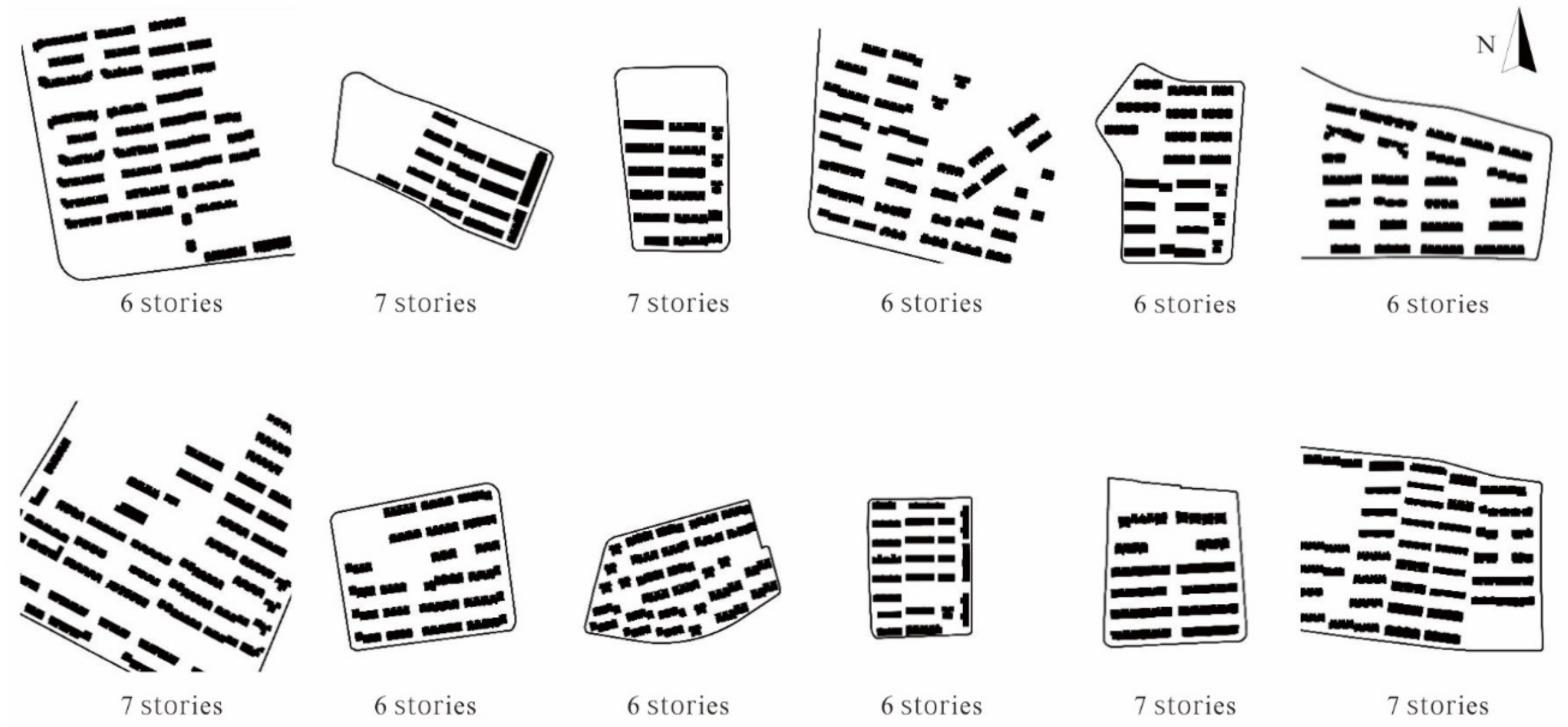
Figure 4.
The idealized residential district area (highlighted in brown) of size 184 m × 200 m, with indication of the position of two receptors (P and Q) and pollutant line sources (dashed lines).
Figure 4.
The idealized residential district area (highlighted in brown) of size 184 m × 200 m, with indication of the position of two receptors (P and Q) and pollutant line sources (dashed lines).

Figure 5.
Temporal profile of temperature and relative humidity at point P.

Figure 6.
Spatial distribution of temperature at pedestrian height on 23 June at 14:00.

Figure 7.
Percentages distribution of temperatures range in residential district at pedestrian height on 23 June at 14:00.
Figure 7.
Percentages distribution of temperatures range in residential district at pedestrian height on 23 June at 14:00.

Figure 8.
Contours of temperature distribution (top) and relative humidity (bottom) in the residential district at pedestrian height on 23 June at 14:00.
Figure 8.
Contours of temperature distribution (top) and relative humidity (bottom) in the residential district at pedestrian height on 23 June at 14:00.
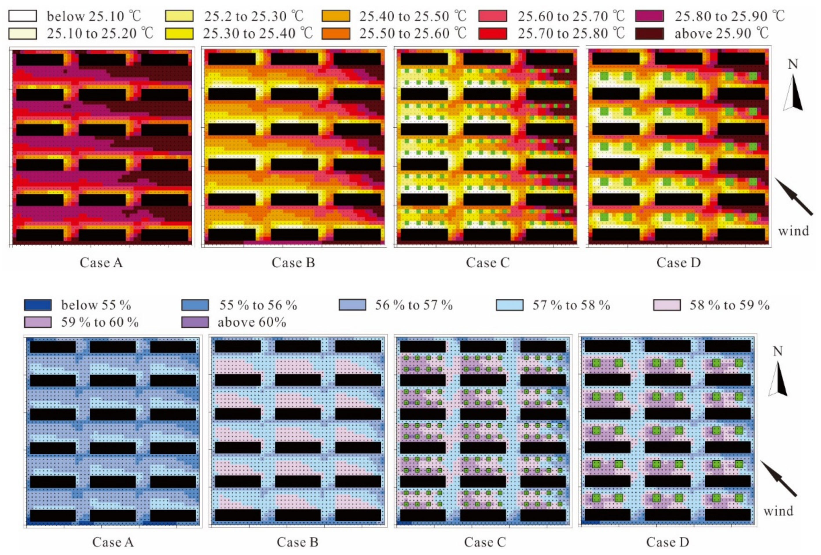
Figure 9.
Temporal profile of wind speed at point P.
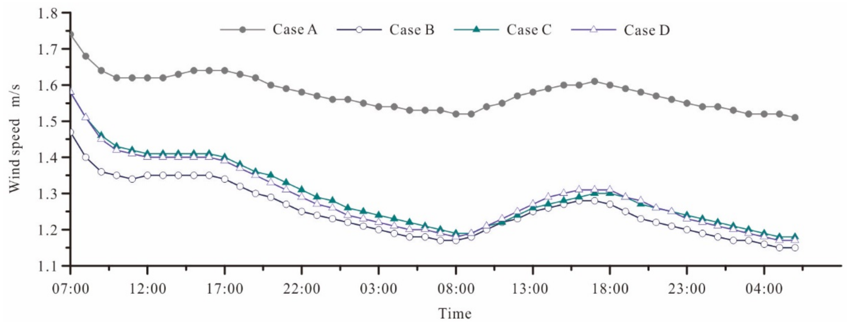
Figure 10.
Percentage distribution of wind speed range in the residential district area at pedestrian height on 23 June at 14:00.
Figure 10.
Percentage distribution of wind speed range in the residential district area at pedestrian height on 23 June at 14:00.
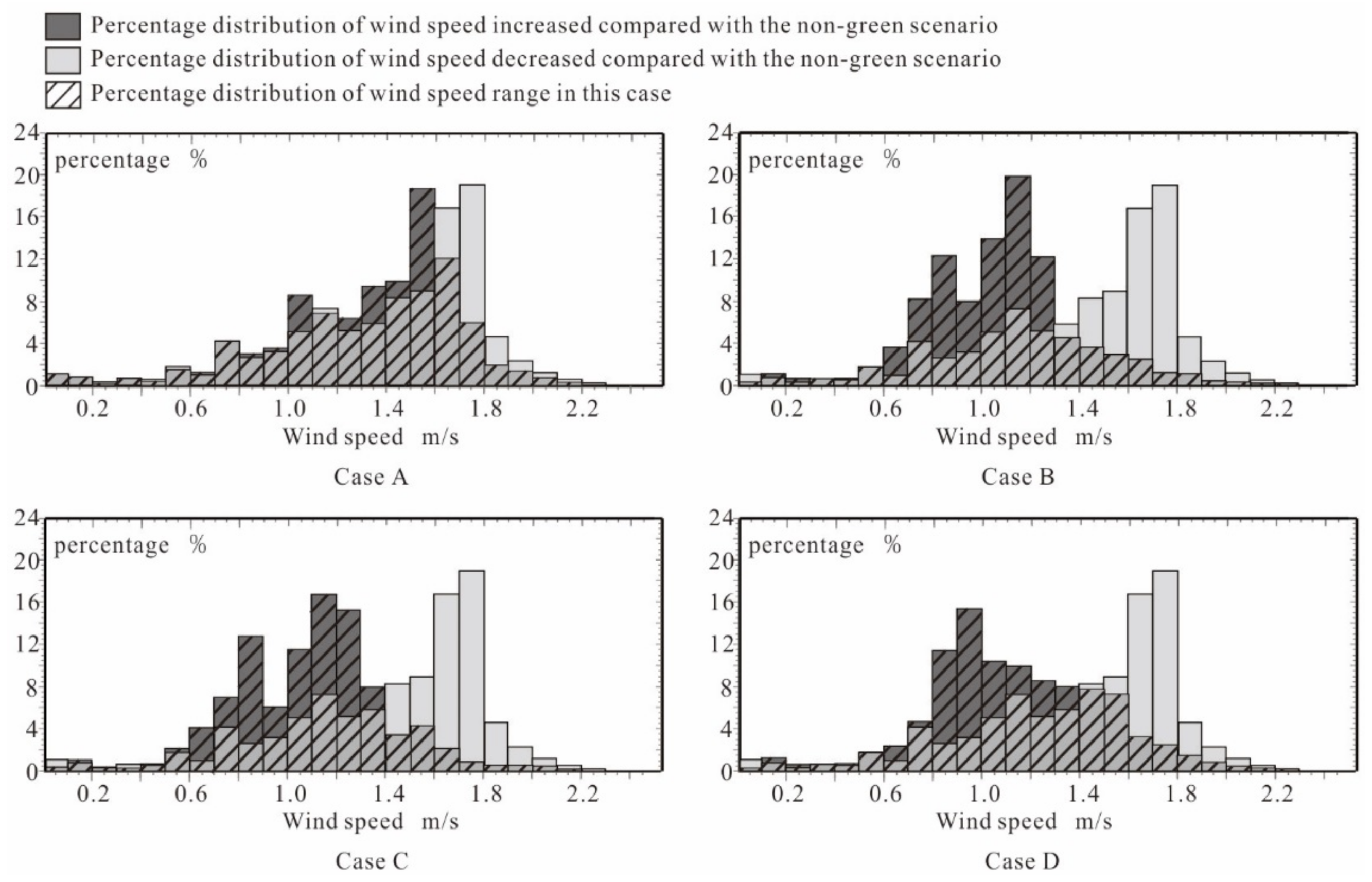
Figure 11.
Contours of wind speed distribution in the residential district at pedestrian height on 23 June at 14:00.
Figure 11.
Contours of wind speed distribution in the residential district at pedestrian height on 23 June at 14:00.

Figure 12.
Temporal profiles of mean radiant temperature (MRT) and predicted mean vote (PMV) at point P.
Figure 12.
Temporal profiles of mean radiant temperature (MRT) and predicted mean vote (PMV) at point P.
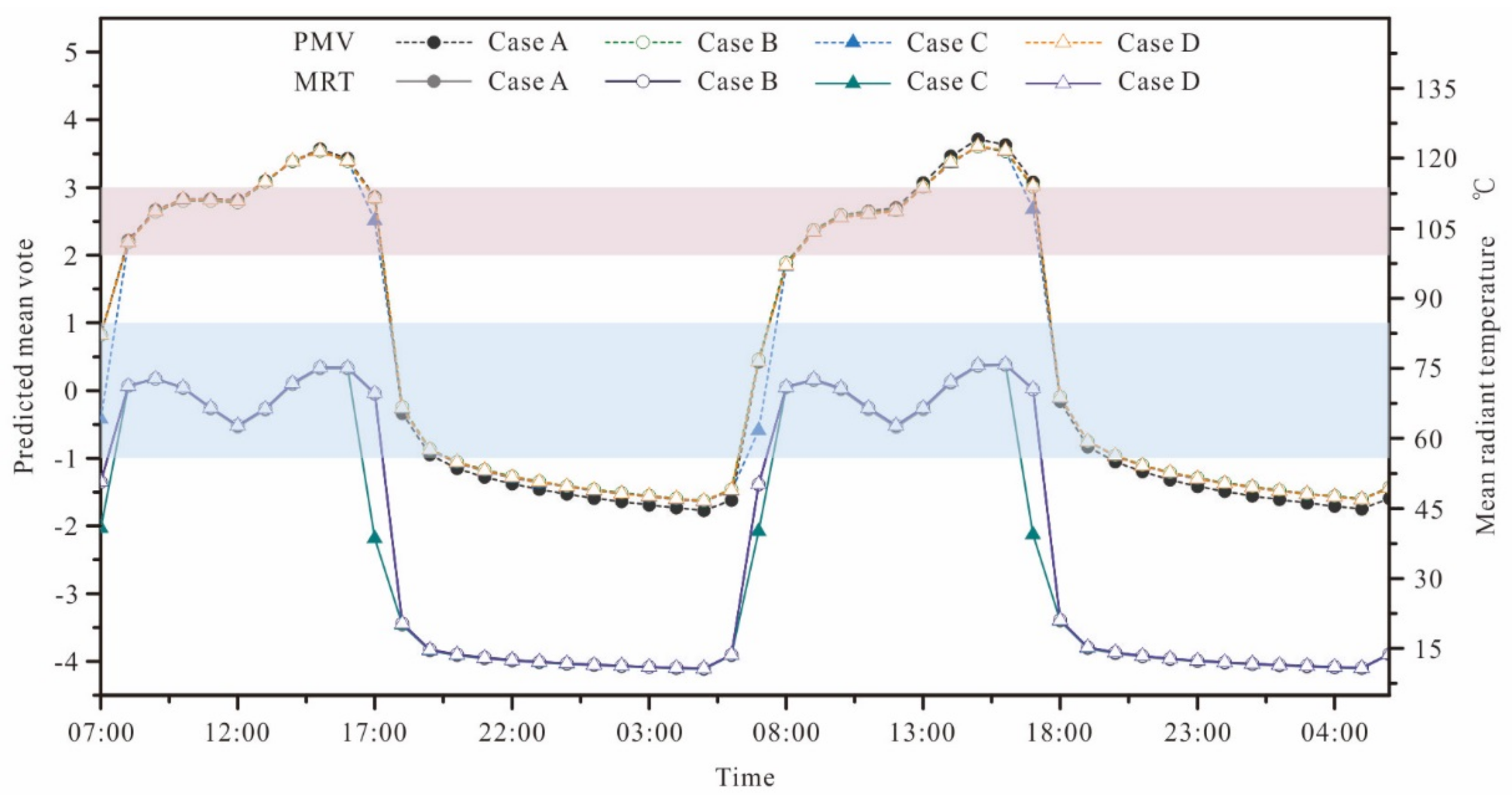
Figure 13.
Contours of MRT (top) and PMV (bottom) at pedestrian height on 23 June at 14:00.

Figure 14.
Temporal profile of PM10 concentration at point Q.

Figure 15.
Contours of PM10 concentration (top) and wind speed (bottom) in the residential area at pedestrian height on 23 June at 19:00.
Figure 15.
Contours of PM10 concentration (top) and wind speed (bottom) in the residential area at pedestrian height on 23 June at 19:00.

Figure 16.
Percentage PM10 concentration range in the residential district at pedestrian height on 23 June at 19:00 (Case A).
Figure 16.
Percentage PM10 concentration range in the residential district at pedestrian height on 23 June at 19:00 (Case A).


Table 1.
The amount of carbon dioxide absorbed by various vegetation types in the 40-year life cycle [44].
Table 1.
The amount of carbon dioxide absorbed by various vegetation types in the 40-year life cycle [44].
| Vegetation Type | CO2 Absorption (kg/m2) | Depth of Soil Cover |
|---|---|---|
| Tree (small broad-leaved trees, coniferous trees) | 600 | >1.0 m |
| Shrub (at least 4 plants per square meter) | 300 | >0.5 m |
| Grass (grass garden, natural weeds, aquatic plants, lawns) | 20 | > 0.3 m |
Table 2.
Investigated cases representing residential districts with different quantity and green structure indices.
Table 2.
Investigated cases representing residential districts with different quantity and green structure indices.
| Case Code | A | B | C | D |
|---|---|---|---|---|
| Description | 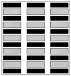 | 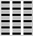 | 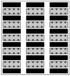 | 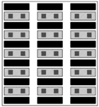 |
| Grass | Grass is placed in the center of green spaces, surrounded by 4 m width shrub | The area consists of grass and distributed trees. The single patch of trees is 4 m × 4 m. | The area consists of grass and concentrated trees. The single patch of trees is 8 m × 8 m. | |
| Green quantity index | Gg = 100% Cg = 100% Rg = 1 | Gg = 100% Cg = 100% Rg = 9.2 | Gg = 83.3% Cg = 100% Rg = 5.8 | Gg = 83.3% Cg =1 00% Rg = 5.8 |
| Green structure index | \ | \ | Fi = 0.31 | Fi = 0.16 |
Table 3.
Initial and boundary conditions used in ENVI-met simulations.
| Parameter | Definition | Values |
|---|---|---|
| Location | Nanjing/China | |
| Latitude (deg ,+N, −S), Longitude (deg, −W, +E) | 32.05, 118.78 | |
| Meteorological condition | Wind speed measured at 10 m height (m/s) | 3 |
| Wind direction (deg) | 135 | |
| Roughness length at measurement site | 0.1 | |
| Initial temperature of atmosphere (°C) | 22 | |
| Specific humidity at model top (2500 m, g/kg) | 7.0 | |
| Relative humidity at 2 m (%) | 65 | |
| Pollution source | Species | PM10 |
| Source geometry | Linear source at 0.4 m height | |
| Emission rate | 0.1 mg m−1 s−1 | |
| Vegetation cover | Type | GrassShrubTree |
| Height | 0.4, 1.2 and 8 m |
Table 4.
Values of LAD (m2/m3) for the different types of vegetation used in ENVI-met simulations.
| Vegetation | LAD 1 | LAD 2 | LAD 3 | LAD 4 | LAD 5 | LAD 6 | LAD 7 | LAD 8 | LAD 9 | LAD 10 |
|---|---|---|---|---|---|---|---|---|---|---|
| grass | 0.3 | 0.3 | 0.3 | 0.3 | 0.3 | 0.3 | 0.3 | 0.3 | 0.3 | 0.3 |
| Shrub | 2 | 2 | 2 | 2 | 2 | 2 | 2 | 2 | 2 | 2 |
| Tree | 0.1 | 0.1 | 0.1 | 0.6 | 1 | 1 | 1 | 1 | 0.6 | 0.3 |
© 2018 by the authors. Licensee MDPI, Basel, Switzerland. This article is an open access article distributed under the terms and conditions of the Creative Commons Attribution (CC BY) license (http://creativecommons.org/licenses/by/4.0/).
Share and Cite
MDPI and ACS Style
Rui, L.; Buccolieri, R.; Gao, Z.; Ding, W.; Shen, J. The Impact of Green Space Layouts on Microclimate and Air Quality in Residential Districts of Nanjing, China. Forests 2018, 9, 224. https://doi.org/10.3390/f9040224
AMA Style
Rui L, Buccolieri R, Gao Z, Ding W, Shen J. The Impact of Green Space Layouts on Microclimate and Air Quality in Residential Districts of Nanjing, China. Forests. 2018; 9(4):224. https://doi.org/10.3390/f9040224
Chicago/Turabian StyleRui, Liyan, Riccardo Buccolieri, Zhi Gao, Wowo Ding, and Jialei Shen. 2018. "The Impact of Green Space Layouts on Microclimate and Air Quality in Residential Districts of Nanjing, China" Forests 9, no. 4: 224. https://doi.org/10.3390/f9040224
Note that from the first issue of 2016, this journal uses article numbers instead of page numbers. See further details here.