Local and General Above-Ground Biomass Functions for Pinus palustris Trees
by
 , , , and
Carlos A. Gonzalez-Benecke
1,* ,
,
Dehai Zhao
2,
Lisa J. Samuelson
3,
Timothy A. Martin
4,
Daniel J. Leduc
5 and
Steven B. Jack
6 1
Department of Forest Engineering, Resources and Management, Oregon State University, 280 Peavy Hall, Corvallis, OR 97331, USA
2
Warnell School of Forestry and Natural Resources, University of Georgia, 180 E. Green St., Athens, GA 30602, USA
3
School of Forestry and Wildlife Sciences, Auburn University, 3301 SFWS Building, Auburn University, Auburn, AL 36849, USA
4
School of Forest Resources and Conservation, University of Florida, P.O. Box 110410, Gainesville, FL 32611, USA
5
USDA Forest Service; Southern Research Station, Alexandria Forestry Center, Pineville, LA 71360, USA
6
Joseph W. Jones Ecological Research Center, 3988 Jones Center Drive, Newton, GA 39870, USA
*
Author to whom correspondence should be addressed.
Forests 2018, 9(6), 310; https://doi.org/10.3390/f9060310
Submission received: 10 May 2018
/
Revised: 25 May 2018
/
Accepted: 30 May 2018
/
Published: 1 June 2018
(This article belongs to the Special Issue Longleaf Pine)
Abstract
:There is an increasing interest in estimating biomass for longleaf pine (Pinus palustris Mill.), an important tree species in the southeastern U.S. Most of the individual-tree allometric models available for the species are local, relying on stem diameter outside bark at breast height (DBH) and total tree height (HT), but seldom include stand-level variables such as stand age, basal area or stand density. Using the biomass dataset of 296 longleaf pine trees sampled in the southeastern U.S. by different forestry research institutions, we developed a set of local and general systems of tree biomass equations to predict total tree total above-stump biomass, bole biomass outside bark, live branch biomass and live foliage biomass. The local systems were based on DBH or DBH and HT, and the general systems included in addition to DBH and HT, stand-level variables such as age, basal area and stand density. This paper reports the first set of general allometric equations reported for longleaf pine trees. These systems of biomass equations provide tools to support managers in making management decisions for the species in a variety of ecological, silvicultural and economics applications. The systems can be applied to trees growing over a large geographical area and having a wide range of ages and stand characteristics.
1. Introduction
Measures of above-ground biomass are needed for estimating site productivity, and stand and tree growth and yield [1]. Estimates of individual tree and component biomass are of interest to researchers, managers and policymakers [2]. For example, crown biomass estimates are necessary for determining the amount of logging residues, planning prescribed fire, and for biomass accounting in bioenergy production [3,4]. Accurate estimates of tree biomass are essential to understanding and predicting forest carbon (C) stocks and dynamics [5,6].
Often, local functions used to estimate tree biomass rely on the stem diameter over-bark at 1.37 m height (DBH) [2,7], or DBH and total tree height (HT) as explanatory variables [8,9]. These models are widely used but limited to certain stand characteristics and geographical areas, particularly those from which the data originated. However, inclusion of additional stand variables in the models such as stand age, density and/or productivity may result in general models that provide more accurate predictions [10,11,12]. Moreover, Gonzalez-Benecke et al. [10] concluded that stand characteristics used as covariates in general biomass functions resulted in significant improvements in model fitting and prediction ability for all tree components, especially when age and HT were unknown.
Longleaf pine (Pinus palustris Mill.) was once a dominant forest type in the southeast U.S., occupying about 36 million ha prior to European settlement [13]. Currently, there are only about 1.2 million ha of longleaf pine forest, and various organizations have begun promoting longleaf plantation establishment for forest products and a variety of ecosystem services [14]. To our knowledge, although local equations (i.e., only using DBH and/or HT) are available for longleaf pine, no general biomass model (i.e., in addition to DBH and/or HT, including age and stand attributes) has been developed for the species. Due to stand age, structure and productivity effects on crown architecture, stem tapering and wood density, we expect that having general biomass functions (i.e., functions that include stand attributes as age, density and productivity metrics) is possible to improve the accuracy of biomass predictions, expanding the applicability of the models to broader geographic areas. Therefore, the objective of this study was to develop a set of local and general biomass equations to estimate total above-stump dry mass, and component biomass for longleaf pine trees in order to provide optional models that the user can apply depending on data availability. These local and general individual-tree models can be applied to trees growing over a large geographical area and having a wide range of ages and stand characteristics. Thus, they can be used in a variety of ecological, silvicultural and economics applications. These applications include estimations of C budgets for life cycle analysis and regional assessments of net primary productivity. The set of equations presented in this study provide a consistent basis for evaluations of longleaf pine forest biomass, improving the confidence in multi-scale analysis of C exchange between the forest and atmosphere.
2. Materials and Methods
2.1. Data Description
The data used in this study were compiled from several sources that were previously used to develop site-specific allometric functions [7,8,9,15,16,17,18,19]. Similar to Gonzalez-Benecke et al. [10], the observations compiled corresponded to the raw data used for model fitting and not to the published equation estimates. This multi-source dataset was based on collaboration among four forestry research institutions in the southeastern U.S. Additionally, data from two 188-year-old trees collected by Auburn University were added to the database. Table 1 shows a summary of the number of trees measured by each institution.
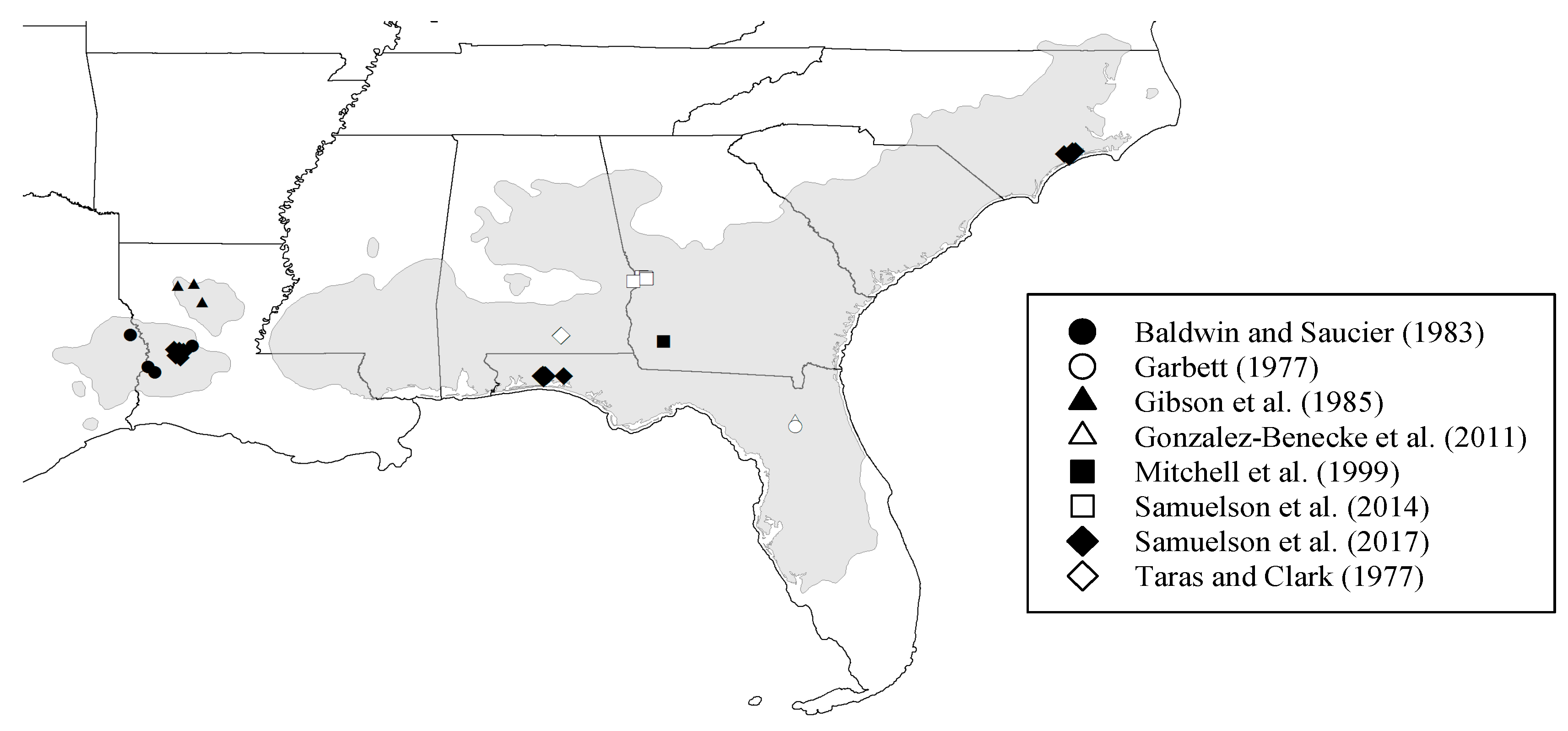
The dataset consisted of 296 longleaf pine trees measured at different sites in the southeastern U.S. The data were collected across the natural range of the species distribution (Figure 1), including trees ranging in age from 5 to 188-years-old, with DBH and HT ranging between 0.8 to 54.3 cm and 1.5 to 30.4 m, respectively (Table 2). The data were collected under different management and stand development conditions, reflecting a variety of silvicultural inputs (planting density and thinning), site characteristics (physiographic regions, soil type, and climate), origins (planted and naturally-regenerated) and developmental stage. The stand characteristics at the time of sampling were thought to cover variations in allometry due to changes in silviculture, site quality and stand age. Details on site descriptions and sampling procedure can be found in each of the publications previously mentioned. In all cases, destructive sampling was carried out. Trees were selected to include the range of sizes encountered in each study. Fresh weight of all tree components was recorded in situ. Dry mass was computed after discounting moisture content determined on subsamples of all components until reaching a constant weight. In general, foliage was oven-dried at 65–70 °C and woody tissues were oven-dried at 105 °C. For further details on biomass sampling and determination, refer to the references listed in Table 1.
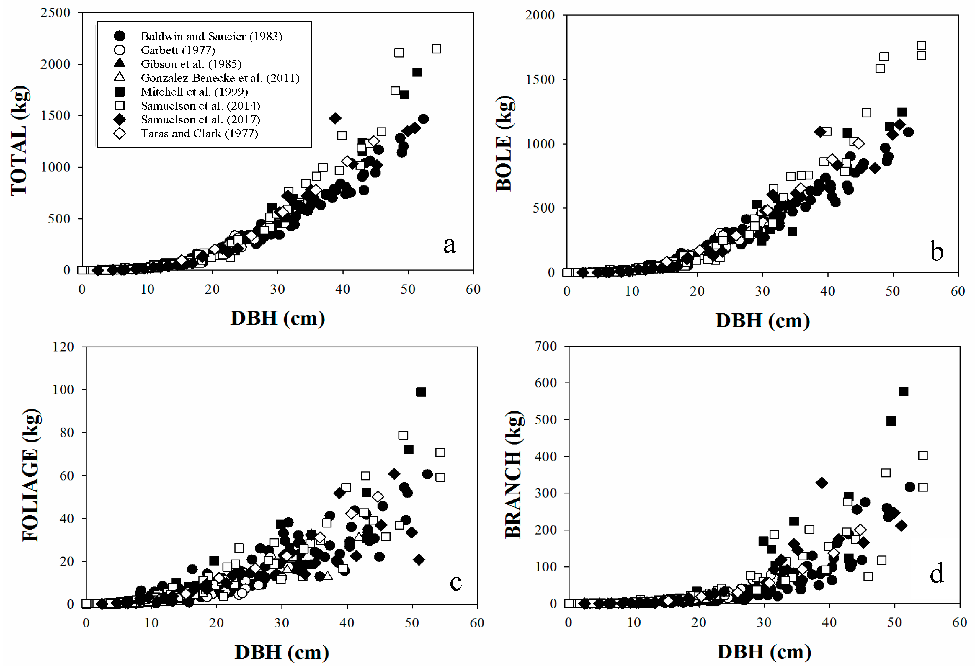
The dataset included tree-level attributes, including DBH (cm), HT (m) and dry weight of each tree above-ground component: living branches (Branch, kg); living foliage (Foliage, kg); bole outside bark (Bole, kg) and the whole-tree above-stump biomass (Total, the sum of all components in kg). The relationships between DBH and above-stump biomass components are presented in Figure 2.
With the exception of the two 188-year-old trees that were growing in isolation, the dataset included stand-level variables that characterized the plot where each selected tree was growing before being cut for biomass determination. The stand-level variables included: basal area (BA, m2 ha−1), trees per hectare (N, ha−1) and stand age (A, years). As site index (SI, m) was available for 43% of the whole dataset, that attribute was not included in the analysis. Age information for the 23 trees provided by Joseph W. Jones Ecological Research Center was not available. Due to the wide range in tree size, however, those trees were kept in the dataset and were only used for fitting local models that did not include age as covariate. Details of tree and stand characteristics of the dataset used are summarized in Table 2.
2.2. Model Specification and Estimation
Following the model structure specified in Parresol [20], the biomass models for tree bole, branch, and foliage components were constrained to equal the total tree aboveground biomass as follows:
where to represent the vector of bole, branch, foliage and total tree above-stump biomass in kg, respectively; is a nonlinear function for tree biomass component (l = 1, 2, 3 for bole, branch, and foliage, respectively); is the n × 1 vector of residuals for the ith equation (i = 1,…, 4), and n is the number of observations (trees).
Tree component biomass can be modelled as a power function of tree dimension and stand variables as:
where Xj is tree dimension and stand variables (j = 1,…, p) such as tree DBH, total tree height (HT), Age (A), stand basal area per hectare (BA), tree number per hectare (N), and , and to be estimated. Each component equation can contain its own independent variables.
Similar to Gonzalez-Benecke et al. [10], we defined six systems of equations to estimate above-stump total biomass and component biomass that depend on available predictors: (I) DBH; (II) DBH and HT; (III) DBH and A; (IV) DBH, HT and A; (V) DBH, A, N and BA; (VI) DBH, HT, A, N and BA.
The systems were fitted by the four-step fitting method [20,21] with weighted nonlinear seemingly unrelated regression (NSUR) and using the SAS/ETS® MODEL Procedure (SAS Institute Inc. 2011, Cary, NC, USA). In this estimation method, a constant 4 × 4 correlation matrix was assumed to describe the inherent correlations among biomass components and total biomass measured on the same tree; heteroscedasticity was addressed by having a unique weight function for each of the four equations. Briefly, in the first step of model estimation, all biomass components and total biomass for each model system were fitted separately with nonlinear ordinary least squares (OLS) and all significant variables were retained at α = 0.10. In the second step, for each model system, the equations of all tree components and total biomass with biomass component model forms selected in the first step were fitted by NSUR. In the third step, to model the heteroscedasticity for each equation in model (1), the estimated errors of the unweighted NSUR model from the second step were used as the dependent variable in the error variance model and fit to tree dimension variables as the form: ; the resultant significant parameter estimates form the weight function for the ith equation. In the fourth step, for each model system, the biomass components and total biomass model were refitted with NSUR after fixing the weight functions as in step 2. The resulting systems guarantee additivity in biomass equations, account for the inherent correlation among the biomass equations, and address heteroscedasticity by having a unique weighting function for each equation. Further details on the four-step NSUR fitting method can be found in Parresol [20] and Zhao et al. [21].
2.3. Model Assessment and Evaluation
Four fit statistics obtained for each system equation were employed to evaluate the goodness of fit for the biomass prediction system: mean residual (E), mean value of residuals (MABE), root mean square error (RMSE), and the coefficient of determination (R2).
In this study, the biomass equation system was fitted to the entire data set. Model validation was accomplished by the leave-one-out (LOO) cross-validation technique, in which the model system was fitted using all-but-one tree (leaving one tree out), and then the fitted model system was used to predict the values of all component and total tree biomass for that left-out tree. The summary statistics were calculated using the same Formulae (3)–(6).
2.4. Comparison Against Published Equations
The predictive performances of the new model systems were compared with the previous biomass equations reported by Baldwin and Saucier [8] and Samuelson et al. [19] using the same Formulae (3)–(6). Is important to note that the data used by these authors is already included in our dataset (Table 1). We decided to compare against these reports as they represent widely used models with the largest sampling size used for longleaf pine biomass before this publication. In both reports, D and H were used as predictors.
3. Results
3.1. Model Fitting
The six systems of biomass equations were fitted with NSUR and different weighting functions for each biomass equation. Their final model forms, in which all parameter estimates were significantly different from zero at p < 0.05, are shown as Equations (7)–(12), respectively, and the corresponding parameter estimates were presented in Table 3, Table 4, Table 5, Table 6, Table 7 and Table 8, respectively. The weighting functions and fitting statistics for each equation system are shown in Table 9.
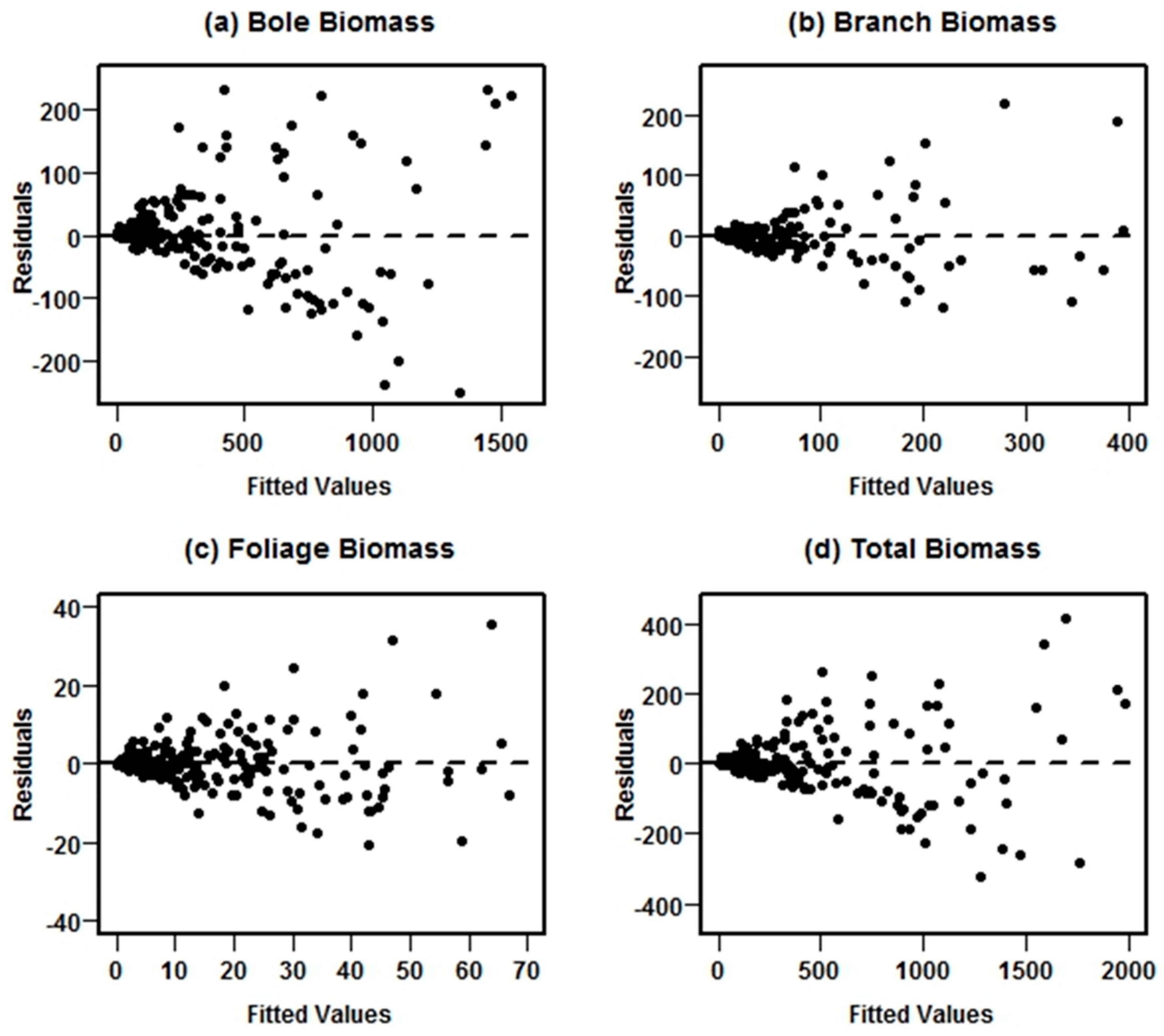
The equation systems for prediction of all biomass components and for total biomass were fitted using NSUR methods without weight functions. Scatterplots of the residuals against the predicted values for each biomass component in the unweighted equations systems revealed significant heteroscedasticity. An example of such a response for model system II is shown in Figure 3.
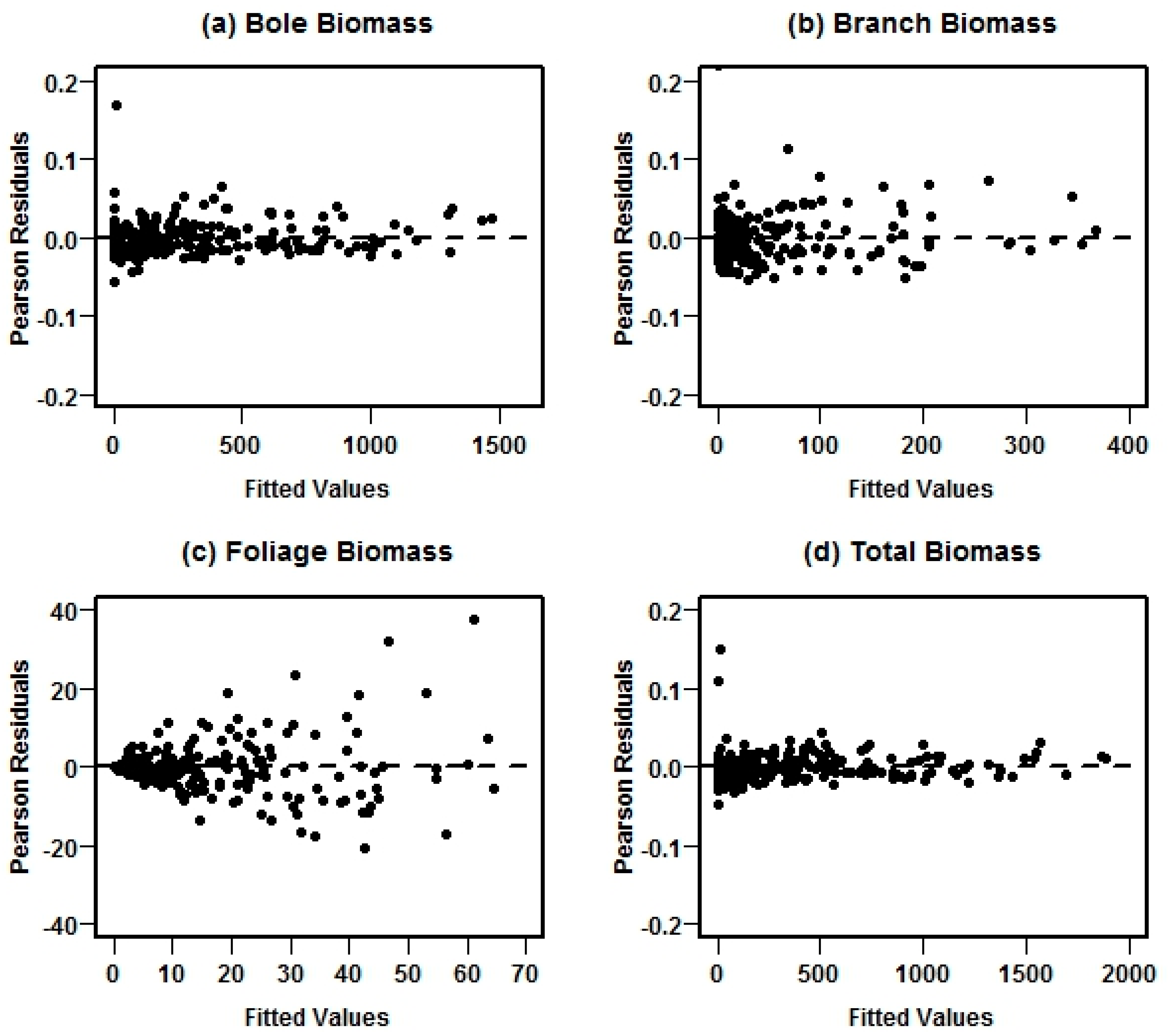
Graphical examinations suggested that, after fitting with weighting functions for each equation, there were no marked departures from homogeneous error variance and the weighted system fit the data well (Figure 4, system II as an example).
Model System I (Based on DBH)
The following equation system was fitted with NSUR and different weighting function for each biomass equation:
DBH is highly significantly in all component equations in the following DBH-based system (Table 3). The positive coefficients of DBH suggest its positive relationship with bole, branch and foliage biomass.
Model System II (based on DBH and HT)
The following equation system was fitted with NSUR and different weighting function for each biomass equation:
In the DBH and HT based system (Equation (8)), both DBH and HT are highly significant in all biomass component equations (Table 4). The positive coefficients of DBH and HT suggest their positive relationships with bole biomass. For the same DBH, the bole biomass increases with increasing tree height. However, the positive coefficient of DBH and the negative coefficient of HT in branch and foliage components imply that branch and foliage biomass increase with the increase of DBH, but for the same DBH, live branch and foliage biomass decrease with increased tree height.
Model System III (based on DBH and A)
The following equation system was fitted with NSUR and different weighting function for each biomass equation:
In the DBH and A based system (Equation (9)), DBH is significant in all component equations, but age is significant only for the bole biomass component (Table 5). This implies that with tree DBH information in the equation, the addition of tree age did not improve branch and foliage biomass estimation but did improve bole biomass estimation. The positive coefficient of A implies that for a given DBH, bole biomass increases as trees gets older. Given the same DBH, older trees usually have higher wood density than younger trees, and thus more bole biomass. The non-significant coefficient of A for branch and foliage implies that, due to crown recession, older trees do not necessarily have more (or less) crown biomass than younger trees. That lack of relationship is evident for trees older than 40 years (data not shown).
Model System IV (based on DBH, HT and A)
The following equation system was fitted with NSUR and different weighting function for each biomass equation:
For the DBH, HT and A based system (Equation (10)), however, after including both DBH and HT, tree age is significant for all component equations (Table 6). For foliage and branch biomass, the negative coefficients of HT implies that for a given DBH and A, taller trees will have lower crown biomass than smaller trees. For bole biomass, the positive coefficient of DBH, HT and A imply that bigger and older trees will have larger bole biomass.
Model System V (based on DBH, A, N and BA)
The following equation system was fitted with NSUR and different weighting functions for each biomass equation:
After including tree DBH and stand basal area (BA) in this system (Equation (11)), tree age (A) and trees per ha (N) are still significant in the bole and foliage biomass equations (Table 7). For branch biomass N and A are not significant, implying that when DBH and BA are known, N and A are not necessary to estimate branch biomass. For branch and foliage, the negative coefficient of BA implies that for a given DBH and A, trees growing in stands with higher stocking will have lower crown biomass than trees growing in less stocked stands.
Model System VI (based on DBH, HT, A, N and BA)
The following equation system was fitted with NSUR and different weighting function for each biomass equation:
The only difference between this system (Equation (12)) and the system IV (Equation (10)) is associated with the branch biomass equation. In addition to DBH and HT, the branch biomass equation included BA in system VI, instead of including A in the system IV. When A or BA, together with DBH and HT are included in that system, N was not necessary (N is non-significant) for any component of above-stump biomass (Table 8). For bole biomass, the positive coefficient of DBH, HT and A implies that bigger and older trees will have larger bole biomass. For branch biomass, the negative coefficient of HT and BA implies that for a given DBH and BA, taller trees will have lower branch biomass than smaller trees, and for a given DBH and HT, trees growing in more stocked stands will have lower crown biomass than trees growing in less stocked stands. For foliage biomass, the negative coefficient of HT implies that for a given DBH and A, taller trees will have lower crown biomass than smaller trees.
Compared to the system I (based on DBH only), system II including additional HT or the system III including additional tree age improves the prediction of all component biomass and total biomass (Table 9), and system III was better (higher R2, and lower E, MABE and RMSE). With the inclusion of DBH and HT, including tree age information in systems IV or VI further improved the prediction of all component biomass and total biomass. There are no large differences in biomass estimation between systems IV and VI. That is, when tree DBH, HT and A information are available, system IV could be enough, and BA information is not needed for system VI. Including stand density information (BA and N), although without tree height, system V improves the prediction of branch and foliage biomass.
There were not any obvious trends in the plots of biomass residuals against A, N, or BA. An example of residual plots against A and BA for Model VI is presented as supplementary material (Figure S1).
3.2. Model Validation
The leave-one-out (LOO) cross-validation statistics indicated that all systems showed high accuracy, with no clear trend of bias on biomass estimations (Table 10). The mean residuals ranged between −3.29 to 3.38 (−1.2%–1.2%) for bole, −0.77 to 1.79 (−1.6%–3.8%) for branch, −0.36 to 0.04 (−2.7%–0.3%) for foliage and −3.19 to 4.9 (−1.0%–1.5%) for total biomass. Compared with the model system I (only DBH as predictor), including DBH and HT in the model system II improved the precision of the estimations, reducing RMSE from 34, 79.6, 48.5 and 29.1% to 25.2, 73.4, 47.8 and 26.2% of mean observed value, for bole, branch, foliage and total biomass, respectively (Table 10). When DBH and A were incorporated into the model (Model system III), further improvement in the precision of the estimations was observed, reducing RMSE to 22.7, 57.1, 42.9 and 19.6%, for bole, branch, foliage and total biomass, respectively. When DBH, HT and A were included into the model (model system IV) even larger reductions in RMSE were observed for bole (14.6%), branch (53.0%) and total (16.0%) biomass, but not for foliage biomass (42.9%) (Table 10). The inclusion of N and/or BA (model systems V and VI) showed no improvement in the precision of any biomass estimations.
3.3. Comparison against Published Equations
Model prediction statistics for the models reported by Baldwin and Saucier [7] (BS-83) and Samuelson et al. [17] (S-17) are shown in Table 11. Even though the coefficient of determination of bole and total biomass was larger than 0.93, the precision and accuracy of both reported models were lower than the models reported in this study. For example, when compared with model system II, the RMSE was increased from 25.2, 73.4, 47.8 and 26.2% on model system II, to 28.8, 98.5, 55.6 and 30.2%, on BS-83, or 31.4, 78.7, 50.9 and 31.6%, on S-17, for bole, branch, foliage and total biomass, respectively (compare Table 10 and Table 11). Interestingly, the model S-17 showed a tendency of overestimating on about 11% all biomass components.
Graphical analysis of the actual biomass and that predicted by the equations reported by Baldwin and Saucier [8] (BS-83) and Samuelson et al. [19] (S-17), and new equation systems developed in this study indicate that the new equation systems predicted all biomass components on the larger dataset with great precision and accuracy. In Figure 5 we show the results for model system II and VI. The estimates of all biomass components were highly improved with equation system VI.
4. Discussion
General and local additive models are useful to determine bole, living branches, foliage and total above-ground tree components. The additive models used in this study ensure that total biomass will be equal to the sum of the parts. Depending on data availability and level of accuracy desired, the users should decide which model to apply.
The set of biomass equations were developed using data from trees growing on sites distributed over the range of the species distribution across the southeastern U.S., spanning a wide range of ages and stand characteristics. This comprehensive data analysis provides confidence that the biomass functions reported here can be used over a broad range of stand development and management conditions. As thinning may affect stand structure, and we do not have records of years since thinning on the sampled trees, we recommend using our general models with caution on conditions soon after thinning.
Similar to Zhao et al. [21] and Poudel and Temesgen [22], in this study we used the biomass additivity approach, which guarantees that total above-ground biomass will be equal to the sum of the parts (bole, living branches and foliage). As Parresol [20] concluded, biomass additivity is a preferred attribute of a biomass equations system. All previous biomass equations reported for longleaf pine including the biomass equations of Baldwin and Saucier [8] and Samuelson et al. [19] used in this study for comparison are not additive, as they were fitted separately for each component and total biomass. This model structure was used to ensure the additivity property of nonlinear models. The four-step fitting approach used in this study improved model estimation, increasing accuracy and precision of biomass predictions. Furthermore, the estimated weighting function eliminated heteroscedasticity for each of the biomass functions.
The models that estimated foliage biomass showed little improvement when HT (model system II) and/or tree age were included. Similar response was observed by Gonzalez-Benecke et al. [10] for Pinus taeda L. and P. elliottii Engelm. trees. Compared with system I (based on DBH only), system III additionally included tree age which was significant only in the bole biomass equation, but also improved the branch and total biomass predictions. This response may be related to changes in wood density as trees age [9,22] and the interdependence of additive models. When A was included in the models that used DBH and HT (model system IV), it was significant in bole, branch and foliage equations, improving bole, branch and total biomass predictions. Although BA, rather than A, was significant in the branch biomass equation in system VI, that system did not predict component and total biomass better than system IV. When BA was significant in model systems V and VI, the parameter estimate for BA for foliage and branch was always negative, implying that for the same stem size and age, trees growing in stands with more intraspecific competition had smaller crown biomass than trees growing in stands with less intraspecific competition.
Even though the functions reported in this study can be used to estimate above-ground biomass directly, these equations have potential use in a variety of management and ecological applications. Several forest ecologists have used allometric biomass equations to quantify processes in forest ecosystems, such as nutrient dynamics, carbon sequestration, growth and competition (e.g., [10,23,24,25,26,27]), and better biomass predictions would find practical applications in nascent carbon-trading markets [28]. Our new biomass equations should improve these types of analyses in longleaf pine forest ecosystems. Process-based models, such as 3-PG [29] will also benefit from these more accurate and adaptable functions. Modeling systems that incorporate these equations can also be used to explore the effects of variable tree-level allometry on stand dynamics [30].
All previously reported, biomass functions for longleaf pine trees rely on DBH only [7,15,19] or DBH and HT [8,9,15,16,17,19]. When compared with our model system VI, the functions of Baldwin and Saucier [8] and Samuelson et al. [19] showed a tendency to estimate biased results. In addition to more accurate estimations, our models provide the additivity property to the biomass determinations.
5. Conclusions
The equations to estimate above-ground biomass for longleaf pine trees reported in this study offer valuable tools for the study and management of the species. Our new systems of biomass equations are the first reported for longleaf pine that include age and stand attributes such as N and BA, all easily available in regular inventories or with growth and yield models [31]. The equations presented in this study allow robust estimates of biomass components using easily available stand attributes as covariates, and at the same time, ensuring biomass component additivity.
Supplementary Materials
The following are available online at https://www.mdpi.com/1999-4907/9/6/310/s1, Figure S1: Pearson residual plots against age (left panel) and Basal Area (BA, right panel) for each biomass component in the model system VI fitted using NSUR method. There were not any obvious trends in the plots of biomass residuals against Age or BA.
Author Contributions
L.J.S., T.A.M. S.B.J. and D.J.L. shared datasets and edited the manuscript, D.Z. and C.A.G.B. analyzed the data and wrote the paper.
Acknowledgments
This research was supported by the U.S. Department of Defense, through the Strategic Environmental Research and Development Program (SERDP), the University of Florida’s Carbon Resources Science Center, the Forest Biology Research Cooperative, the USDA National Institute of Food and Agriculture, Coordinated Agricultural Project Award #2011-68002-30185, and the USDA Forest Service (Agreement 16-JV-11330145-075). The authors acknowledge, with thanks to Tom Stokes, all individuals who contributed to collecting the biomass data used in this study.
Conflicts of Interest
The authors declare no conflict of interest and the founding sponsors had no role in the design of the study; in the collection, analyses, or interpretation of data; in the writing of the manuscript, and in the decision to publish the results.
References
- Madgwick, H.; Satoo, T. On estimating the aboveground weights of tree stands. Ecology 1975, 56, 1446–1450. [Google Scholar] [CrossRef]
- Jenkins, J.C.; Chojnacky, D.C.; Heath, L.S.; Birdsey, R.A. National-scale biomass estimators for United States tree species. For. Sci. 2003, 49, 12–35. [Google Scholar]
- Johansen, R.W.; McNab, W.H. Estimating logging residue weights from standing slash pine for prescribed burns. South. J. Appl. For. 1977, 1, 2–6. [Google Scholar]
- Hepp, T.D.; Brister, G.H. Estimating crown biomass in loblolly pine plantations in the Carolina flatwoods. For. Sci. 1982, 28, 115–127. [Google Scholar]
- Johnsen, K.H.; Keyser, T.; Butnor, J.R.; Gonzalez-Benecke, C.A.; Kaczmarek, D.J.; Maier, C.A.; McCarthy, H.R.; Sun, G. Forest productivity and carbon sequestration of forests in the southern United States. In Climate Change Adaptation and Mitigation Management Options: A Guide for Natural Resource Managers in Southern Forest Ecosystems; Vose, J.M., Klepzig, K.D., Eds.; CRC Press: Boca Raton, FL, USA, 2014; pp. 193–247. [Google Scholar]
- Marziliano, P.A.; Coletta, V.; Menguzzato, G.; Nicolaci, A.; Pellicone, G.; Veltri, A. Effects of planting density on the distribution of biomass in a douglas-fir plantation in southern Italy. iForest 2015, 8, 368–376. [Google Scholar] [CrossRef] [Green Version]
- Mitchell, R.J.; Kirkman, L.K.; Pecot, S.D.; Wilson, C.A.; Palik, B.J.; Boring, L.R. Patterns and controls of ecosystem function in longleaf pine–wiregrass savannas. I. Aboveground net primary productivity. Can. J. For. Res. 1999, 29, 743–751. [Google Scholar] [CrossRef]
- Baldwin, V.C., Jr.; Saucier, J.R. Aboveground Weight and Volume of Unthinned, Planted Longleaf Pine on West Gulf Forest Sites; Research Paper SO-191; U.S. Department of Agriculture, Forest Service, Southern Forest Experiment Station: New Orleans, LA, USA, 1983; 25p.
- Samuelson, L.J.; Stokes, T.A.; Butnor, J.R.; Johnsen, K.H.; Gonzalez-Benecke, C.A.; Anderson, P.H.; Jackson, J.; Ferrari, L.; Martin, T.A.; Cropper, W.P., Jr. Ecosystem carbon stocks in Pinus palustris forests. Can. J. For. Res. 2014, 44, 476–486. [Google Scholar] [CrossRef]
- Gonzalez-Benecke, C.A.; Gezan, S.A.; Albaugh, T.J.; Allen, H.L.; Burkhart, H.E.; Fox, T.R.; Jokela, E.J.; Maier, C.A.; Martin, T.A.; Rubilar, R.A.; et al. Local and general above-stump biomass functions for loblolly and slash pine trees. For. Ecol. Manag. 2014, 334, 254–276. [Google Scholar] [CrossRef]
- Kralicek, K.; Huy, B.; Poudel, K.P.; Temesgen, H.; Salas, C. Simultaneous estimation of above- and below-ground biomass in tropical forests of Viet Nam. For. Ecol. Manag. 2014, 390, 147–156. [Google Scholar] [CrossRef]
- Forrester, D.I.; Tachauer, I.H.H.; Annighoefer, P.; Barbeito, I.; Pretzsch, H.; Ruiz-Peinado, R.; Stark, H.; Cacchiano, G.; Zlatanov, T.; Chakraborty, T.; et al. Generalized biomass and leaf area allometric equations for European tree species incorporating stand structure, tree age and climate. For. Ecol. Manag. 2017, 396, 160–175. [Google Scholar] [CrossRef]
- Frost, C.C. History and future of the longleaf pine ecosystem. In The Longleaf Pine Ecosystem—Ecology, Silviculture and Restoration; Jose, S., Jokela, E.J., Miller, D.L., Eds.; Springer: New York, NY, USA, 2006; pp. 9–48. [Google Scholar]
- Brockway, D.G.; Outcalt, K.W.; Tomczak, D.J.; Johnson, E.E. Restoration of Longleaf Pine Ecosystems; General Technical Report SRS-83; U.S. Department of Agriculture, Forest Service, Southern Research Station: Asheville, NC, USA, 2005; p. 34. [Google Scholar]
- Garbett, W.S. Aboveground Biomass and Nutrient Content of a Mixed Slash-Longleaf Pine Stand in Florida. Master’s Thesis, University of Florida, Gainesville, FL, USA, 1977. [Google Scholar]
- Taras, M.A.; Clark, A., III. Aboveground Biomass of Longleaf Pine in a Natural Sawtimber Stand in Southern Alabama; USDA Forest Service Research Paper SE 162; Department of Agriculture, Forest Service, Southeastern Forest Experiment Station: Asheville, NC, USA, 1977; p. 32.
- Gibson, M.D.; McMillin, C.W.; Shoulders, E. Above- and Below-Ground Biomass of Four Species of Southern Pine Growing on Three Sites in Louisiana; USDA Forest Service Final Report FS-SO-3201-59; USDA, Forest Service, Southern Forest Experiment Station: Pineville, LA, USA, 1985.
- Gonzalez-Benecke, C.A.; Martin, T.A.; Cropper, W.P., Jr. Whole-tree water relations of co-occurring mature Pinus palustris and Pinus elliottii. Can. J. For. Res. 2011, 41, 509–523. [Google Scholar] [CrossRef]
- Samuelson, L.J.; Stokes, T.A.; Butnor, J.R.; Johnsen, K.H.; Gonzalez-Benecke, C.A.; Martin, T.A.; Cropper, W.P., Jr.; Anderson, P.H.; Ramirez, M.; Lewis, J. Ecosystem carbon density and allocation across a chronosequence of longleaf pine forests in the southeastern USA. Ecol. Appl. 2017, 27, 244–259. [Google Scholar] [CrossRef] [PubMed]
- Parresol, B.R. Additivity of nonlinear biomass equations. Can. J. For. Res. 2001, 31, 865–878. [Google Scholar] [CrossRef]
- Zhao, D.; Kane, M.; Markewitz, D.; Teskey, R.; Clutter, M. Additive tree biomass equations for midrotation loblolly pine plantations. For. Sci. 2015, 61, 613–623. [Google Scholar] [CrossRef]
- Poudel, K.P.; Temesgen, H. Developing biomass equations for Western hemlock and red alder trees in Western Oregon forests. Forests 2016, 7, 88. [Google Scholar] [CrossRef]
- Larson, P.R.; Kretschmann, D.E.; Clark, A., III; Isen-brands, J.G. Juvenile Wood Formation and Proper-Ties in Southern Pine; General Technical Report FPL-GTR-129; U.S. Department of Agriculture, Forest Service, Forest Products Laboratory: Madison, WI, USA, 2001. [Google Scholar]
- Gholz, H.L.; Fisher, R.F. Organic matter production and distribution in slash pine (Pinus elliottii) plantations. Ecology 1982, 63, 1827–1839. [Google Scholar] [CrossRef]
- Gholz, H.L.; Fisher, R.F.; Pritchett, W.L. Nutrient Dynamics in Slash Pine Plantation Ecosystems. Ecology 1985, 66, 647–659. [Google Scholar] [CrossRef]
- Waring, R.H.; Landsberg, J.J.; Williams, M. Net primary production of forests: A constant fraction of gross primary production? Tree Physiol. 1998, 18, 129–134. [Google Scholar] [CrossRef] [PubMed]
- Vogel, J.G.; Suau, L.J.; Martin, T.A.; Jokela, E.J. Long-term effects of weed control and fertilization on the carbon and nitrogen pools of a slash and loblolly pine forest in north-central Florida. Can. J. For. Res. 2011, 41, 552–567. [Google Scholar] [CrossRef]
- Berndes, G.; Abt, B.; Asikainen, A.; Cowie, A.; Dale, V.; Egnell, G.; Lindner, M.; Marelli, L.; Paré, D.; Pingoud, K.; et al. Forest Biomass, Carbon Neutrality and Climate Change Mitigation; From Science to Policy 3; European Forest Institute: Joensuu, Finland, 2016; p. 27. [Google Scholar]
- Landsberg, J.J.; Waring, R.H. A generalized model of forests productivity using simplified concepts of radiation-use efficiency, carbon balance and partitioning. For. Ecol. Manag. 1997, 95, 209–228. [Google Scholar] [CrossRef]
- Gonzalez-Benecke, C.A.; Samuelson, L.J.; Martin, T.A.; Cropper, W.P., Jr.; Stokes, T.A.; Butnor, J.R.; Johnsen, K.H.; Anderson, P.H. Modeling the effects of forest management on in situ and ex situ longleaf pine forest carbon stocks. For. Ecol. Manag. 2015, 355, 24–36. [Google Scholar] [CrossRef] [Green Version]
- Gonzalez-Benecke, C.A.; Gezan, S.A.; Leduc, D.J.; Martin, T.A.; Cropper, W.P., Jr.; Samuelson, L.J. Modeling survival, yield, volume partitioning and their response to thinning for longleaf pine (Pinus palustris Mill.) plantations. Forests 2015, 3, 1104–1132. [Google Scholar] [CrossRef]
Figure 1.
Location of the study sites for longleaf pine within the species natural distribution range (grey area).
Figure 1.
Location of the study sites for longleaf pine within the species natural distribution range (grey area).

Figure 2.
Relationship between DBH and (a) total tree above-stump biomass (TOTAL, kg); (b) bole biomass outside bark (BOLE, kg); (c) living foliage biomass (FOLIAGE, kg); and (d) living branch biomass outside bark (BRANCH, kg) for longleaf pine trees used in this study.
Figure 2.
Relationship between DBH and (a) total tree above-stump biomass (TOTAL, kg); (b) bole biomass outside bark (BOLE, kg); (c) living foliage biomass (FOLIAGE, kg); and (d) living branch biomass outside bark (BRANCH, kg) for longleaf pine trees used in this study.

Figure 3.
Residual plots for each biomass component in the model system II fitted using NSUR without weight function, showing significant heteroscedasticity.
Figure 3.
Residual plots for each biomass component in the model system II fitted using NSUR without weight function, showing significant heteroscedasticity.

Figure 4.
Pearson residual plots for each biomass component in the model system II fitted using NSUR method and different weight functions for each system equation with its own weight function.
Figure 4.
Pearson residual plots for each biomass component in the model system II fitted using NSUR method and different weight functions for each system equation with its own weight function.

Figure 5.
Comparison of each component and total biomass with the model systems II (NM-2) and VI (NM-6), and previously published biomass equations of Baldwin and Saucier [8] (BS-83) and Samuelson et al. [19] (S-17).


Table 1.
Summary biomass measurement per institution.
| Institution | n | A (years) | Stand Type | Thinning | Reference |
|---|---|---|---|---|---|
| Auburn University | 32 | 5–87 | Planted/Natural | Yes (if age >21 years) | Samuelson et al. (2014) |
| 96 | 8–188 | Planted/Natural | Yes (if age >25 years) | Samuelson et al. (2017) | |
| Joseph W. Jones Ecological Research Center | 23 | 19–166 | Planted/Natural | Yes | Mitchell et al. (1999) |
| University of Florida | 12 | 36–56 | Natural | Yes | Garbett (1977) |
| 4 | 70 | Natural | Yes | Gonzalez-Benecke et al. (2011) | |
| U.S. Forest Service | 7 | 34–64 | Natural | Yes | Taras and Clark (1977) |
| 111 | 10–44 | Planted | No | Baldwin and Saucier (1983) | |
| 11 | 25 | Planted | No | Gibson et al. (1985) |
n: number of sampled trees; A: range of age of measured trees (years).
Table 2.
Summary statistics of tree and their associated stand characteristics for the sampled longleaf pine trees.
Table 2.
Summary statistics of tree and their associated stand characteristics for the sampled longleaf pine trees.
| Attribute | Unit | n | Mean | Std Dev | Minimum | Maximum |
|---|---|---|---|---|---|---|
| A | year | 273 | 35.4 | 25.6 | 5 | 188 |
| DBH | cm | 296 | 21.4 | 13.4 | 0.8 | 54.3 |
| HT | m | 296 | 15.8 | 7.4 | 1.5 | 30.4 |
| N | ha−1 | 296 | 991 | 766 | 50 | 2750 |
| BA | m2 ha−1 | 296 | 22.6 | 14.3 | 0.3 | 52.0 |
| Branch | kg | 291 | 47.7 | 83.2 | 0.0 | 576.9 |
| Foliage | kg | 296 | 13.6 | 15.8 | 0.0 | 99.0 |
| Bole | kg | 292 | 271.2 | 344.8 | 0.3 | 1762.4 |
| Total | kg | 291 | 330.4 | 431.0 | 0.6 | 2149.9 |
A: tree/stand age (years); DBH: diameter outside-bark at 1.37 m height (cm); HT: total tree height (m); N: trees per hectare (ha−1); BA: stand basal area (m2 ha−1); Branch: total living branch biomass (kg); Foliage: total living needles biomass (kg); Bole: above-stump stem over bark biomass (kg); Total: total above-stump biomass (kg).
Table 3.
Parameter estimates and their asymptotic standard error and p-values for the additive biomass equation system based on diameter at breast height (DBH) only (Model System I).
Table 3.
Parameter estimates and their asymptotic standard error and p-values for the additive biomass equation system based on diameter at breast height (DBH) only (Model System I).
| Biomass Component | Variable | Parameter | Asymptotic Estimate | Standard Error | p-Value |
|---|---|---|---|---|---|
| Bole | 0.0725 | 0.0079 | <0.0001 | ||
| DBH | 2.5074 | 0.0317 | <0.0001 | ||
| Branch | 0.0016 | 0.0002 | <0.0001 | ||
| DBH | 3.0786 | 0.0387 | <0.0001 | ||
| Foliage | 0.0214 | 0.0051 | <0.0001 | ||
| DBH | 2.0051 | 0.0640 | <0.0001 |
Table 4.
Parameter estimates and their asymptotic standard error and p-values for the additive biomass equation system based on diameter at breast height (DBH) and height (HT) (Model System II).
Table 4.
Parameter estimates and their asymptotic standard error and p-values for the additive biomass equation system based on diameter at breast height (DBH) and height (HT) (Model System II).
| Biomass Component | Variable | Parameter | Asymptotic Estimate | Standard Error | p-Value |
|---|---|---|---|---|---|
| Bole | 0.0273 | 0.0027 | <0.0001 | ||
| DBH | 1.9745 | 0.0409 | <0.0001 | ||
| HT | 0.9163 | 0.0618 | <0.0001 | ||
| Branch | 0.0070 | 0.0021 | <0.0001 | ||
| DBH | 3.6735 | 0.1268 | <0.0001 | ||
| HT | −1.1735 | 0.1857 | <0.0001 | ||
| Foliage | 0.0697 | 0.0153 | <0.0001 | ||
| DBH | 2.1631 | 0.0908 | <0.0001 | ||
| HT | −0.5569 | 0.1250 | <0.0001 |
Table 5.
Parameter estimates and their asymptotic standard error and p-values for the additive biomass equation system based on diameter at breast height (DBH) and age (A) (Model System III).
Table 5.
Parameter estimates and their asymptotic standard error and p-values for the additive biomass equation system based on diameter at breast height (DBH) and age (A) (Model System III).
| Biomass Component | Variable | Parameter | Asymptotic Estimate | Standard Error | p-Value |
|---|---|---|---|---|---|
| Bole | 0.0531 | 0.0061 | <0.0001 | ||
| DBH | 2.1674 | 0.0398 | <0.0001 | ||
| A | 0.4012 | 0.0338 | <0.0001 | ||
| Branch | 0.0019 | 0.0003 | <0.0001 | ||
| DBH | 3.0045 | 0.0395 | <0.0001 | ||
| Foliage | 0.0259 | 0.0065 | <0.0001 | ||
| DBH | 1.9399 | 0.0683 | <0.0001 |
Table 6.
Parameter estimates and their asymptotic standard error and p-values for the additive biomass equation system based on diameter at breast height (DBH), height (HT) and age (A) (Model System IV).
Table 6.
Parameter estimates and their asymptotic standard error and p-values for the additive biomass equation system based on diameter at breast height (DBH), height (HT) and age (A) (Model System IV).
| Biomass Component | Variable | Parameter | Asymptotic Estimate | Standard Error | p-Value |
|---|---|---|---|---|---|
| Bole | 0.0155 | 0.0013 | <0.0001 | ||
| DBH | 1.8026 | 0.0370 | <0.0001 | ||
| HT | 0.9220 | 0.0518 | <0.0001 | ||
| A | 0.3068 | 0.0261 | <0.0001 | ||
| Branch | 0.0027 | 0.0006 | <0.0001 | ||
| DBH | 3.4396 | 0.1082 | <0.0001 | ||
| HT | −0.9013 | 0.1549 | <0.0001 | ||
| A | 0.2413 | 0.0796 | 0.0027 | ||
| Foliage | 0.0504 | 0.0060 | <0.0001 | ||
| DBH | 1.8671 | 0.0910 | <0.0001 | ||
| HT | −0.3543 | 0.1070 | 0.0011 | ||
| A | 0.1894 | 0.0538 | 0.0005 |
Table 7.
Parameter estimates and their asymptotic standard error and p-values for the additive biomass equation system based on diameter at breast height (DBH), age (A), number of trees per hectare (N) and basal area (BA) (Model System V).
Table 7.
Parameter estimates and their asymptotic standard error and p-values for the additive biomass equation system based on diameter at breast height (DBH), age (A), number of trees per hectare (N) and basal area (BA) (Model System V).
| Biomass Component | Variable | Parameter | Asymptotic Estimate | Standard Error | p-Value |
|---|---|---|---|---|---|
| Bole | 0.0597 | 0.0167 | 0.0004 | ||
| DBH | 2.1131 | 0.0369 | <0.0001 | ||
| A | 0.4143 | 0.0468 | <0.0001 | ||
| N | −0.0672 | 0.0276 | 0.0158 | ||
| BA | 0.1436 | 0.0326 | <0.0001 | ||
| Branch | 0.0034 | 0.0004 | <0.0001 | ||
| DBH | 2.9823 | 0.0454 | <0.0001 | ||
| BA | −0.1638 | 0.0386 | <0.0001 | ||
| Foliage | 0.0061 | 0.0039 | 0.1196 | ||
| DBH | 1.9523 | 0.0968 | <0.0001 | ||
| A | 0.2825 | 0.1134 | 0.0134 | ||
| N | 0.1673 | 0.0669 | 0.0131 | ||
| BA | −0.2193 | 0.0946 | 0.0213 |
Table 8.
Parameter estimates and their asymptotic standard error and p-values for the additive biomass equation system based on diameter at breast height (DBH), height (HT), age (A) and basal area (BA) (Model System VI).
Table 8.
Parameter estimates and their asymptotic standard error and p-values for the additive biomass equation system based on diameter at breast height (DBH), height (HT), age (A) and basal area (BA) (Model System VI).
| Biomass Component | Variable | Parameter | Asymptotic Estimate | Standard Error | p-Value |
|---|---|---|---|---|---|
| Bole | 0.0156 | 0.0013 | <0.0001 | ||
| DBH | 1.7983 | 0.0364 | <0.0001 | ||
| HT | 0.9285 | 0.0509 | <0.0001 | ||
| A | 0.3031 | 0.0249 | <0.0001 | ||
| Branch | 0.0042 | 0.0009 | <0.0001 | ||
| DBH | 3.4396 | 0.1122 | <0.0001 | ||
| HT | −0.5562 | 0.1565 | 0.0005 | ||
| BA | −0.1958 | 0.0475 | 0.0001 | ||
| Foliage | 0.0420 | 0.0065 | <0.0001 | ||
| DBH | 1.8393 | 0.0939 | <0.0001 | ||
| HT | −0.2730 | 0.1129 | 0.0164 | ||
| A | 0.1956 | 0.0549 | 0.0004 |
Table 9.
Weight functions and fit statistics for each component in the additive biomass equation systems.
Table 9.
Weight functions and fit statistics for each component in the additive biomass equation systems.
| Model System | Biomass Component | Weight Function | E | MABE | RMSE | R2 |
|---|---|---|---|---|---|---|
| I | Bole | −0.714 | 47.760 | 90.496 | 0.929 | |
| Branch | −0.754 | 16.656 | 37.130 | 0.797 | ||
| Foliage | 0.036 | 3.823 | 6.446 | 0.838 | ||
| Total | −1.431 | 48.366 | 94.403 | 0.951 | ||
| II | Bole | 3.281 | 34.649 | 67.064 | 0.961 | |
| Branch | 1.730 | 14.736 | 34.058 | 0.830 | ||
| Foliage | −0.300 | 3.685 | 6.250 | 0.847 | ||
| Total | 4.711 | 43.950 | 84.532 | 0.961 | ||
| III | Bole | −0.008 | 33.517 | 59.469 | 0.969 | |
| Branch | 0.402 | 13.004 | 26.741 | 0.850 | ||
| Foliage | 0.017 | 3.550 | 5.720 | 0.850 | ||
| Total | 0.412 | 33.721 | 62.646 | 0.977 | ||
| IV | Bole | −0.080 | 21.839 | 38.223 | 0.987 | |
| Branch | −0.732 | 11.252 | 24.582 | 0.873 | ||
| Foliage | −0.376 | 3.557 | 5.635 | 0.854 | ||
| Total | −1.189 | 28.440 | 51.307 | 0.984 | ||
| V | Bole | −3.519 | 33.002 | 59.264 | 0.969 | |
| Branch | 0.032 | 12.599 | 26.113 | 0.857 | ||
| Foliage | 0.036 | 3.404 | 5.565 | 0.858 | ||
| Total | −3.452 | 33.791 | 62.196 | 0.977 | ||
| VI | Bole | 0.485 | 21.841 | 38.402 | 0.987 | |
| Branch | −0.330 | 11.306 | 24.602 | 0.873 | ||
| Foliage | −0.298 | 3.560 | 5.641 | 0.854 | ||
| Total | −0.143 | 28.006 | 50.856 | 0.985 |
E is mean residual; MABE is mean value of residuals; RMSE is root mean square error; R2 is the coefficient of determination.
Table 10.
Leave-one-out (LOO) cross-validation results for each biomass component in the additive biomass equation systems.
Table 10.
Leave-one-out (LOO) cross-validation results for each biomass component in the additive biomass equation systems.
| Model System | Biomass Component | E | MABE | RMSE | R2 |
|---|---|---|---|---|---|
| I | Bole | −0.85 (−0.3) | 48.42 (17.9) | 92.21 (34.0) | 0.927 |
| Branch | −0.72 (−1.5) | 16.89 (35.4) | 37.97 (79.6) | 0.788 | |
| Foliage | 0.04 (0.3) | 3.88 (28.5) | 6.60 (48.5) | 0.830 | |
| Total | −1.52 (−0.5) | 49.05 (14.8) | 96.23 (29.1) | 0.949 | |
| II | Bole | 3.38 (1.2) | 35.17 (13.0) | 68.30 (25.2) | 0.960 |
| Branch | 1.79 (3.8) | 15.01 (31.5) | 34.99 (73.4) | 0.820 | |
| Foliage | −0.29 (−2.1) | 3.77 (27.7) | 6.50 (47.8) | 0.835 | |
| Total | 4.88 (1.5) | 44.72 (13.5) | 86.54 (26.2) | 0.959 | |
| III | Bole | −0.09 (0.0) | 34.42 (12.7) | 61.54 (22.7) | 0.966 |
| Branch | 0.48 (−1.0) | 13.24 (27.7) | 27.25 (57.1) | 0.844 | |
| Foliage | 0.03 (0.3) | 3.62 (26.6) | 5.84 (42.9) | 0.843 | |
| Total | 0.42 (0.1) | 34.55 (10.5) | 64.77 (19.6) | 0.975 | |
| IV | Bole | 0.05 (0.0) | 22.46 (8.3) | 39.50 (14.6) | 0.986 |
| Branch | −0.77 (−1.6) | 11.54 (24.2) | 25.29 (53.0) | 0.866 | |
| Foliage | −0.36 (−2.7) | 3.65 (26.8) | 5.84 (42.9) | 0.844 | |
| Total | −1.08 (−0.3) | 29.18 (8.8) | 52.94 (16.0) | 0.983 | |
| V | Bole | −3.29 (−1.2) | 34.97 (12.9) | 63.97 (23.6) | 0.964 |
| Branch | 0.05 (0.1) | 12.79 (26.8) | 26.66 (55.9) | 0.851 | |
| Foliage | 0.04 (0.3) | 3.56 (26.2) | 5.95 (43.8) | 0.837 | |
| Total | −3.19 (−1.0) | 35.79 (10.8) | 66.27 (20.1) | 0.974 | |
| VI | Bole | 0.64 (0.2) | 22.48 (8.3) | 39.76 (14.7) | 0.986 |
| Branch | −0.32 (−0.7) | 11.59 (24.3) | 25.29 (53.0) | 0.866 | |
| Foliage | −0.28 (−2.1) | 3.66 (26.9) | 5.85 (43.0) | 0.843 | |
| Total | 0.04 (0.0) | 28.72 (8.7) | 52.43 (15.9) | 0.984 |
E is mean residual; MABE is mean value of residuals; RMSE is root mean square error; R2 is the coefficient of determination. Values in parenthesis corresponds to percent relative to mean observed value.
Table 11.
Prediction statistics for each component using biomass equations developed by Baldwin and Saucier (1983) and Samuelson et al. (2017).
Table 11.
Prediction statistics for each component using biomass equations developed by Baldwin and Saucier (1983) and Samuelson et al. (2017).
| Model System | Component | E | MABE | RMSE | R2 |
|---|---|---|---|---|---|
| Baldwin and Saucier (1983) (BS-83) | Bole | 25.19 (9.3) | 35.96 (13.3) | 78.15 (28.8) | 0.947 |
| Branch | −2.63 (−5.5) | 23.77 (49.8) | 47.01 (98.5) | 0.675 | |
| Foliage | 0.99 (7.2) | 4.54 (33.3) | 7.59 (55.6) | 0.775 | |
| Total | 27.85 (8.4) | 46.32 (14.0) | 99.75 (30.2) | 0.945 | |
| Samuelson et al. (2017) (S-17) | Bole | −28.87 (−10.6) | 43.53 (16.1) | 85.14 (31.4) | 0.937 |
| Branch | −5.22 (−10.9) | 17.96 (37.6) | 37.55 (78.7) | 0.793 | |
| Foliage | −1.62 (−11.9) | 4.26 (31.3) | 6.95 (50.9) | 0.811 | |
| Total | −35.71 (−10.8) | 54.08 (16.4) | 104.45 (31.6) | 0.940 |
E is mean residual; MABE is mean value of residuals; RMSE is root mean square error; R2 is the coefficient of determination. Values in parenthesis corresponds to percent relative to mean observed value.
© 2018 by the authors. Licensee MDPI, Basel, Switzerland. This article is an open access article distributed under the terms and conditions of the Creative Commons Attribution (CC BY) license (http://creativecommons.org/licenses/by/4.0/).
Share and Cite
MDPI and ACS Style
Gonzalez-Benecke, C.A.; Zhao, D.; Samuelson, L.J.; Martin, T.A.; Leduc, D.J.; Jack, S.B. Local and General Above-Ground Biomass Functions for Pinus palustris Trees. Forests 2018, 9, 310. https://doi.org/10.3390/f9060310
AMA Style
Gonzalez-Benecke CA, Zhao D, Samuelson LJ, Martin TA, Leduc DJ, Jack SB. Local and General Above-Ground Biomass Functions for Pinus palustris Trees. Forests. 2018; 9(6):310. https://doi.org/10.3390/f9060310
Chicago/Turabian StyleGonzalez-Benecke, Carlos A., Dehai Zhao, Lisa J. Samuelson, Timothy A. Martin, Daniel J. Leduc, and Steven B. Jack. 2018. "Local and General Above-Ground Biomass Functions for Pinus palustris Trees" Forests 9, no. 6: 310. https://doi.org/10.3390/f9060310
Note that from the first issue of 2016, this journal uses article numbers instead of page numbers. See further details here.