Comparison and Combination of Mobile and Terrestrial Laser Scanning for Natural Forest Inventories

Abstract

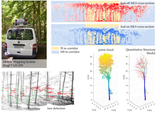
Terrestrial laser scanning (TLS) has been successfully used for three-dimensional (3D) data capture in forests for almost two decades. Beyond the plot-based data capturing capabilities of TLS, vehicle-based mobile laser scanning (MLS) systems have the clear advantage of fast and precise corridor-like 3D data capture, thus providing a much larger coverage within shorter acquisition time. This paper compares and discusses advantages and disadvantages of multi-temporal MLS data acquisition compared to established TLS data recording schemes. In this pilot study on integrated TLS and MLS data processing in a forest, it could be shown that existing TLS data evaluation routines can be used for MLS data processing. Methods of automatic laser scanner data processing for forest inventory parameter determination and quantitative structure model (QSM) generation were tested in two sample plots using data from both scanning methods and from different seasons. TLS in a multi-scan configuration delivers very high-density 3D point clouds, which form a valuable basis for generating high-quality QSMs. The pilot study shows that MLS is able to provide high-quality data for an equivalent determination of relevant forest inventory parameters compared to TLS. Parameters such as tree position, diameter at breast height (DBH) or tree height can be determined from MLS data with an accuracy similar to the accuracy of the parameter derived from TLS data. Results for instance in DBH determination by cylinder fitting yielded a standard deviation of 1.1 cm for trees in TLS data and 3.7 cm in MLS data. However, the resolution of MLS scans was found insufficient for successful QSM generation. The registration of MLS data in forests furthermore requires additional effort in considering effects caused by poor GNSS signal.

1. Introduction

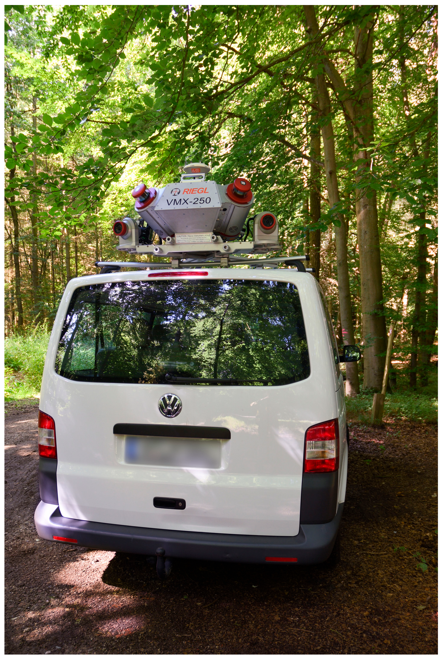
Laser scanning (LS) systems have been used to survey forest structures for almost two decades now [1,2]. Besides airborne laser scanning (ALS) and terrestrial laser scanning (TLS), mobile laser scanning (MLS) is a comparatively new method that has not much been employed and validated in forestry applications so far. MLS is operated from a terrestrial mobile platform (Figure 1) and consists of one or more terrestrial laser scanners in combination with a positioning and orientation system (GNSS and INS) [3]. If motorized vehicles are used as a mobile platform, MLS yields a corridor-like coverage of the surveyed area due to its kinematic capturing along a drivable path or road. However, the drawback of MLS is that the areas reached depend on the forest path with sufficient visibility on the inventory plot in which dendrometrical parameters are to be measured. Also, the range of the laser pulses is strongly influenced by ground vegetation, low branches and foliage. The achievable point densities rank between full area coverage ALS surveys and plot-based TLS surveys. Therefore, MLS combines benefits from both ALS and TLS, but questions remain regarding the quality of this measurement method for forestry applications.

The aim of the work presented here was to investigate the suitability of MLS data for the determination of standard forest inventory parameters as well as for the analysis of crown dimensions. Specifically, this article demonstrates the advantages and disadvantages of multi-temporal MLS data acquisition compared to usual TLS data acquisition. Furthermore, methods of automatic laser scanner data processing tools for dendrometrical parameters (such as diameter at breast height (DBH), tree height, crown projection area (CPA)) are tested in two sample plots using data from different scanning methods (TLS and MLS) and scenarios of foliation (leaf-on, leaf-off). To allow for further ecological analyses, including tree-tree interactions, individual trees are segmented and quantitative structure models (QSM) are extracted and evaluated.

In Section 2 we give a short overview on TLS and MLS for vegetation analyses. Section 3 outlines the study area, the characteristics of the sample plots and the measurement technique used. The methods applied to determine DBH, tree height, CPA and the QSMs are presented in Section 4, followed by the presentation of our results and the discussion.

2. State of the Art

2.1. Terrestrial Laser Scanning in Forestry

Static (or multi-static) TLS recording in forests has become very popular over recent years because it allows dense and accurate three-dimensional (3D) data capturing in forest plots. However, compared to ALS, the area coverage of TLS is small. TLS has been used for plot-based estimation of dendrometrical parameters such as tree position, DBH and tree height [4,5,6]. Furthermore, the high point density allows for a very precise modeling of trunk and branches at the individual tree level [7,8,9,10,11]. Larger areas can be surveyed by combining multiple scans. Van Leeuwen & Nieuwenhuis [12], Dassot et al. [13] and Liang et al. [2] present comprehensive overviews on the application of TLS to extract forest structural parameters. Recently, tree level changes (biomass, spring phenology) have been investigated using multi-temporal TLS datasets [14,15].

2.2. Mobile Laser Scanning for Vegetation Analysis

The main applications of MLS have remained restricted to city mapping or autonomous driving in urban areas, while relatively few studies of mobile mapping for vegetation sampling exist. A basic task in these applications is object recognition in point clouds. Through the detection of vertical cylinder-shaped objects, trees along roads can be detected amongst other objects such as road signs and street lights [16,17,18,19]. Puttonen et al. [20] use MLS data in combination with multi-spectral data of a park and achieve a tree species classification of 10 species with an accuracy of 84%. Liang et al. [21] present the first study on the use of MLS in a large-scale forest area. The extracted tree positions and DBH show accuracies that are close to those of plot-based TLS studies (RMSE of 28 cm and 2.36 cm, respectively). The positioning accuracy of an MLS system is always reduced in forest environments due to the shadowing of the satellites by the canopy and the multipath effects. Qian et al. [22] use the heading angle from GNSS/INS and the velocity data in an IMLE-SLAM algorithm to improve the horizontal accuracy of the trajectory (H-aided IMLE-SLAM with 0.13 m and HV-aided IMLE-SLAM with 0.06 m horizontal accuracy).

In a recent study, backpacks have been used as mobile platforms (personal laser scanning—PLS) [23]. Bauwens et al. [24] compare TLS data (single and multiple scans) with hand-held mobile laser scanner data (HMLS) and present a RMSE of 1.11 cm for the DBHs determined with HMLS. Cabo et al. [25] show similar results for the DBHs comparing a wearable laser scanner (WLS) with TLS data (RMSE of 1.1 cm). However, the RMSE for tree height was much higher and amounted of 9.44 m, which is due to the low range of the WLS. Compared to the vehicle-supported MLS platforms, PLS, WLS and HMLS are cheaper, more flexible and independent of the forest path and the terrain. Unfortunately, the low measurement range and the large beam divergence of the systems studied so far [24,25] are strictly limiting the use in forestry applications. The higher acquisition costs and lower flexibility of MLS systems is balanced by the capturing of corridor-like scan areas within a very short time, which makes it potentially attractive for commercial large-scale data evaluation and forest inventories in large forest stands. A motorized platform also has the advantage that the point cloud is recorded with constant point density.

2.3. Tree Detection and Tree Segmentation from Point Clouds

The successful modeling of individual trees and their crown structures require the detection of each tree in the 3D point cloud data. The fact that this task remains an active field of research illustrates the complexity of this process. When using ALS, the analysis of the digital crown model is the commonly used approach [26]. For TLS data, many algorithms are based on the analysis of horizontal TLS point cloud slices in which the circular-shaped trunks and their respective diameters are detected using the Hough-transformation, or by least-squares fitting circle or ellipse functions [5,27,28,29,30]. The published results of tree detection in single scan data show that the tree detection rate decreases with increasing stem density [2], for example 82% for 153–326 stems/ha [31]; 86.7–100% for 212–410 stems/ha [5]; 73.3% for 358–1042 stems/ha [32], 73.4% for 605–1210 stems/ha [33]. Heinzel & Huber [34] perform a tree detection after a voxel space transformation using morphological operations with shape and neighborhood information (detection rate of 97%).

By placing cylinders into the detected tree positions, an automated tree segmentation can be achieved [5,9]. A disadvantage of this approach is that crowns may not be fully captured (cylinder radius too small) or that adjacent crowns or understory trees are falsely included in the segmentation. A recently published approach of Raumonen et al. [35] employs an automated reliable segmentation of two deciduous tree species based on an algorithm that has been previously developed for tree modeling [10]. For isolated trees common in MLS data of urban areas, methods of segmentation approaches involving stem detection exist. Jaakkola et al. [16] perform a tree segmentation by clustering of vertical line segments and the analysis of their spatial extent. Liang et al. [23] use the eigenvectors of each point and their neighbors to classify trunk points. A horizontal orientation of the normal vector onto the described point cluster is used to classify the points of the trunk. Rutzinger et al. [19] apply a Hough-transformation to remove flat elements (facades) and merge the remaining smaller segments using a connectivity analysis. Zhong et al. [36] present a tree segmentation from MLS data in combination with image data in which overlapping crowns are taken into consideration. After the removal of ground points horizontal slices are analyzed with respect to their spatial extent and point density and finally a tree segmentation is performed. Wu et al. [37] separate adjacent trees based on horizontal voxel layers. Using criteria such as size and perimeter, specific objects (facades, cars, etc.) that do not represent trees are excluded. The differentiation of neighboring crown parts is ultimately performed using a modified region growing algorithm that accounts for distances. Holopainen et al. [38] detect urban trees from TLS, MLS and ALS data using manual, automatic and semi-automatic methods. They report a detection rate of 79% for the manual MLS method. Up to now, there is a lack of suitable methods for fully automatically registering the MLS data obtained in the forest. Moreover, current TLS tree segmentation algorithms require refinement in order to perform well on low resolved MLS point clouds.

2.4. Modeling of Tree Crowns

Eysn et al. [39] divide available algorithms for tree modeling from point clouds into two main types: algorithms using voxel models to represent the woody structure parts of a tree and algorithms that are based on geometric models describing the trunk and branches of a tree as geometric objects, mostly cylinders. A voxel is a regular 3D object, usually a cube with a defined edge length. The inner and shadowed parts of the stem and branches are taken into account when the wood volume is calculated [40,41,42]. Gorte & Pfeifer [7], Pfeifer et al. [43] and Bucksch & Appel van Wageningen [8] use voxel models to segment TLS data prior to skeletonization to identify tree segments. To describe the characteristics of forests, Bienert et al. [44] use voxels to compute probabilities for the reflection of a laser beam based on ray tracing. Geometric models rely on the segmentation of the trunk and branch components. In most cases this segmentation is based on voxel spaces or octree-algorithms. After the segmentation, rotationally symmetric shapes and objects (cylinders, cones, circles) can be fitted into the point cloud segments. Lamprecht et al. [45] use cones, while Pfeifer et al. [43] and Méndez et al. [46] fit cylinders into the primary trunk and branch structures. An automated tree modeling based on cylinders is presented in Raumonen et al. [10,35]. The use of high-resolution TLS and MLS data allows to extract and access multiple crown parameters on the individual tree level, and to measure the angle between branches and their orientation. In Fleck et al. [47] and Bienert et al. [48] the CPA is estimated by calculating the convex hull (closed polygon) of the horizontal projection of the crown points. Lin et al. [49] use MLS to compute crown heights that are applied as ground truth data for the validation of crown height that are derived from panchromatic satellite imagery (WorldView-2). Crown volumes and crown shapes of separated trees can be computed using 3D alpha-shapes [50]. Overlapping crowns and regions of interactions of an individual tree with its neighbors are detected by determining the intersection of alpha-shapes [51,52]. Using a voxel grid approach allows to analyze precisely the spatio-temporal dynamics in canopy space filling at the individual tree and local neighborhood level [53]. Bayer et al. [54] showed that interspecific competition may significantly influence individual tree crown structures. Nevertheless, difficulties remain in the segmentation of crowns in multi-layered stands, where the crowns merge into each other.

3. Datasets

3.1. Study Area

Our study was performed in a natural mixed forest, Lauerholz Forest (53.88° N, 10.74° E), in Northern Germany (Figure 2). The study area covers an area of about 880 ha and is dominated by mixed deciduous forest, with a large number of different tree species (in particular Fagus sylvatica, Quercus robur, Q. petraea, Carpinus betulus, Fraxinus excelsior, Acer pseudoplatanus, A. platanoides, Prunus avium, Ulmus laevis, Alnus glutinosa). In addition, coniferous species are admixed (in particular Pinus sylvestris, Picea abies, Larix decidua, Pseudotsuga menziesii).

3.2. MLS and TLS Data Acquisition

The MLS data was recorded on two dates (March 2017 under leaf-off conditions; August 2017 under leaf-on conditions) using a Riegl VMX-250 Mobile Mapping System (Figure 1). The Mobile Mapping System consists of two Riegl VQ-250 laser scanners as well as an integrated inertial measurement unit (IMU) and global navigation satellite system (GNSS) equipment and six digital cameras. Forest corridors in the study area were captured twice in opposite driving direction (Figure 2). Overall the MLS trajectory had a length of 20.0 km (forest roads in both directions), and data was captured up to 100 m into the forest on each side of the forest road. We recorded the MLS point cloud at a scan rate of 300 kHz (per scanner) at a driving speed of 10–15 km/h. The coverage of the surveyed area thus amounts to about 150 ha. TLS data was recorded at the same time at two plots using a Riegl VZ-400i. We sampled circular 500 m² plots (radius of 12.62 m each). Each plot was scanned from five scanner positions in a multiple scan mode, one in the center of the plots and the other four positions spread in the four cardinal directions with a distance of 15 m from the center, with an angular resolution of 0.05 deg or 0.04 deg, respectively. At the center position, the scanner was tilted by 90° to overcome the limitation of the panoramic field of view. Outside the plot radius, the scanner was tilted by 30°. The instrument height was 1.30 m.

3.3. Sample Plots

The TLS sample plots are located on flat terrain with sparse ground vegetation. The forest path on which the MLS system was used is about 16 m from plot center 1 (Figure 2 and Figure 3). Plot 2 is located in a corner of two forest roads and the plot center has a distance of 16 m and 39 m to the path (Figure 4). The criteria for plot selection were that (i) the plot should lie on a grid point of the manual inventory sampling scheme; (ii) the plot should have less understory at the roadside and should lie close to the path to reduce the extent of occlusion by trees. A total of 24 trees were encountered in plot 1, including Fagus sylvatica with 55% of the plot basal area, Acer pseudoplatanus (25%), Carpinus betulus (15%) and Fraxinus excelsior (5%). A total of 22 trees with a DBH > 7 cm were encountered in plot 2, including Fagus sylvatica with 33% and Quercus petraea with 67% of the plot basal area (based on inventory data of the forestry office of the city of Lübeck from 2013). Plot 2 is characterized by a large number of small understory trees. The stand age of the dominant trees of plot 1 was 103 years and that of plot 2 was 153 years. The DBH was measured crosswise with a caliper from all trees with DBH > 7 cm in plot 1.

Table 1. Characteristics of the different datasets of the sample plots. ¹ The scan resolution depends both on the data rate and on the speed of the mobile platform. ² measured in a 10 cm × 10 cm point cloud slice of a stem facing the trajectory, located 2 m from the plot center.

	TLS		MLS
System	Riegl VZ-400i		Riegl VMX-250
Date	16.03.2017	21.08.2017	14.03.2017	14.08.2017
Foliation	leaf-off	leaf-on	leaf-off	leaf-on
Scan positions (TLS)/records (MLS)	5	5	4	4
Scan resolution 1	0.05 deg	0.04 deg	4.72 m/s	3.33 m/s
Average point density 2	661	700	26	26
Footprint size (plot center)	5.2 mm @ 15 m	5.2 mm @ 15 m	4.9 mm @ 16 m	4.9 mm @ 16 m
Data rate (kHz)	1200	600	300	300
Data points/plot	36.5 M	43.5 M	1.3 M	2.1 M

gives an overview of the laser scanning data of the sample plots.

4. Methods

4.1. Registration of the TLS and MLS Data

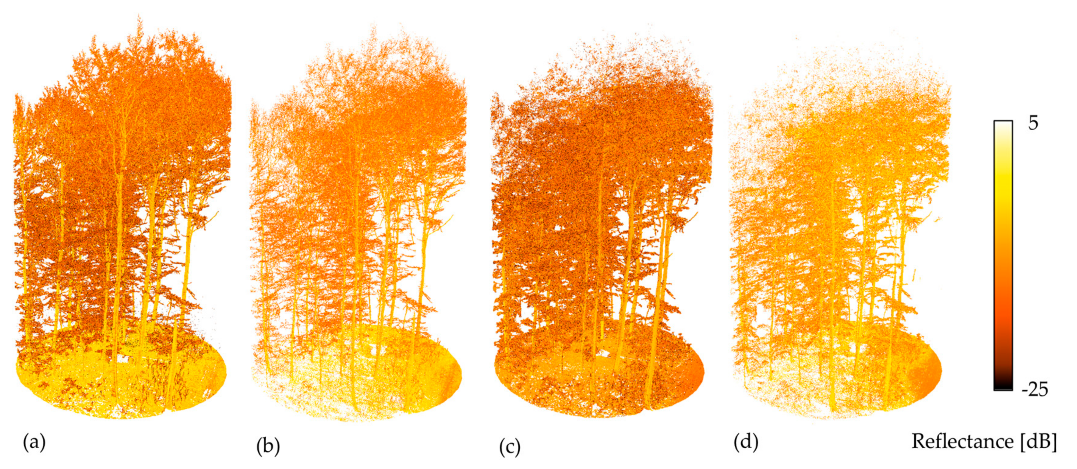
TLS point clouds were co-registered using the registration tools “Automatic Registration 2” and “Multi Station Adjustment” of Riegl RiSCAN Pro 2.6.1. Stray and noise points with a so-called surface reflectance less than −25 dB or a pulse shape deviation greater than 15, both terms defined by the scanner manufacturer [55,56], were removed to achieve a higher quality point cloud. The reflectance value in dB ranges from −25 up to 5, with positive values indicating retro-reflecting targets and negative values are diffusely reflecting targets. For the TLS registration, the point cloud captured in the plot center was used as the project coordinate system and the other four scan positions were registered to the center position. The integrated GNSS sensor in the Riegl VZ-400i enables the global positioning of the scanner positions. Finally, the registered point clouds were exported in the ETRS89/UTM zone 32N coordinate system.

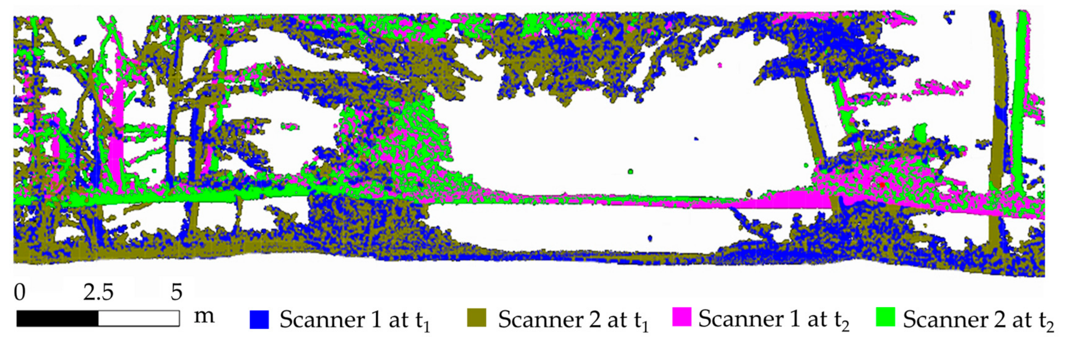
Due to the arising position and height inaccuracy of the trajectory caused by GNSS inaccuracies in forests, the registration of the MLS data requires further data processing. If the forest path is scanned twice from different directions, the trajectory shows differences in position and height (Figure 5). The bigger the time difference between the two scanning events, the larger the influence. The heights and positional deviations registered within the MLS data in the forest were up to 1.8 m in height and up to 1.2 m in position. The RiPRECISION tool from RiPROCESS (1.8.4) was used to eliminate the height error. Since the error is not constantly distributed over the forest path, but instead depends on the quality of the GNSS signals through the canopy, an alternative approach is required. The presentation of the registration algorithm would go beyond the content and topic of this paper and will be presented in a future publication. Finally, the point cloud of Scanner 1 at time t₁ was taken as the reference dataset and the remaining MLS point clouds were transformed to this point cloud.

In order to compare both datasets with each other, a global registration was conducted and the point clouds were transformed to the ETRS89/UTM zone 32N coordinate system and were finally aligned with an ICP algorithm of CloudCompare (version 2.10.alpha).

4.2. Automatic Tree Detection and Forest Inventory Parameter Determination

From the leaf-off TLS and MLS data, an automatic tree detection was performed and forest inventory parameters of interest, such as tree position, DBH and tree height were automatically derived using the method presented in Bienert et al. [57] and Maas et al. [5].

First, the digital terrain model (DTM) is generated with a grid size of s_DTM = 50 cm. Next, tree detection was performed using three horizontal slices with a height h of 1.5, 2 and 2.5 m above the ground. Within the section, a cluster search algorithm and point density analysis are used to search for point accumulations [57]. Point clusters with more than n_min points are stored as potential tree objects. Due to the kinematic recording and the recording direction, the MLS point cloud has a lower point density and the trunks are mapped as circular segments rather than cylinders (see point density in Table 1). To successfully detect point clusters in the less dense MLS point cloud, the minimum number of points (n_min) is increased for the MLS dataset.

For the classification of the point cluster as stem sections, a circle fitting with all cluster points was performed. As exclusion criteria the standard deviation of unit weight (σ₀) and the fitted diameter of the circle fitting are used to classify the tree objects. All detected tree objects are then subjected to a DBH fitting.

In addition, the azimuth and distance of the DBH from the plot center and the 3D coordinates of the circle fitting are stored as tree positions. The tree height is determined by the difference from the highest and lowest Z coordinate of the segmented tree point cloud. This simple difference height determination is only possible when there are no scattering points above the treetops and below the terrain. Since both scan datasets were recorded by a time-of-flight distance measurement, they are free of scatter points.

4.3. Tree Segmentation

The tree segmentation was performed in three steps. First, the trees of the leaf-off TLS point cloud were automatically segmented with the SimpleTree (4.33.06) software, a plugin of Computree (5.0.054b) [58]. Second, the automatically extracted trees were visually inspected, and falsely classified tree segments were manually corrected using RiSCAN PRO software. Third, the extracted trees (i.e., leaf-off TLS) served as the basis for a semi-automatic segmentation of trees from the other datasets (leaf-on TLS, leaf-off and leaf-on MLS).

For the latter we used an approach similar to [44]. The corresponding trees in the other three datasets were segmented using a voxel-template (voxel size of 0.3 m) of the extracted trees. Since all datasets had a uniform reference system, the voxel space of the segmented trees is projected into the point clouds of the other datasets. The points within a voxel form a new tree segment. To account for inaccuracies in transformation and structural changes (leaves, vegetation growth) the points inside the nearest neighbors (1st and 2nd order) of the occupied voxel space are attributed to the segment as a buffer zone. This requires additional manual quality control within the buffer zone. Figure 6 shows the voxel tree template of two example trees within plot 1.

4.4. Quantitative Structure Models

In addition to the classical forest inventory parameters described above, i.e., DBH, tree height, CPA, we quantified the above-ground wood volumes for each extracted tree individual using QSMs. QSMs are a state-of-the-art approach [10,35] to quantify the 3D structure of a tree including its branch topology. In contrast to common allometric equations [59], which mainly use height and DBH, QSMs can deliver a much more accurate estimate of wood volume. QSMs are a description of the tree as a hierarchical collection of geometric primitives (here: cylinders) that are fitted into the point cloud from which topological and geometric tree characteristics can be derived. To generate the QSMs, we used the TREEQSM (2.30) software developed by Raumonen et al. [10] running in Matlab^® (MathWorks, Natick, MA, USA) version R2016a. The method first segments the point cloud of a tree into stem and individual branches and simultaneously determines its topological branching structure. In a second step the method creates a surface and volume model of the segments by fitting cylinders. The segmentation and modeling process is sensitive to specific method parameters [10,11] that, for instance, define the size and number of segments (patches of points) or the minimum/maximum branch diameters that are allowed in the modeling. Therefore, we conducted a parameter optimization test using a subset of three trees (small, medium and large) by comparing the modeled QSMs with the original point cloud. This led to two different sets of parameters. For the TLS point clouds, we used the following parameter values: first minimum patch size: 8 cm; second minimum patch size: 3 cm. For the MLS data we used: first minimum patch size: 9 cm; second minimum patch size: 6 cm. For both datasets we used: second maximum patch size: 6 cm; relative cylinder length: 4; relative radius for outlier removal: 5 [35]. In addition to the QSM we computed the CPA for each tree using a concave hull (alpha-shape with α-value = 0.3) from the projected XY-points [60].

4.5. Data Analysis

To evaluate the results of the parameter determination the root mean square error (RMSE) was calculated and is obtained from Equation (1):

$$RMSE=\sqrt{{\sum }_{i=1}^n\frac{{({\widehat{x}}_i-x_i)}^2}{n}}$$

(1)

with

• n … number of measured values
• ${\widehat{x}}_i$ … measured value
• x_i … measured value from the reference method

The proportion of the values extracted from MLS data to the values of the TLS data is also specified for the determined parameters (x_MLS/x_TLS).

Statistical data analysis of the results was performed with R (3.2) [61].

5. Results

5.1. Registration

Table 2. Accuracies of the MLS and TLS co-registration. ¹ plane-to-plane distance; ² ICP with 3D point-to-point distance; ³ 3D point-to-point distances.

		Plot 1 RMSE (cm)		Plot 2 RMSE (cm)
		Leaf-off	Leaf-on	Leaf-off	Leaf-on
TLS	5 scan positions 1	0.15	0.33	0.27	0.20
	leaf-on to leaf-off 2	1.76		2.58
MLS	forward to backward 3	0.86	0.84	0.54	0.77
	leaf-on to leaf-off 2	2.13		3.57
	TLS leaf-off to MLS leaf-off 2	3.28		3.21

presents the accuracies of the TLS and MLS co-registration. The relative TLS registration was performed with plane patches and standard deviations of a plane-to-plane distance between 0.15 cm and 0.33 cm with RiSCAN Pro 2.6.1. The other datasets show RMSE of 3D point-to-point distances in the range of 0.54 cm up to 3.57 cm.

5.2. Automatic Tree Detection

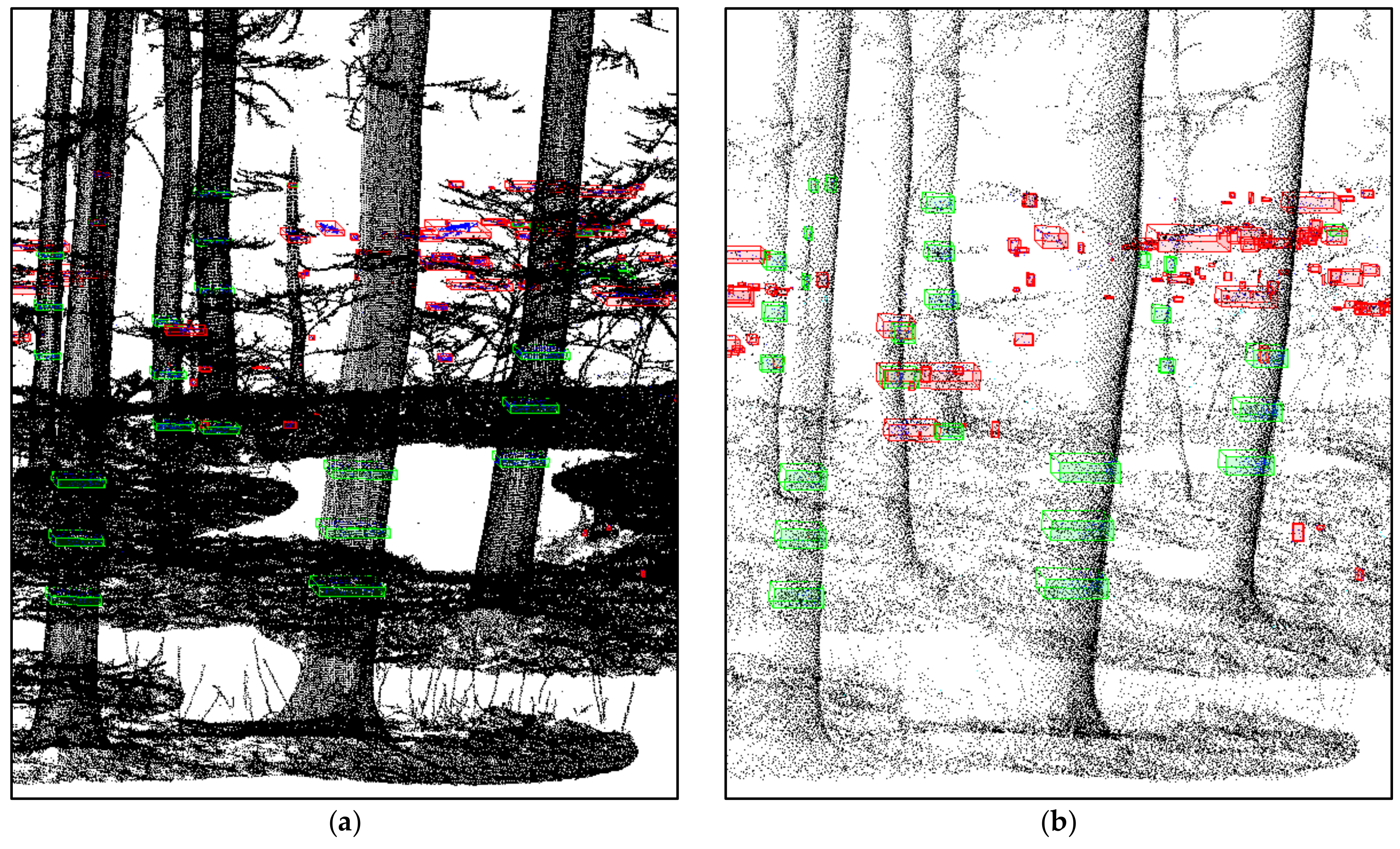
We used a minimum point number for the tree detection (cluster search) in the TLS data of n^TLS_min = 150 and a slice thickness h^TLS_slice of 0.07 m. Finally, all 24 trees were detected in the TLS dataset of plot 1 with three overdetected trees (commission error) (Figure 7). In plot 2, all 22 trees were detected in the TLS dataset. Due to the very high number of young understory trees (Figure 4) 30 commission errors occurred. A zoom-in figure of the point cloud of plot 1 is presented in Appendix A (Figure A1).

The minimum number of points n^MLS_min and the slice thickness h^MLS_slice for tree detection in the MLS data were increased compared to TLS (n^MLS_min = 30, h^MLS_slice = 0.12 m) to avoid a rejection due to the smaller number of points in the horizontal section. Nevertheless, in plot 1 three trees were not detected (12.5% omission error) and eight commission errors occurred. These trees had a DBH < 10 cm and, as a consequence, there were not enough points in the horizontal sections. Figure 7a,b show that the TLS points represent a closed stem section and the MLS points only face the trajectory side of the stem. The missed three trees were detected by manual inspection afterwards, and used to model and compare the tree height, CPAs and QSMs. In plot 2, all trees were detected (no omission error) with 49 overdetected trees. All commission errors in plot 2 originated from the large number of small understory trees.

5.3. Stem Diameter and Tree Height

The DBHs determined with the method of the least squares cylinder fitting are derived from the QSM generation (Section 5.4). The comparison of manually measured DBHs with automatically determined DBHs of the TLS data of plot 1 shows a good agreement with a RMSE of 1.1 cm for the cylinder fitting. The DBHs of the MLS data exhibit an underdetermination (cylinder fit RMSE of 3.7 cm) (Figure 8a). A comparison of the DBHs determined with circle fitting and cylinder fitting is presented in Appendix B.

Table 3. Summary of the proportion DBH_MLS/DBH_TLS of the DBH derived from the QSM of 24 trees (plot 1) and 22 trees (plot 2) determined with TLS and MLS. The two trees from Figure 6 are marked with a green (Carpinus betulus) and red (Fagus sylvatica) color.

Tree	DBH Cylinder Fit Plot 1	DBH Cylinder Fit Plot 2
Carpinus betulus	0.922	-
Fagus sylvatica	0.957	-
Min	0.741	0.741
Max	1.243	1.150
Mean value	0.961	0.906
σ0	0.108	0.115

shows the proportion (DBH_MLS/DBH_TLS) of the DBHs derived from the QSM with cylinder fitting.

The results and the RMSE indicate that the determined tree height based on the MLS data is similar to those from the TLS data and slightly underneath the TLS height estimates (Figure 8b).

5.4. Quantitative Structure Models

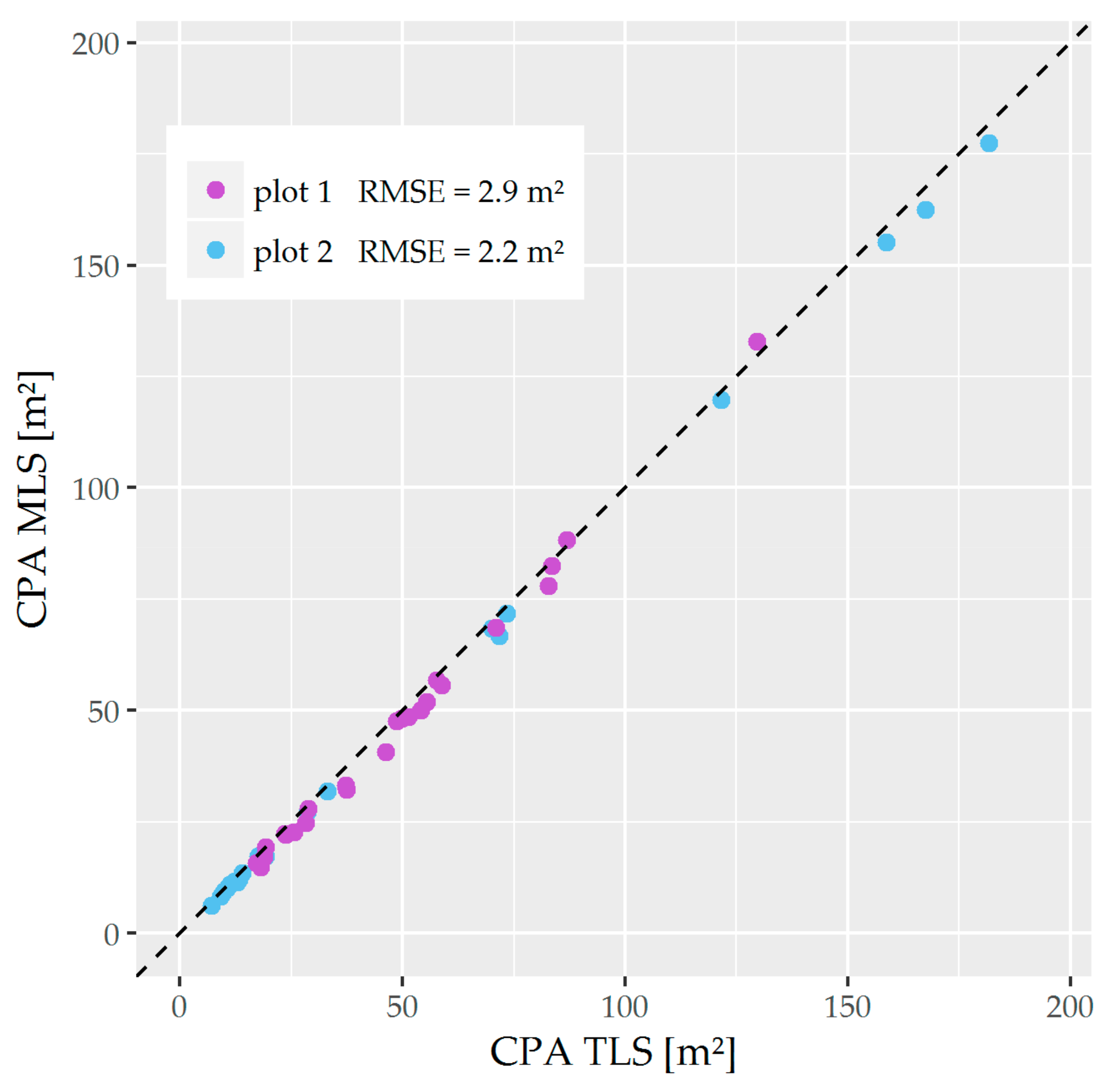
QSMs were generated for all 24 trees of plot 1 and all 22 trees of plot 2 of the TLS and MLS leaf-off datasets. For two trees of plot 1, illustrated in Figure 6, the results are exemplified in more detail. The first one is a Carpinus betulus tree with a height of 18 m and a DBH of 17.5 cm. The tree is positioned 26.3 m from the forest path. The second one is a Fagus sylvatica tree with a height of 32 m and a DBH of 52.7 cm. This tree is placed 7.5 m away from the forest path. Despite the low number of points of the MLS segmented trees compared to the TLS trees (max. 14% of the achieved TLS points), the derived values such as tree height, CPA and DBH show on average only small deviations from the TLS estimated parameters (

Table 4. Summary of the proportion x_MLS/x_TLS of the parameters derived from the QSM of 24 trees of plot 1 and 22 trees of plot 2 determined with TLS and MLS. The two trees from Figure 6 are marked with a green (Carpinus betulus) and red (Fagus sylvatica) color.

Plot 1	Point Number	Tree Height	Total Volume	CPA
Carpinus betulus	0.047	0.953	0.553	0.862
Fagus sylvatica	0.122	0.997	0.72	0.967
Min	0.008	0.894	0.336	0.815
Max	0.143	0.997	1.273	1.025
Mean value	0.055	0.972	0.745	0.938
σ0	0.035	0.022	0.210	0.051
Plot 2	Point Number	Tree Height	Total Volume	CPA
Min	0.033	0.933	0.303	0.875
Max	0.197	0.997	0.850	0.985
Mean value	0.096	0.974	0.463	0.946
σ0	0.043	0.015	0.127	0.033

). A detailed list (

Table A3. Proportion x_MLS/x_TLS of the parameters derived from the QSM of 24 trees of plot 1 determined with TLS and MLS in ascending order with the distance to the trajectory. The two trees from Figure 9 are marked with a green (Carpinus betulus) and red (Fagus sylvatica) color.

Tree Number	Distance to MLS Trajectory (m)	Point Number	DBH Cylinder Fit	Tree Height	CPA	Total Volume	Trunk Volume	Branch Volume
10	6.73	0.095	1.059	0.979	0.938	0.582	0.733	0.424
2	7.46	0.122	0.957	0.997	0.967	0.720	0.841	0.570
13	9.73	0.030	0.945	0.967	0.948	1.095	0.823	1.202
18	9.97	0.046	0.961	0.987	0.926	1.273	0.807	1.778
4	10.29	0.078	0.845	0.972	0.988	0.602	0.861	0.394
17	12.71	0.033	1.243	0.986	1.011	1.199	1.028	1.425
23	12.81	0.143	1.001	0.987	1.025	0.897	0.968	0.810
22	13.01	0.028	0.948	0.935	0.878	0.614	0.788	0.547
6	13.92	0.093	0.926	0.971	0.986	0.688	0.856	0.465
3	14.34	0.046	0.896	0.974	0.943	0.710	0.821	0.672
9	14.52	0.074	0.939	0.987	0.980	0.669	0.901	0.474
21	16.96	0.008	0.952	0.943	0.890	0.602	0.660	0.580
7	17.44	0.109	0.956	0.979	1.015	0.715	0.852	0.483
5	17.55	0.050	1.058	0.972	0.947	0.784	0.866	0.745
19	20.00	0.032	0.824	0.989	0.945	0.650	0.719	0.618
16	20.67	0.038	1.043	0.993	0.917	0.899	0.990	0.658
8	21.59	0.051	1.020	0.973	0.968	0.709	0.862	0.462
12	23.12	0.053	1.192	0.978	0.972	0.336	0.403	0.138
24	23.27	0.012	0.741	0.894	0.889	0.566	0.616	0.550
15	23.35	0.032	0.916	0.963	0.927	0.708	0.855	0.632
14	25.74	0.019	0.948	0.984	0.901	0.873	0.882	0.868
11	25.77	0.044	0.953	0.969	0.815	0.740	0.874	0.342
1	26.31	0.047	0.922	0.953	0.862	0.553	0.853	0.450
20	26.34	0.029	0.808	0.979	0.879	0.616	0.728	0.575

and

Table A4. Proportion x_MLS/x_TLS of the parameters derived from the QSM of 22 trees of plot 2 determined with TLS and MLS in ascending order with the distance to the trajectory.

Tree Number	Distance to MLS Trajectory (m)	Point Number	DBH Cylinder Fit	Tree Height	CPA	Total Volume	Trunk Volume	Branch Volume
18	4.43	0.068	0.845	0.975	0.914	0.320	0.490	0.218
7	4.63	0.183	1.128	0.994	0.985	0.522	0.853	0.244
19	4.71	0.111	0.779	0.986	0.918	0.434	0.608	0.357
20	5.00	0.115	0.743	0.997	0.889	0.372	0.601	0.301
21	5.16	0.096	0.802	0.933	0.951	0.520	0.667	0.425
10	5.30	0.126	0.949	0.978	0.967	0.451	0.638	0.365
22	5.64	0.197	0.836	0.962	0.978	0.350	0.456	0.249
11	5.67	0.141	0.881	0.973	0.966	0.392	0.650	0.300
12	7.17	0.075	0.884	0.983	0.949	0.419	0.675	0.338
17	7.88	0.112	0.868	0.981	0.900	0.433	0.705	0.311
6	8.47	0.036	0.830	0.972	0.954	0.440	0.563	0.344
15	8.54	0.073	0.751	0.961	0.951	0.484	0.638	0.386
9	9.18	0.087	0.925	0.992	0.977	0.689	0.905	0.529
14	9.27	0.091	0.878	0.979	0.985	0.537	0.744	0.456
8	11.44	0.073	1.056	0.987	0.977	0.582	0.905	0.279
13	12.61	0.033	0.911	0.956	0.929	0.510	0.621	0.457
16	12.95	0.037	0.741	0.960	0.875	0.308	0.588	0.218
1	16.02	0.114	1.006	0.982	0.978	0.509	0.900	0.266
4	16.17	0.136	1.150	0.987	0.970	0.849	1.200	0.223
2	16.58	0.085	0.942	0.953	0.977	0.420	0.795	0.197
3	16.66	0.078	1.000	0.975	0.929	0.320	0.661	0.216
5	18.46	0.040	1.036	0.971	0.902	0.303	0.807	0.174

) of the QSM parameters for plot 1 and 2 can be found in Appendix C. The obtained QSMs of the two trees from plot 1 are shown in Figure 9, Figure A3 and Figure A4 in Appendix D. Due to the proportion of the point number, the point clouds in Figure 9c,d look almost the same (0.122), while the point clouds of Figure 9a,b show a clear difference (0.047). The QSMs were generated up to the 5th order branches. The CPA is shown in Figure 10 with a RMSE of 2.9 m² (plot 1) and 2.2 m² (plot 2). It becomes obvious that the MLS extracted CPAs fit well but are slightly underestimated.

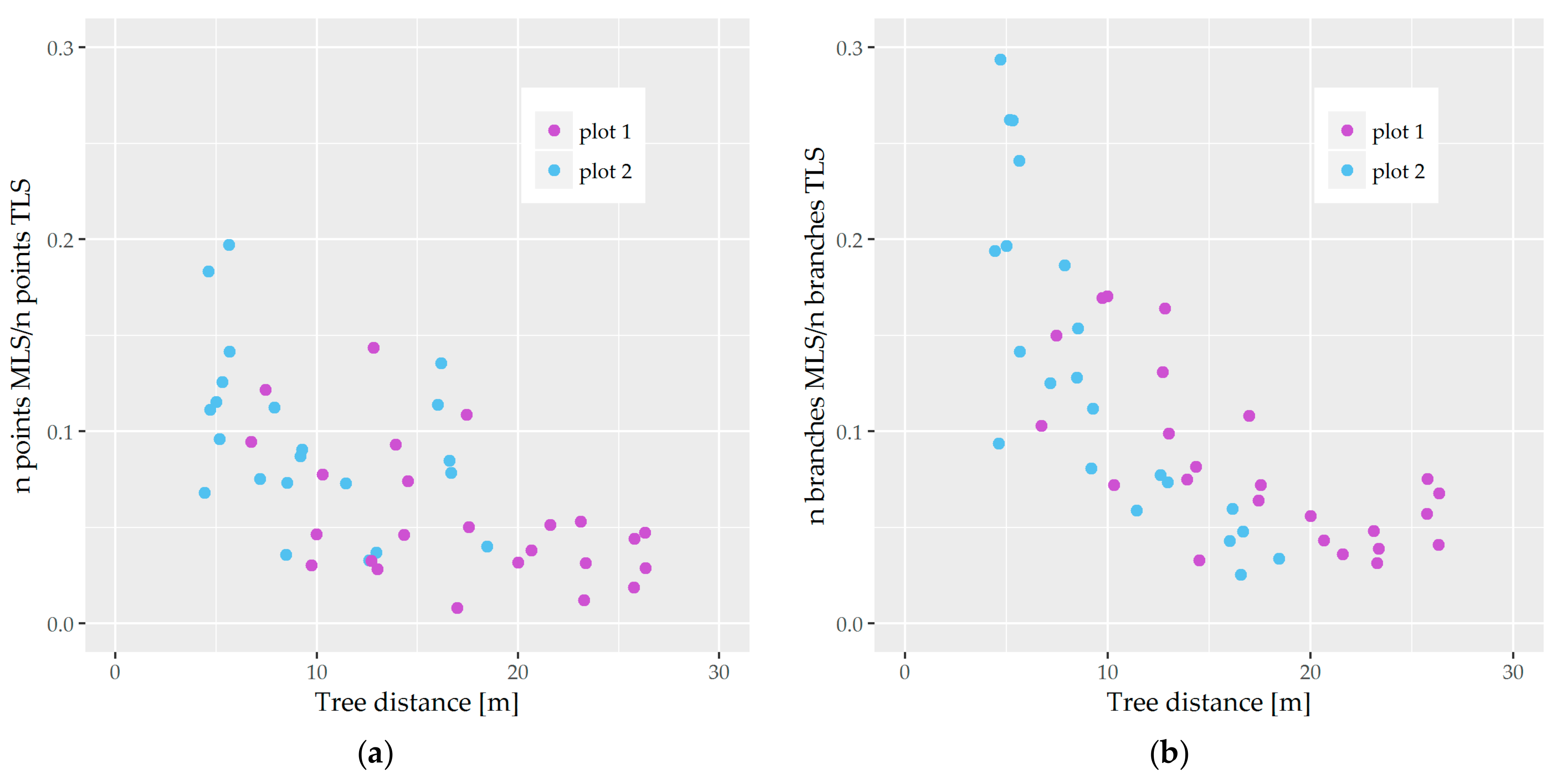
Figure 11a depicts the proportion of the MLS data points to the TLS data points of each segmented tree. The proportion of the number of branches of the MLS to TLS generated by the QSM is shown in Figure 11b. All branches modeled were taken into account. A maximum of 18% (plot 1) and 29% (plot 2) of the branches were modeled from the MLS data compared to the TLS data, which will be reflected in the volume determination. From this analysis it is confirmed that the number of points and the number of extracted branches decreases with increasing distance of a tree from the trajectory. The larger the distance, the larger the point spacing on the scanline and the larger the occlusion effects in the crown area and, as a consequence, the fewer branches can be determined precisely.

The merchantable and total volume of the modeled QSMs are shown in Figure 12a,b. As expected, the volume values show an underestimation of the data derived from MLS. Especially with the larger trees, very large deviations of up to 5 m³ (plot 2) for the total volume were revealed.

5.5. Multi-Temporal Data Acquisition—The Influence of the Vegetation

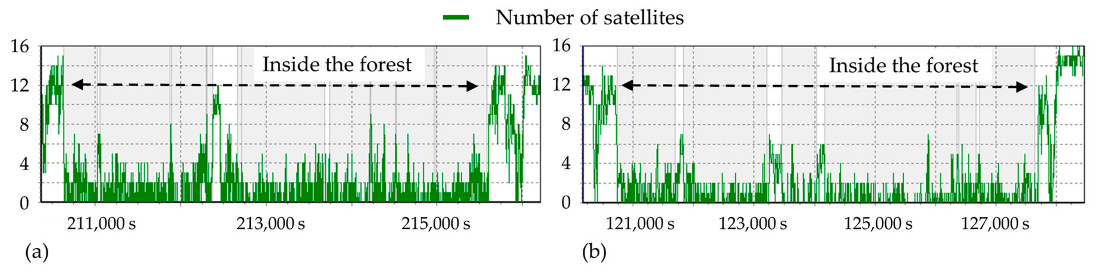
As the study area is in a natural forest with mainly deciduous trees, the aspect of leaf-off and leaf-on conditions has an influence on the point cloud density, on the range of the reflected laser pulses and on the accuracy of the point cloud position. Furthermore, this affects the number of satellites available for GNSS trajectory determination. The comparison of the number of visible satellites shows that under leaf-off conditions more satellites tended to be visible than under leaf-on conditions (Figure 13). The peaks depict larger canopy gaps.

The comparison of multi-temporal TLS and MLS data from a 3 m wide transect under leaf-off and leaf-on conditions shows that the presence of leaves in the summer prevents the laser pulse from reaching the more distant parts of the crown, resulting in less reflections (Figure 14). Furthermore, the weight of the foliage leads to a lowering of the position of the branches in summer.

6. Discussion

The study compared the data quality and information content of TLS and MLS data in a detailed plot analysis. TLS—preferably in a multi-scan configuration to reduce occlusions—delivers very high density point clouds, which form a valuable basis for generating high-quality QSMs. Compared to MLS, the TLS provides a simpler and less expensive way to generate 3D point clouds. On the other hand, MLS offers the possibility of 3D data capture of wide corridor-like areas in even less time due to its mobile platform. We used existing point cloud processing software to derive the parameters from the MLS data. For the registration of multiple-scan forest path MLS data, a suitable software tool capable for nonlinear transformations due to bad or missing GNSS signals is required. Besides the fast and precise 3D recording, MLS also has some challenges compared to TLS. For instance, in this study we used a Mobil Mapping System Riegl VMX-250 mounted on a van, hence the forest paths should have a clear height of 2.8 m to avoid a collision of the MLS-system with branches. Smaller mobile platforms, such as a quad or the use of a PLS/WLS allows to pass through lower vegetation heights. Due to the width of the forest paths, the canopy above the path is often not closed, increasing the light availability for the understory vegetation close to the path. Especially during summer, in a broadleaved or mixed forest a large part of the MLS pulses are blocked by the vegetation next along the path resulting in strong occlusions in the rear trunk and crown space. Driving on skid trails offers an alternative here, since the ground vegetation along the trails will usually be less vigorously developed. However, it is then necessary to use off-road platforms.

In this paper, we have emphasized the acquisition and segmentation of each branch to determine the suitability of MLS for the evaluation of interaction processes between adjacent tree individuals. The tree segmentation procedure used here consists of several interactive steps that are still rather time-consuming. The segmented trees from the SimpleTree tool and the voxel-tree-template must be removed manually via a visual control of adjacent branches. Compared to the voxel-tree-template, the segmented trees from SimpleTree contain only very few neighboring branches, which would theoretically be negligible, but which were cleaned up in the course of evaluation of the interactions processes. Automation can be implemented by means of connectivity analyses in the voxel space, given that the adjacent branches do not fall below a minimum distance and the branches are represented with few occlusions. During the processing chain, an enormous number of occlusions appeared in the crown space of the summer data, so that we have omitted the time-consuming tree segmentation.

The quality of the point cloud registration of the TLS and MLS datasets is less than 1 cm and forms a good basis for the derivation of forest parameters, especially for the stem parameters. The registration of leaf-on to leaf-off datasets shows a lower quality. One reason for this is the foliage. The weight of the leaves pushes the branches down and thus they have been displaced when compared to the leaf-off dataset.

We obtained a RMSE of 3.7 cm for the DBH cylinder fitting in comparison to the manually measured DBHs. The large deviation can be explained by the fact that the trees are 6 to 26 m away from the trajectory and the point density at the trunk is sometimes too low for precise diameter determination. Compared to the high-resolution TLS measurements, the trees have a distance of only 1 to 12 m due to the scanner position in the plot center, which leads to a very high point density. Also Figure 11 shows that with increasing distance of the trees from the trajectory the number of points decreases and thus also the number of modeled branches from the QSM compared to the TLS trees. For MLS campaigns aimed at determining relevant parameters of forest inventories and tree interactions, the distance of plot centers from the trajectory is crucial. The tree species of the stand also has an influence. While pure coniferous stands provide a clear view of the trunks, deciduous or mixed forest stands often show the disadvantage of occlusions in the trunk space due to low branches or tapering. To capture younger trees well, they should be close to the trajectory.

To investigate this aspect more closely, a higher number of plots with at least 250–300 trees is necessary. These should be positioned within the 35 m corridor with different distances from the plot centers to the trajectory. Pure coniferous plots as well as deciduous and mixed forest plots should also be included.

The recording time should be limited to the leaf-off vegetation period if the focus is on the derivation of standard inventory parameters. However, for analysing ecological interactions between individual trees, especially when using QSMs, the resolution of MLS scans will likely be too low. This becomes particularly apparent when comparing QSMs generated from MLS data to those generated from TLS data. Many branches that are important for the interpretation of the interaction between tree individuals are not modeled.

7. Conclusions

In this paper TLS data and MLS survey of a mixed natural forest in different seasons (leaf-off, leaf-on of deciduous trees) were compared with respect to their suitability for applications in forest inventories. The automatic tree detection of the TLS data showed a detection rate of 100% with three commission errors (plot 1) and 100% with 30 commission errors caused by understory trees (plot 2). In comparison, 87.5% of trees were detected in the MLS leaf-off dataset with eight commission errors (plot 1) and 100% of trees with 49 commission errors in plot 2. The DBHs determined with the method of the least squares cylinder fitting are derived from the QSM generation and show a RMSE of 1.1 cm for the TLS data and a RMSE of 3.7 cm for the MLS data. A slightly under-determined MLS tree height in comparison to the TLS tree height (precision: RMSE of 2.0 m of 7 trees measured with a Vertex IV) was detected. Also, the CPAs extracted from the MLS data are slightly under-estimated and show a RMSE of 2.9 m² and 2.2 m² in comparison to the CPAs attained from TLS data. As we compare the MLS to TLS forest parameters the precision of the estimated TLS forest parameters is essential. The precision of the used algorithm to estimate the volume from TLS data shows a slightly mean underestimation of 6% and a R² of 0.90 compared to xylometric reference volumes in one of our previous studies [11]. The merchantable volume obtained from the QSMs show an underestimation of the data derived from MLS (RMSE 0.4 m³ and 0.6 m³). The merchantable volume for smaller trees up to 1 m³ fits very well with the volumes estimated from TLS measurements. Especially with the larger trees, enormous deviations of up to 5 m³ for the total volume (RMSE 1.8 m³) were revealed due to occlusions in the crown space.

The results presented here confirm that parameters derived from MLS point clouds such as tree position, DBH, tree height and CPA are similar to those obtained from TLS, and that the accuracies are within the range of precision required of forest inventory schemes. In future work, several plots along the trajectory will be processed and analyzed at different distances inside the 35 m corridor.

MLS provides rapid and efficient covering of multiple large areas with multi-temporal recordings. The use of MLS in forest science is an emerging field of research. To facilitate a widespread use of MLS in forest research and inventories, future work should concentrate on developing methods for automatic individual tree segmentation and species identification of mixed forests on the basis of existing algorithms, as well as for the precise quantification of canopy space filling and spatio-temporal dynamics in tree-tree interactions for space in the canopy.

References

- Vosselman, G.; Maas, H.-G. Airborne and Terrestrial Laser Scanning; Vosselman, G., Maas, H.-G., Eds.; CRC Press: Boca Raton, FL, USA, 2010; ISBN 978-1-4398-2798-7. [Google Scholar]
- Liang, X.; Kankare, V.; Hyyppä, J.; Wang, Y.; Kukko, A.; Haggrén, H.; Yu, X.; Kaartinen, H.; Jaakkola, A.; Guan, F.; et al. Terrestrial laser scanning in forest inventories. ISPRS J. Photogramm. Remote Sens. 2016, 115, 63–77. [Google Scholar] [CrossRef] [Green Version]
- Graham, L. Mobile Mapping Systems Overview. Photogramm. Eng. Remote Sens. 2010, 76, 222–228. [Google Scholar]
- Thies, M.; Spiecker, H. Evaluation and future prospects of terrestrial laser scanning for standardized forest inventories. Int. Arch. Photogramm. Remote Sens. Spat. Inf. Sci. 2004, 36, 192–197. [Google Scholar]
- Maas, H.-G.; Bienert, A.; Scheller, S.; Keane, E. Automatic forest inventory parameter determination from terrestrial laser scanner data. Int. J. Remote Sens. 2008, 29, 1579–1593. [Google Scholar] [CrossRef]
- Li, Y.; Hess, C.; von Wehrden, H.; Härdtle, W.; von Oheimb, G. Assessing tree dendrometrics in young regenerating plantations using terrestrial laser scanning. Ann. For. Sci. 2014, 71, 453–462. [Google Scholar] [CrossRef]
- Gorte, B.H.; Pfeifer, N. Structuring laser-scanned trees using 3D mathematical morphology. Int. Arch. Photogramm. Remote Sens. Spat. Inf. Sci. 2004, 35, 929–933. [Google Scholar]
- Bucksch, A.; Appel van Wageningen, H. Skeletonization and Segmentation of Point Clouds Using Octrees and Graph Theory. Available online: http://www.isprs.org/proceedings/XXXVI/part5/paper/1252_Dresden06.pdf (accessed on 15 February 2018).
- Schilling, A.; Schmidt, A.; Maas, H.-G. Automatic tree detection and diameter estimation in terrestrial laser scanner point clouds. In Proceedings of the 16th Computer Vision Winter Workshop, Mitterberg, Austria, 2–4 February 2011; pp. 75–83. [Google Scholar]
- Raumonen, P.; Kaasalainen, M.; Åkerblom, M.; Kaasalainen, S.; Kaartinen, H.; Vastaranta, M.; Holopainen, M.; Disney, M.; Lewis, P. Fast automatic precision tree models from terrestrial laser scanner data. Remote Sens. 2013, 5, 491–520. [Google Scholar] [CrossRef]
- Kunz, M.; Hess, C.; Raumonen, P.; Bienert, A.; Hackenberg, J.; Maas, H.G.; Härdtle, W.; Fichtner, A.; von Oheimb, G. Comparison of wood volume estimates of young trees from terrestrial laser scan data. IForest 2017, 10, 451–458. [Google Scholar] [CrossRef] [Green Version]
- Van Leeuwen, M.; Nieuwenhuis, M. Retrieval of forest structural parameters using LiDAR remote sensing. Eur. J. For. Res. 2010, 129, 749–770. [Google Scholar] [CrossRef]
- Dassot, M.; Constant, T.; Fournier, M. The use of terrestrial LiDAR technology in forest science: Application fields, benefits and challenges. Ann. For. Sci. 2011, 68, 959–974. [Google Scholar] [CrossRef]
- Srinivasan, S.; Popescu, S.C.; Eriksson, M.; Sheridan, R.D.; Ku, N.W. Multi-temporal terrestrial laser scanning for modeling tree biomass change. For. Ecol. Manag. 2014, 318, 304–317. [Google Scholar] [CrossRef]
- Calders, K.; Schenkels, T.; Bartholomeus, H.; Armston, J.; Verbesselt, J.; Herold, M. Monitoring spring phenology with high temporal resolution terrestrial LiDAR measurements. Agric. For. Meteorol. 2015, 203, 158–168. [Google Scholar] [CrossRef]
- Jaakkola, A.; Hyyppä, J.; Kukko, A.; Yu, X.; Kaartinen, H.; Lehtomäki, M.; Lin, Y. A low-cost multi-sensoral mobile mapping system and its feasibility for tree measurements. ISPRS J. Photogramm. Remote Sens. 2010, 65, 514–522. [Google Scholar] [CrossRef]
- Lehtomäki, M.; Jaakkola, A.; Hyyppä, J.; Kukko, A.; Kaartinen, H. Detection of vertical pole-like objects in a road environment using vehicle-based laser scanning data. Remote Sens. 2010, 2, 641–664. [Google Scholar] [CrossRef]
- Rutzinger, M.; Pratihast, A.; Oude Elberink, S.J.; Vosselman, G. Detection and modelling of 3D trees from mobile laser scanning data. Int. Arch. Photogramm. Remote Sens. Spat. Inf. Sci. 2010, 38, 520–525. [Google Scholar]
- Rutzinger, M.; Pratihast, A.K.; Oude Elberink, S.J.; Vosselman, G. Tree modelling from mobile laser scanning data-sets. Photogramm. Rec. 2011, 26, 361–372. [Google Scholar] [CrossRef]
- Puttonen, E.; Jaakkola, A.; Litkey, P.; Hyyppä, J. Tree classification with fused mobile laser scanning and hyperspectral data. Sensors 2011, 11, 5158–5182. [Google Scholar] [CrossRef] [PubMed]
- Liang, X.; Hyyppa, J.; Kukko, A.; Kaartinen, H.; Jaakkola, A.; Yu, X. The use of a mobile laser scanning system for mapping large forest plots. IEEE Geosci. Remote Sens. Lett. 2014, 11, 1504–1508. [Google Scholar] [CrossRef]
- Qian, C.; Liu, H.; Tang, J.; Chen, Y.; Kaartinen, H.; Kukko, A.; Zhu, L.; Liang, X.; Chen, L.; Hyyppä, J. An integrated GNSS/INS/LiDAR-SLAM positioning method for highly accurate forest stem mapping. Remote Sens. 2017, 9, 1–16. [Google Scholar] [CrossRef]
- Liang, X.; Kukko, A.; Kaartinen, H.; Hyyppä, J.; Yu, X.; Jaakkola, A.; Wang, Y. Possibilities of a personal laser scanning system for forest mapping and ecosystem services. Sensors 2014, 14, 1228–1248. [Google Scholar] [CrossRef] [PubMed]
- Bauwens, S.; Bartholomeus, H.; Calders, K.; Lejeune, P. Forest inventory with terrestrial LiDAR: A comparison of static and hand-held mobile laser scanning. Forests 2016, 7. [Google Scholar] [CrossRef]
- Cabo, C.; Del Pozo, S.; Rodríguez-Gonzálvez, P.; Ordóñez, C.; González-Aguilera, D. Comparing terrestrial laser scanning (TLS) and wearable laser scanning (WLS) for individual tree modeling at plot level. Remote Sens. 2018, 10, 540. [Google Scholar] [CrossRef]
- Lu, X.; Guo, Q.; Li, W.; Flanagan, J. A bottom-up approach to segment individual deciduous trees using leaf-off lidar point cloud data. ISPRS J. Photogramm. Remote Sens. 2014, 94, 1–12. [Google Scholar] [CrossRef]
- Simonse, M.; Aschoff, T.; Spiecker, H.; Thies, M. Automatic Determination of Forest Inventory Parameters Using Terrestrial Laserscanning. Available online: https://pdfs.semanticscholar.org/9352/c2d6fc676ab612f514f00a857fa9656bc3ec.pdf (accessed on 6 February 2018).
- Aschoff, T.; Thies, M.; Winterhalder, D.; Kretschmer, U.; Spiecker, H. Automatisierte Ableitung von forstlichen Inventurparametern aus terrestrischen Laserscannerdaten. Wissenschaftlich-Technische Jahrestagung DGPF 2004, 15, 341–348. [Google Scholar]
- Henning, J.G.; Radtke, P.J. Ground-based Laser Imaging for Assessing Three-dimensional Forest Canopy Structure. Photogramm. Eng. Remote Sens. 2006, 72, 1349–1358. [Google Scholar] [CrossRef]
- Bienert, A.; Scheller, S.; Keane, E.; Mullooly, G.; Mohan, F. Application of terrestrial laser scanners for the determination of forest inventory parameters. Int. Arch. Photogramm. Remote Sens. Spat. Inf. Sci. 2006, 36, 5. [Google Scholar] [CrossRef]
- Murphy, G.E.; Acuna, M.A.; Dumbrell, I. Tree value and log product yield determination in radiata pine (Pinus radiata) plantations in Australia: Comparisons of terrestrial laser scanning with a forest inventory system and manual measurements. Can. J. For. Res. 2010, 40, 2223–2233. [Google Scholar] [CrossRef]
- Olofsson, K.; Holmgren, J.; Olsson, H. Tree stem and height measurements using terrestrial laser scanning and the RANSAC algorithm. Remote Sens. 2014, 6, 4323–4344. [Google Scholar] [CrossRef]
- Liang, X.; Hyyppä, J. Automatic stem mapping by merging several terrestrial laser scans at the feature and decision levels. Sensors 2013, 13, 1614–1634. [Google Scholar] [CrossRef] [PubMed]
- Heinzel, J.; Huber, M.O. Detecting tree stems from volumetric TLS data in forest environments with rich understory. Remote Sens. 2017, 9. [Google Scholar] [CrossRef]
- Raumonen, P.; Casella, E.; Calders, K.; Murphy, S.; Åkerbloma, M.; Kaasalainen, M. Massive-Scale Tree Modelling From Tls Data. ISPRS Ann. Photogramm. Remote Sens. Spat. Inf. Sci. 2015, II-3/W4, 189–196. [Google Scholar] [CrossRef]
- Zhong, R.; Wei, J.; Su, W.; Chen, Y.F. A method for extracting trees from vehicle-borne laser scanning data. Math. Comput. Model. 2013, 58, 727–736. [Google Scholar] [CrossRef]
- Wu, B.; Yu, B.; Yue, W.; Shu, S.; Tan, W.; Hu, C.; Huang, Y.; Wu, J.; Liu, H. A voxel-based method for automated identification and morphological parameters estimation of individual street trees from mobile laser scanning data. Remote Sens. 2013, 5, 584–611. [Google Scholar] [CrossRef]
- Holopainen, M.; Kankare, V.; Vastaranta, M.; Liang, X.; Lin, Y.; Vaaja, M.; Yu, X.; Hyyppä, J.; Hyyppä, H.; Kaartinen, H.; et al. Tree mapping using airborne, terrestrial and mobile laser scanning - A case study in a heterogeneous urban forest. Urban For. Urban Green. 2013, 12, 546–553. [Google Scholar] [CrossRef]
- Eysn, L.; Pfeifer, N.; Ressl, C.; Hollaus, M.; Grafl, A.; Morsdorf, F. A practical approach for extracting tree models in forest environments based on equirectangular projections of terrestrial laser scans. Remote Sens. 2013, 5, 5424–5448. [Google Scholar] [CrossRef]
- Hosoi, F.; Nakai, Y.; Omasa, K. Voxel tree modeling for estimating leaf area density and woody material volume using 3-D LIDAR data. ISPRS Ann. Photogramm. Remote Sens. Spat. Inf. Sci. 2013, II-5/W2, 115–120. [Google Scholar] [CrossRef]
- Bienert, A.; Hess, C.; Maas, H.-G.; von Oheimb, G. A voxel-based technique to estimate the volume of trees from terrestrial laser scanner data. Int. Arch. Photogramm. Remote Sens. Spat. Inf. Sci. 2014, 40, 101–106. [Google Scholar] [CrossRef]
- Hess, C.; Bienert, A.; Härdtle, W.; Von Oheimb, G. Does tree architectural complexity influence the accuracy of wood volume estimates of single young trees by terrestrial laser scanning? Forests 2015, 6, 3847–3867. [Google Scholar] [CrossRef]
- Pfeifer, N.; Gorte, B.; Winterhalder, D. Automatic reconstruction of single trees from terrestrial laser scanner data. In Proceedings of the XXth ISPRS Congress Technical Commission V, Istanbul, Turkey, 12–23 July 2004; pp. 114–119. [Google Scholar]
- Bienert, A.; Queck, R.; Schmidt, A.; Bernhofer, C.; Maas, H.-G. Voxel space analysis of terrestrial laser scans in forests for wind field monitoring. Int. Arch. Photogramm. Remote Sens. Spat. Inf. Sci. 2010, 38, 92–97. [Google Scholar]
- Lamprecht, S.; Stoffels, J.; Udelhoven, T. VecTree—Konzepte zur 3D Modellierung von Laubbäumen aus terrestrischem Lidar. Photogramm.-Fernerkund.-Geoinf. 2015, 2015, 241–255. [Google Scholar] [CrossRef]
- Méndez, V.; Rosell-Polo, J.R.; Sanz, R.; Escolà, A.; Catalán, H. Deciduous tree reconstruction algorithm based on cylinder fitting from mobile terrestrial laser scanned point clouds. Biosyst. Eng. 2014, 124, 78–88. [Google Scholar] [CrossRef] [Green Version]
- Fleck, S.; Obertreiber, N.; Schmidt, I.; Brauns, M.; Jungkunst, H.F.; Leuschner, C. Terrestrial lidar measurements for analysing canopy structure in an old-growth forest. Int. Arch. Photogramm. Remote Sens. Spat. Inf. Sci. 2007, 36, 125–129. [Google Scholar]
- Bienert, A.; Stiel, B.; Queck, R.; Maas, H.-G. Photogrammetrische Bestimmung von statischen und dynamischen Verformungsstrukturen an Einzelbäumen. Allg. Vermess.-Nachr. 2010, 5, 190–197. [Google Scholar]
- Lin, Y.; Jaakkola, A.; Hyyppä, J.; Kaartinen, H. From TLS to VLS: Biomass estimation at individual tree level. Remote Sens. 2010, 2, 1864–1879. [Google Scholar] [CrossRef]
- Zhu, C.; Zhang, X.; Hu, B.; Jaeger, M. Reconstruction of tree crown shape from scanned data. In Proceedings of the 3rd international conference on Technologies for E-Learning and Digital Entertainment, Nanjing, China, 25–27 June 2008; pp. 745–756. [Google Scholar] [CrossRef]
- Seidel, D.; Leuschner, C.; Müller, A.; Krause, B. Crown plasticity in mixed forests—Quantifying asymmetry as a measure of competition using terrestrial laser scanning. For. Ecol. Manag. 2011, 261, 2123–2132. [Google Scholar] [CrossRef]
- Metz, J.Ô.; Seidel, D.; Schall, P.; Scheffer, D.; Schulze, E.D.; Ammer, C. Crown modeling by terrestrial laser scanning as an approach to assess the effect of aboveground intra- and interspecific competition on tree growth. For. Ecol. Manag. 2013, 310, 275–288. [Google Scholar] [CrossRef]
- Hess, C.; Härdtle, W.; Kunz, M.; Fichtner, A.; von Oheimb, G. A high-resolution approach for the spatio-temporal analysis of forest canopy space using terrestrial laser scanning data. Ecol. Evol. 2018, in press. [Google Scholar] [CrossRef]
- Bayer, D.; Seifert, S.; Pretzsch, H. Structural crown properties of Norway spruce (Picea abies [L.] Karst.) and European beech (Fagus sylvatica [L.]) in mixed versus pure stands revealed by terrestrial laser scanning. Trees 2013, 27, 1035–1047. [Google Scholar] [CrossRef]
- Riegl RIEGL Product Line—Innovations in 3D. Available online: https://user-539731.cld.bz/RIEGL-Online-Catalog-2017-20182 (accessed on 3 March 2018).
- Pfennigbauer, M.; Ullrich, A. Improving quality of laser scanning data acquisition through calibrated amplitude and pulse deviation measurement. In Proceedings of the Laser Radar Technology and Applications XV, Orlando, FL, USA, 5–9 April 2010. [Google Scholar] [CrossRef]
- Bienert, A.; Scheller, S.; Keane, E.; Mohan, F.; Nugent, C. Tree detection and diameter estimations by analysis of forest terrestrial laserscanner point clouds. In Proceedings of the ISPRS Workshop on Laser Scanning, Espoo, Finland, 12–14 September 2007; pp. 50–55. [Google Scholar]
- Hackenberg, J.; Wassenberg, M.; Spiecker, H.; Sun, D. Non destructive method for biomass prediction combining TLS derived tree volume and wood density. Forests 2015, 6, 1274–1300. [Google Scholar] [CrossRef]
- Breu, F.; Guggenbichler, S.; Wollmann, J. Manual for Building Tree Volume and Biomass Allometric Equations: From Field Measurement to Prediction; FAO: Rome, Italy, 2012; ISBN 9789251073476. [Google Scholar]
- Kai, T.; Da, F.; Yvinec, M. 3D Alpha Shapes. Available online: http://www.ics.uci.edu/~dock/manuals/cgal_manual/Alpha_shapes_3/Chapter_main.html (accessed on 6 February 2018).
- Team, R.C. R A Language and Environment for Statistical Computing. 2017. Available online: https://www.r-project.org/ (accessed on 20 January 2018).
Figure 1.
Mobile Mapping System Riegl VMX-250.
Figure 2.
(a,b) Study area with the MLS trajectory (green line) and the two sample plots (red circles). (c) Vertical slice through MLS point cloud under leaf-off or (d) leaf-on conditions with a 35 m (yellow) and 100 m (blue) corridor from the trajectory.
Figure 3.
Point cloud of sample plot 1 with color coded reflectance in dB defined by the scanner manufacturer: (a) TLS leaf-off; (b) MLS leaf-off; (c) TLS leaf-on; (d) MLS leaf-on.
Figure 4.
(a) Leaf-off MLS point cloud of sample plot 2. The dotted line with arrows indicates the MLS trajectory. (b) 3 m wide profile perpendicular to the scan trajectory of the MLS system.
Figure 5.
Cross section of two MLS records (each record has two clouds captured from Scanner 1 and Scanner 2) recorded twice with 30 min time (t1, t2) delay.
Figure 6.
MLS leaf-off point cloud of plot 1 with voxel tree templates extracted with the TLS leaf-off point cloud of a Carpinus betulus tree (green) and a Fagus sylvatica tree (red). Small box: top view. The dotted black line with arrows indicates the MLS trajectory.
Figure 7.
Three horizontal point cloud sections of the tree detection algorithm overlaid with the stem profiles of plot 1 (height interval 15 cm). Point clusters (blue points) detected as ‘tree’ are shown with a green bounding box and rejected point clusters with a red bounding box. (a) leaf-off TLS; (b) leaf-off MLS.
Figure 8.
(a) DBH determination using the MLS and TLS data in comparison with the manually measured diameters; (b) Tree height estimation of the MLS and TLS data.
Figure 9.
Segmented tree point clouds with the extracted QSM of two trees of the leaf-off datasets of plot 1. Top: Carpinus betulus tree (a) TLS; (b) MLS; Bottom: Fagus sylvatica tree (c) TLS; (d) MLS.
Figure 10.
Crown projection area captured from the segmented trees.
Figure 11.
(a) Proportion of MLS point number to TLS point number of the segmented tree point clouds as a function of the distance to the MLS trajectory. (b) Proportion of extracted branch number of the MLS data to the branch number of the TLS data of the segmented trees as a function of the distance to the MLS trajectory.
Figure 12.
Extracted volume of the QSM cylinders: (a) Merchantable volume in (m3); (b) Total volume in (m3).
Figure 13.
Number of satellites during the MLS recording. (a) leaf-off; (b) leaf-on.
Figure 14.
Comparison of the multi-temporal TLS and MLS point clouds of plot 1 on the example of a 3 m wide profile perpendicular to the scan trajectory of the MLS system.