Estimating Individual Tree Height and Diameter at Breast Height (DBH) from Terrestrial Laser Scanning (TLS) Data at Plot Level

Abstract

Abundant and refined structural information under forest canopy can be obtained by using terrestrial laser scanning (TLS) technology. This study explores the methods of using TLS to obtain point cloud data and estimate individual tree height and diameter at breast height (DBH) at plot level in regions with complex terrain. Octree segmentation, connected component labeling and random Hough transform (RHT) are comprehensively used to identify trunks and extract DBH of trees in sample plots, and tree height is extracted based on the growth direction of the trees. The results show that the topography, undergrowth shrubs, and forest density influence the scanning range of the plots and the accuracy of feature extraction. There are differences in the accuracy of the results for different morphological forest species. The extraction accuracy of Yunnan pine forest is the highest (DBH: Root Mean Square Error (RMSE) = 1.17 cm, Tree Height: RMSE = 0.54 m), and that of Quercus semecarpifolia Sm. forest is the lowest (DBH: RMSE = 1.22 cm, Tree Height: RMSE = 1.23 m). At plot scale, with the increase of the mean DBH or tree height in plots, the estimation errors show slight increases, and both DBH and height tend to be underestimated.

1. Introduction

Earth’s forests, which cover 30% of the total land area, are dynamic systems that are constantly in a state of change and drive/respond to the changes taking place in our environment. Tree height, diameter at breast height (DBH) and other forest structure parameters are examples of the important basic data recovered from a traditional forest resource survey. They are of great significance for the research on forest biomass estimation, forest carbon cycle, carbon flow and global climate change. With the development of remote sensing technology, especially the technology of Light Detection and Ranging (LiDAR), many research results have been obtained by using remotely sensed data to extract information on forest structure parameters. There are mainly two ways for estimating parameters of forest structure using traditional passive optical imaging: (1) the correlation between forest structural parameters and spectral information is established by using multi-spectral characteristics of optical remote sensing data [1,2]; and (2) forest structure parameters are extracted using high spatial resolution image texture features [3,4,5]. However, due to the complicated structure of forest canopy cover, atmospheric scattering, and topography, it is difficult for optical remote sensing to provide accurate information about the vertical distribution of the forests [6,7]. As microwaves can penetrate dense canopy to obtain information on the branches and trunks below forest canopies, synthetic aperture radar (SAR) is more advantageous than passive optical remote sensing methods to detect forest structure parameters and biomass [4]. Backscattering mechanism of SAR data [8,9,10] and interferometric synthetic aperture radar (InSAR) [11,12], polarimetric synthetic aperture radar interferometry (POLinSAR) [13,14] and polarization coherence tomography (PCT) [15,16] techniques all have obtained many research results on forest structural parameters. Meanwhile, LiDAR has been intensively applied to the study of forest structural parameters. As space-borne LiDAR can obtain a wide extent of tree height information, it has been applied to studies on large-scale forest biomass [17,18] and forest canopy height [19,20]. However, the new generation of LiDAR satellite ICESat-2 has not yet been launched, and the lack of spaceborne LiDAR data remains a limiting factor [21]. Airborne LiDAR has the ability to obtain the vertical structure of large areas of forest, but it usually cannot reflect detailed structural information under tree canopy [22]. Compared with the above two LiDAR platforms, terrestrial laser scanning (TLS) obtains high density point clouds and can get more detailed information on forest internal structure, including tree location, DBH, tree height, crown width, and other biophysical parameters.

TLS is a laser-based instrument that measures its surroundings using LiDAR for range measurement and precise angular measurements through the optical beam deflection mechanism to derive 3D point observations from the object surfaces [23]. The high-density point cloud data obtained by TLS is widely used and researched in many fields such as engineering surveys [24,25], Earth sciences [26,27], natural disasters [28,29,30], coastline erosion [31,32,33], vegetation monitoring [34,35], and digital terrain mapping [35,36]. In recent years, TLS has been increasingly applied to forest resource surveys, forest management and planning [37,38]. Among a variety of forest structural parameters, DBH and tree height are the most important ones obtained in forest resource surveys. They can provide not only structural parameters of individual trees but also information and data on sample plot level, which are of great significance for the study of forest carbon storage and biomass estimation. Many researchers have conducted investigations on how to extract DBH, tree height and others structural parameters using TLS data efficiently and accurately.

In terms of methodology, the methods for automatically extracting DBH from TLS data mainly include Hough transform [22,39,40], circle fitting algorithm [41,42,43,44,45,46,47], and cylinder fitting algorithm [42,48,49]. Li [40] used the Hough transform method to detect circles on rasterized point cloud data to estimate DBH and tree height. Liu et al. [22] applied the Hough transform method to natural forest and plantation in Puer City, China, and concluded that TLS data could be used to extract DBH (RMSE = 2.18 cm, R² = 0.91). Bienert et al. [41] used a method for fitting circles to extract DBH of trees accurately, and concluded that the tree trunks blocked each other when the tree density was high, which resulted in the reduction of DBH extraction precision or even led to the unrecognizable trees. Moskal et al. [38] used the method of cylindrical fitting to extract DBH, with an RMSE of 9.17 cm. The main reasons for the relatively low accuracy were the poor visibility of the scanning station and the blockage of individual tree trunks. Due to mutual occlusion between the canopy of individual trees, tree heights extracted from TLS point cloud data are always lower than the measured values [22]. The most commonly used method for tree height extraction is to obtain the highest point over the ground within a certain range of a single tree, and use the height of the highest cloud point as the tree height [50]. In order to improve the extraction precision of tree height, most studies have employed the circle fitting method to determine the growth direction of the tree trunk, and calculate the tree height along the growth direction of the tree trunk [22,40,51]. In order to improve the efficiency of the algorithm, the method of extracting DBH based on circle detection or circle fitting needs to rasterize the point cloud data, which reduces the availability of data and the extraction accuracy [22].

As far as study areas are concerned, most of the studies on the extraction of forest structural parameters from TLS data focus on plantations of single forest types or a small amount of natural forests, and research on tree height and DBH extraction of natural forests from typical tree species in a particular area is lacking. Also, most of studies on DBH and tree height inversion have been carried out at scales of individual woods, and studies at scales of forest sample plots with multiple tree species and multi-aged forests are still lacking.

To improve the efficiency and accuracy of forest resource surveys, this study explores methods for extracting tree height and DBH at plot level in complex terrain and different sub-wooded environments using TLS data. Four types of dominant forest species (Pinus yunnanensis Franch., Pinus densata Mast., Picea Mill. & Abies fabri (Mast.) Craib, Quercus semecarpifolia Sm.) are investigated in Shangri-La, northwest of Yunnan, China. Identification of individual trees and extraction of DBH from TLS point cloud data are implemented by using octree segmentation, connected component labeling (CCL) and Random Hough Transform (RHT), following the tree growth direction obtained from TLS point data. Based on the extracted individual tree DBH and tree height, the average DBH and the average tree height are obtained by method of square average.

2. Materials and Methods

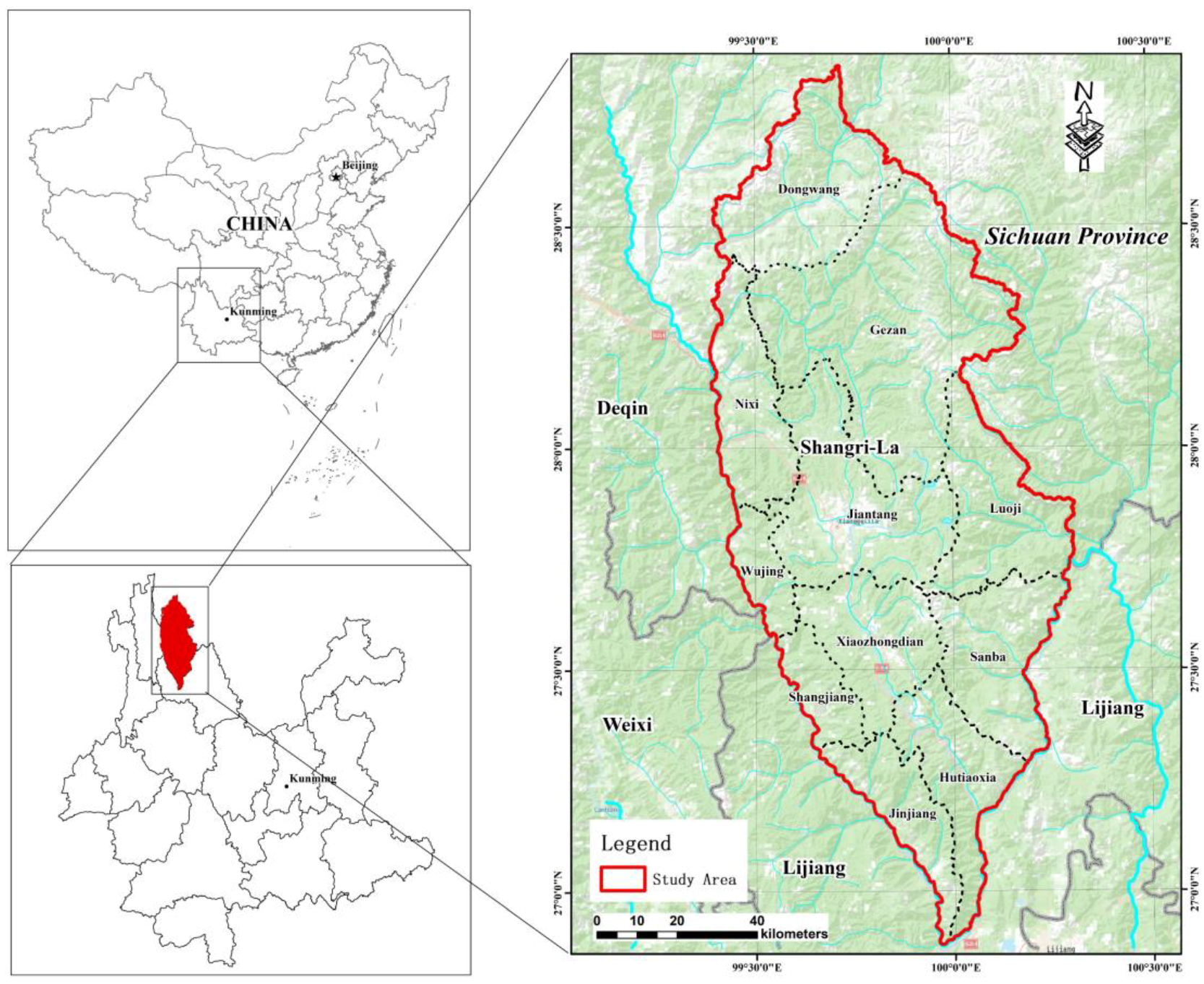
2.1. Study Area and Sample Plots

Shangri-La is located in the northwestern part of Yunnan Province, China, the eastern part of Diqing Tibetan Autonomous Prefecture, between 26°52′~28°52′ N and 99°22′~100°19′ E with an area of 11,613 km². It is one of the largest county-level administrative areas in Yunnan Province (Figure 1). With elevations over 3000 m above sea level in most areas of Shangri-La, the main landform types in the region are subalpine and alpine, which determines the distribution of cold-temperate coniferous forests and temperate-cool coniferous forests in the area. The area of woodland is 962,159.3 hectares in Shangri-La, and total volume of living wood is 133,224,410 m³; the forest coverage rate is 76.00%, and the forest greening rate is 83.19%. Quercus semecarpifolia, Pinus yunnanensis, Pinus densata, and Picea & Abies fabri (including Abies georgei Orr, Abies delavayi Franch., and Picea likiangensis (Franch.) E.Pritz.) account for 90.8% of the total area of arbors in Shangri-La.

This study used the Leica P40 to acquire high-precision 3D point cloud data. The P40 is Leica’s latest generation 3D laser scanning device for fast, high-density point cloud and panoramic image collection. The main performance indicators of the device are shown in

Table 1. Main performance indicators of Leica P40.

Indicators	Descriptions
Range Accuracy	1.2 mm + 10 ppm
3D position Accuracy	3 mm @ 50 m 6 mm @ 100 m
Wavelength	1550nm (invisible); 658 nm (visible)
Scan Rate	Up to 1,000,000 points per second
Field-of-View	360° (Horizontal); 290° (Vertical)
Range and Reflectivity	Minimum range: 0.4 m Maximum range at reflectivity: 120 m (8%), 180 m (18%), 270 m (34%)
Range Noise	0.4 mm RMS at 10 m 0.5 mm RMS at 50 m

.

Point cloud data were obtained at three different times (August 2016, July 2017 and September 2017) respectively. Because the point cloud data of all trees in a sample plot cannot be acquired by only one scanning station, the method of measuring from multiple stations is used in the study. In each plot, five stations (four stations in some samples) were scanned. One station was in the center of the plot with refined scanning method for 10-min scanning, and panoramic photos were obtained at the same time. Other stations were set up on the edge of the sample plot with a 5-min scanning. The study obtained 196 stations of LiDAR point cloud data in 39 forest sample plots (

Table 2. Number of different types of forest sample plots in the study.

Dominant Forest Species	Age of Stand	Number of Sample Plots	Number of Stations	Average Altitude (Unit: m)	Average Slope (Unit: Degree)
Quercus semecarpifolia Sm.	Young	1	5	3892	11.0
	Middle	2	10	3673	15.0
	Mature	1	4	3723	30.0
Pinus densata Mast.	Young	3	17	3225	16.0
	Middle	4	20	3210	16.4
	Mature	2	9	3128	23.5
Pinus yunnanensis Franch.	Young	3	14	2538	19.3
	Middle	5	25	2692	15.3
	Mature	8	43	2316	13.9
Picea Mill. & Abies fabri (Mast.) Craib	Young	2	10	3453	23.3
	Middle	4	20	3604	13.0
	Mature	4	19	3680	15.6

), which were distributed in various townships in Shangri-La (Figure 2).

In order to obtain a sufficient amount of data for verification and ensure the reliability of research results, we used DBH rulers, Trueyard SP1500H laser rangefinder and steel tape to obtain forest structural parameters in all 39 forest sample plots (Figure 2). The range of forest plots varies according to topography and forest density, but the diameter of each plot is not less than 40 m. With the topographical conditions permitting, the range of the sample plot was expanded as much as possible to obtain more data of the tree and to verify the range and accuracy of laser scanning.

2.2. Data Acquisition and Processing

The main research process includes point cloud data preprocessing, normalization of point cloud height, point cloud segmentation, trunk identification, and tree height and DBH extraction. A flowchart detailing the methods in this study is shown in Figure 3. First, a software, Leica Cyclone, is used to stitch multi-site point cloud data based on the Leica 4.5″ circular black & white target. Because there is a lot of redundancy in multi-site point cloud data, the software also is used to deduct data so that we can reduce the time cost in data processing under the premise of ensuring data extraction accuracy.

2.2.1. Normalization of Point Cloud Height

A morphological filtering method [52] is used to separate ground points from non-ground points. The main idea of morphological filtering is to use the corrosion and expansion operations in mathematical morphology to remove the higher point cloud in the point cloud and keep the lower point cloud to achieve the purpose of extracting ground points [53]. Ground points are interpolated and meshed by Inverse Distance Weighting (IDW) method. Finally, using the generated grid of ground, points heights are normalized to eliminate the difference in tree height caused by differences in elevation (Figure 4).

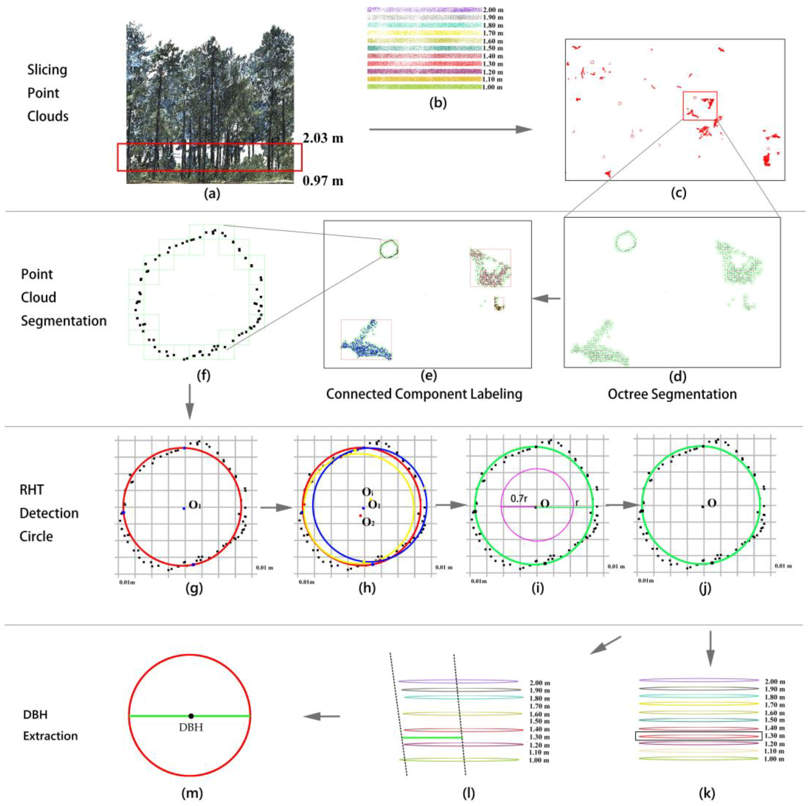
2.2.2. Slicing Point Clouds

When obtaining 3D point cloud data in forest sample plots with higher density trees or undergrowth shrubs, it is more likely that trees will block one another and undergrowth shrubs will block the trunks, producing incomplete point cloud data at a certain height which leads to missing or misidentification of trees. Several studies [22,40,42] have shown that the method of slicing point clouds can effectively improve accuracy of octree identification. Unlike existing studies using hierarchical rasterization of collected point clouds, this research directly deals with point cloud data to ensure the accuracy of point clouds and make full use of all acquired data. The thickness of each layer of point cloud is also an important factor that affects tree identification and DBH estimation. In order to ensure the accuracy of DBH estimation, tree diameters were calculated at 1.3 m using multi-layer thickness of point clouds, and the accuracy results are shown in

Table 3. Point Cloud Thickness and Accuracy.

Thickness (cm)	RMSE 1	Number of Trees Detected Correctly	Number of Trees Undetected	Error Detection 2
1.00	2.92	53	27	22
2.00	3.04	63	17	20
3.00	2.58	75	5	29
4.00	2.99	74	6	14
5.00	2.57	74	6	8
6.00	2.33	75	5	5
7.00	2.53	75	5	7
8.00	2.62	78	2	17
9.00	2.65	78	2	15
10.00	2.74	76	4	12

¹ RMSE: Root mean square error compared with the measurement result; ² Error Detection: Number of misidentified trees compared with manual recognition.

.

It can be seen from Table 3 that, when the thickness of slicing point cloud is 6 cm, the RMSE of individual tree DBH is the smallest (2.33 cm). Therefore, point clouds at 0.97 m–2.03 m are sliced into 11 layers with an interval of 0.10 m and a thickness of 0.06 m (0.97 m–1.03 m, 1.07 m–1.13 m, 1.17 m–1.23 m, 1.27 m–1.33 m, 1.37 m–1.43 m, 1.47 m–1.53 m, 1.57 m–1.63 m, 1.67 m–1.73 m, 1.77 m–1.83 m, 1.87 m–1.93 m and 1.97 m–2.03 m).

2.2.3. Octree Segmentation and Connected Component Labeling

In order to reduce redundancy and improve processing efficiency and accuracy, octree segmentation and connected component labeling are combined to segment the point clouds before trunks are identified.

The method of connected component labeling [54] is usually used to detect connected areas of binary images in the field of computer vision. It can be used for processing color images and higher dimensional data as well. Different from the image data, point cloud data is composed of a large number of independent, discrete points with spatial coordinates. Therefore, the method of octree segmentation is used to obtain voxelization data of the hierarchical point cloud. Voxelization is a processing of point cloud segmentation based on octree. First, a closed minimal cube is determined as a root node or a zero-level node, and then the root node is subdivided into eight voxels recursively. Non-empty voxels continue to be divided until they are divided into the remaining thresholds or the minimum pixel size criteria are reached [55].

As shown in Figure 5, the raw point cloud contains a large number of useless points (shrubs, weeds, etc.). With the increasing depth of octree (Figure 5b–h), the points are divided into relatively independent spaces. When the octree level = 10, trunks, shrubs and weeds show better separability. By further increasing the depth of the octree (Octree level = 11 or Octree level = 12), the original separability between the trees is maintained, but the amount of data has increased substantially. Therefore, this study uses the octree segmentation method with octree level = 10 to voxelize each layer of cloud data of trunks. Based on voxelization of points, we use the method of connected component labeling to get point cloud voxels connected and complete the segmentation of tree stem form stratified point clouds. The segmentation results are shown in Figure 5i.

2.2.4. Random Hough Transform and DBH Extraction

The detailed process of extracting DBH using random Hough transform is shown in Figure 6. For sliced point cloud data, the RHT method is used to sequentially perform circular detection from multiple sub-regions in each layer respectively until extraction of all sliced point cloud is completed. The process of extracting each sub-partition (point cloud set P) of each layer is as follows:

(1)

First, the point set P is projected onto the X–Y plane in the direction of Z-axis to form a 2-D point cloud set P′ (Figure 6f). Defining the Hough space M (m, n, r) is carried out, where m is the number of grids with 0.01 m intervals for point cloud set P’ in the direction of X-axis, n is the number of grids with 0.01 m intervals for P′ in the direction of Y-axis, and r is the radius stored in millimeters (Figure 6g, the gray grid under points). Three points p₁(x₁, y₁), p₂(x₂, y₂), p₃(x₃, y₃) that are non-collinear and where the distance between any two points is greater than 0.02 m are selected from the point cloud set P’ randomly. The condition of three non-collinear points p₁(x₁, y₁), p₂(x₂, y₂), p₃(x₃, y₃) can be expressed as:

$$\left|\begin{array}{ccc}x-x_1& y-y_1& z-z_1\\ x_2-x_1& y_2-y_1& z_2-z_1\\ x_3-x_1& y_3-y_1& z_3-z_1\end{array}\right|=0$$

(1)

The distance conditions between the points are:

$$\begin{gathered} \sqrt{{\left(x_1-x_2\right)}^2+{\left(y_1-y_2\right)}^2}>0.02 \\ \sqrt{{\left(x_1-x_3\right)}^2+{\left(y_1-y_3\right)}^2}>0.02 \\ \sqrt{{\left(x_2-x_3\right)}^2+{\left(y_2-y_3\right)}^2}>0.02 \end{gathered}$$

(2)

Then, these 3 points can form a circle C₁, with the center point O₁ (a₁, b₁) (Figure 6g) and the radius r₁ of the circle can be obtained. According to our field survey results, if r₁ > 0.7 or r₁ < 0.03 (trees with DBH larger than 1.40 m or less than 0.06 m are not extracted), a new set of three points should be selected for calculating the radius r_i until r_i satisfies 0.03 $\le$ r_i $\le$0.7. The corresponding Hough parameter space is voted in as M(a_i,b_i,r_i) = M(a_i,b_i,r_i) + 1.

(2)

This method is repeatedly performed on the remaining point clouds until the elements in P′ are depleted, so that the final M is obtained. If the difference between the radii of two concentric circles in M is less than 0.01 m, the circles are considered to be the same circle, the average radius of all concentric circles is used as the final radius, and the final voting result is the sum of all circles that meet the conditions. Formula (3) expresses the voting result in M:

$$\frac{M\left(a_i,b_i,r_i\right)}{\max \left(M\right)}>\mathsf{\epsilon }$$

(3)

where, ε is the threshold value of a circle detected for sliced point cloud of trees. Many tests in the study show that the accuracy of DBH extraction is high when ε = 0.80. The next condition needing to be tested is the relative position between any point (x_i,y_i) in point cloud P’ and the circle C_i (a_i,b_i,r_i) satisfying the voting result in M:

$$\sqrt{{\left(x_i-a_i\right)}^2+{\left(y_i-b_i\right)}^2}<0.7\times r_i$$

(4)

Equation (4) indicates that there are points inside the identified trunk, which are inconsistent with the actual results and should be excluded from the circle that satisfies the voting result.

(3)

Using this method, all layers of point clouds are extracted, and the trunk position and the trunk section radius of each layer of trees are obtained. If the position of tree trunk is detected in four or more layers, it is assumed that there is a tree at this position, and the single-wood position is the center of the trunk closest to the ground. If a trunk can be accurately identified at a height of 1.30 m, DBH of the tree is diameter of the circle identified (Figure 6k). If the trunk cannot be identified, the linear regression method is used to fit the trunk radius and trunk height to obtain DBH (Figure 6i).

2.2.5. Tree Height Extraction

According to the field surveys, trees in most sample plots in the study area grow in a vertical direction and the trunks are relatively straight. Using the extracted tree locations, point clouds are sliced at an interval of 1.00 m with a thickness of 0.06 m. The RHT method is used to obtain the diameter of multi-layer trunks and the centers of the circles, and the multi-layer centers of circles are used to fit a straight line in the space, which is the growth direction of the tree. Based on the different DBH of each tree, the point clouds are cropped from the bottom to the top along the fitted line within a certain range. These point clouds are considered to be from the same tree, and the height of the tree is considered to be the height of the highest point of all points. However, for sample plots with higher density of forest trees, this method cannot be applied to the lower trees because there may be point clouds of other trees along the growth direction of the trunk, as shown in Figure 7a. To handle such situations, Liu et al. [22] adopted a method of vertical detection along the growth direction of the trunk to calculate the tree height of the lower tree by counting the changes in the voxel of the point cloud. However, the method can only reflect the change of the number of point clouds in the direction of Z-axis, and cannot accurately stratify the different levels of trees. In order to detect the attributions of the tree point cloud effectively, extracted tree points (Figure 7b) are segmented using the CCL method based on the octree segmentation described previously. The segmentation result is shown in Figure 7c. It can be seen from Figure 7c that the algorithm separates points of the low tree and points of high-level tree accurately, and the height of the low tree can be obtained from the highest z value of the segmented tree.

3. Results and Discussion

3.1. Analysis of the Influence of Forest Density on Scanning Range and Accuracy

Forest point clouds collected by TLS are often affected by mutual shelter between trees. Mutual obstruction between trunks results in lower accuracy in tree segmentation and DBH extraction, while mutual shelter between canopies leads to lower accuracy of tree height extraction. From Table 1, it can be seen that the Leica P40 can obtain a large range of high-precision 3D data. However, due to the shelter between trees, the extent of scanning is limited, and the density of trees in forest limits the size of forest sample plots. In order to ensure the accuracy of tree height and DBH extraction, three typical sample plots of Pinus yunnanensis (plot numbers 20170726012, 20160831017 and 20160824002) are selected to analyze the accuracy of the same tree species with different forest density (

Table 4. Effects of Forest Density and Distance on Scanning Range and Accuracy.

Plot #	Stand Age	Mean DBH	Mean T.H.1	<5 m				5 m–10 m
				RMSE		Trees Num.	ER Trees2	RMSE		Trees Num.	ER Trees
				DBH	T.H.			DBH	T.H.
20170726012	Young	11.30	8.2	0.91	0.41	13	0	1.09	0.44	43	7
20160831017	Middle-age	24.70	15.2	1.27	0.54	2	0	1.20	0.89	18	0
20160824002	Mature	28.40	18.0	0.68	0.59	2	0	1.64	0.46	6	0
10 m–15 m				15–20 m				>20 m
RMSE		Trees Num	ER Trees	RMSE		Trees Num.	ER Trees	RMSE		Trees Num.	ER Trees
DBH	T.H.			DBH	T.H.			DBH	T.H.
0.81	0.57	43	0	1.30	0.60	12	35	–	–	□	–
1.28	0.56	18	1	1.36	0.30	26	1	1.33	0.78	218	30
1.64	0.52	10	2	1.00	0.17	18	2	1.43	0.84	40	11

¹ T.H.: Tree Height; ² ER Trees: Error trees, misidentified trees.

). According to the result of that, we can determine a range of sample plots suitable.

It can be seen from Figure 8 and Table 4 that topography and forest density affect the scanning range and scanning accuracy of the terrestrial laser scanner.

(1)

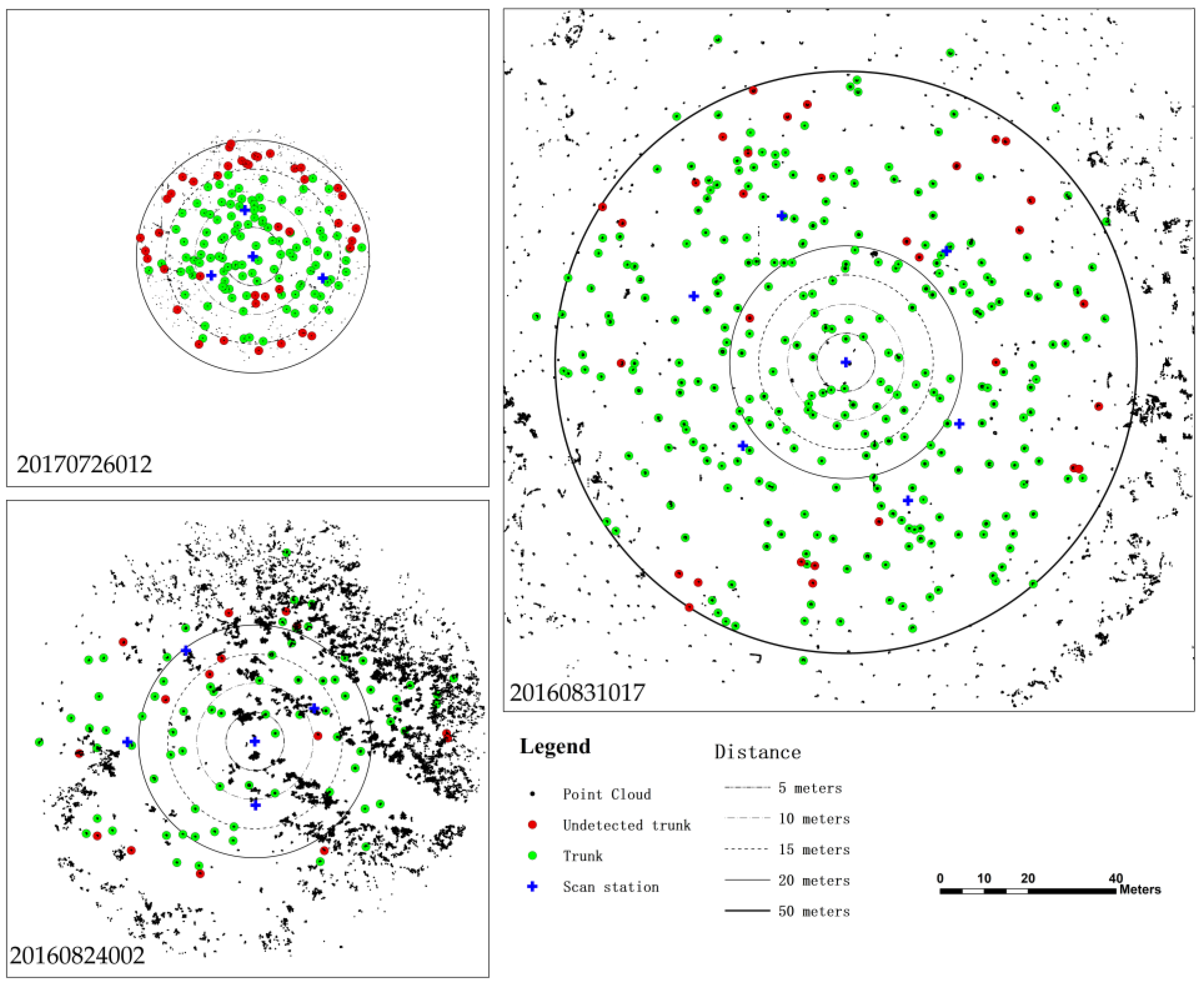
The scanning range of high-density young forest sample plots is seriously affected by the mutual obstruction between trees. Trees can be identified more accurately (99/106) within a range of 15 m centered on the central station, but there are a small number of missing trees (7 trees) due to mutual shelter between trees within the forest sample plot (5 m–10 m). The identification accuracy of trees near the edge of the young sample plot (distance from the center of the sample plot > 15 m) is low, and there are a large number of missed trees (35). The DBH and extraction accuracy of tree height of the entire sample plot is relatively high (mean RMSE of DBH is 1.03 cm, and mean RMSE of the tree height is 0.51 m). The maximum error is also located near the edge of the sample plot.

(2)

The scanning range of the medium–density plot is mainly affected by the topography and low bushes under the forest canopy. In areas with low tree density and relatively flat terrain, a larger range of scanning areas can be obtained and the accuracy of tree identification and height/DBH extraction are higher as well. For the sample plot of NO. 20160831017, within the range of 20 m from the center of the sample plot, 64 out of 66 trees are identified, with an RMSE of 1.28 cm for DBH, and an RMSE of 0.57 m for tree height. When the distance from the tree to the center of the sample plot exceeds 20 m, the tree recognition accuracy decreases slightly. The tree height and DBH extraction accuracy also slightly decreases with the increase of the distance from the tree to the center of the sample plot.

(3)

Low–density mature forests have a relatively complete vertical structure of individual trees. The growth space under the forest canopy is sufficient for the growth of low shrubs. It can be seen from the point clouds (Plot 20160824002) that a large number of shrub points are included in the point cloud near the ground. Meanwhile, the effective range of sample plots obtained by multi–station scanning is limited due to terrain influences. It can be seen from Table 4 that extraction results obtained within the range of 20 m is better than those beyond the range: The tree detection rate is high (36/40), with an RMSE of 1.24 cm for DBH, and an RMSE of 0.46 m for tree height. When the distance from the tree to the TLS scanner is more than 20 m, the accuracy of tree detection is slightly reduced (40/51) due to the longer distance and the influence of shrubs around the station.

3.2. Analysis of the Influence of Forest Types on the Accuracy of Results

The morphological characteristics of forest trees often change with forest species, forest age and growing environment. Pinus yunnanensis and Pinus densata are genus Pinus, and their trunks are mostly straight–lined and their crowns clustered (Figure 9a,b). The trunk of Picea and Abies fabri grows upright and the lateral branches grow into the surrounding layers. The shape of the tree crown shows an approximate cone (Figure 9c). Quercus semecarpifolia is significantly different in morphology from the other three tree species, with a more curved trunk and wider coverage of the crown (Figure 9d). The young, middle-aged and mature forest sample plots of the four types of dominant forest species are selected to analyze the differences in extraction accuracy of tree height and DBH for different forest types and different tree shapes.

(1) The influence of forest types on DBH extraction accuracy

It can be seen from Figure 10 that the accuracy of DBH extracted from point cloud data of four main tree species is very high using the method described in Figure 3, with an average RMSE of 1.28 cm, and a minimum error of 1.17 cm for Pinus yunnanensis. The RMSE of DBH extracted is 1.52 cm, but the correlation is highest among all forest types (R² = 0.986). It can be seen from Figure 9 that the four tree species have different morphologies, but the trunks are all nearly circular and are mostly straight near the ground. The results suggest that it is conducive to use the RHT method to extract DBH.

(2) The effect of tree species on tree height extraction accuracy

Several studies [38,56,57] have shown that the extraction of forest trees by TLS cannot obtain the point cloud information at the top of the canopy due to the mutual occlusion between canopies, which leads to an underestimation of tree height. The forest in the study area is mainly coniferous with some broad-leaved trees. Compared with broadleaf forests, coniferous forest canopy has some voids, and relatively accurate tree heights can be obtained in a certain range when the stations are properly arranged. It can be seen from Figure 10 that the largest underestimation of tree height is from Picea & Abies fabri (RMSE = 1.28 m), followed by Quercus semecarpifolia, Pinus densata and Pinus yunanensis. The mean RMSE of 4 species is 0.95 m, and all of them showed good correlation.

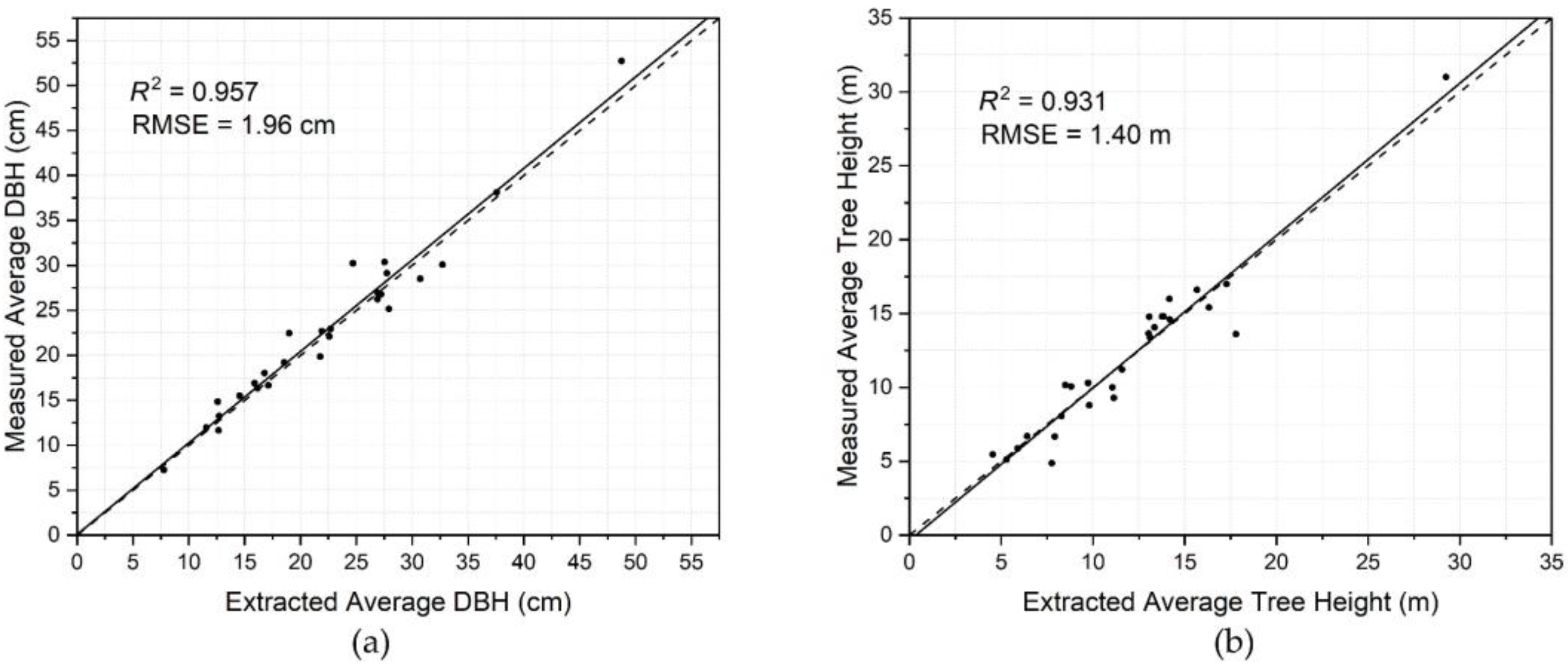
3.3. Accuracy Analysis of Results in Forest Sample Plots

Major elements of forest surveys include tree diameter, height, coverage, and density, among which the tree height and diameter are the most important ones. Mean DBH is the diameter corresponding to the average basal area of dominant tree species, which is a basic index reflecting the forest roughness. The methods of calculating mean DBH include the arithmetic mean method, quadratic mean method, volume mean method, mode method, and median method. At present, the method of quadratic mean is commonly used in forest surveys:

$$\overline{D}=\sqrt{\frac{\sum d_i^2}{n}}$$

(5)

where, $\overline{\mathrm{D}}$ is the mean DBH, d_i is the DBH of tree i, and n is the total number of trees in forest sample plots.

The mean stand height is an important indicator that reflects the height level of stands, and it is an important tree parameter in forest surveys. For the measurement of arborous forest, it should be determined by selecting 3 to 5 average sample trees among the main forest layer dominant tree species according to the average DBH, and the average tree height should be calculated using the arithmetic mean method.

In this paper, the mean DBH and mean stand height are calculated by using the methods above, and compared with the measured data in sample plots for accuracy assessment. It can be seen from Figure 11 that the mean DBH and mean tree height extracted by the RHT method combined with octree segmentation have strong correlations (correlation of DBH is R² = 0.957, correlation of tree height is R² = 0.905) with the measured data. The mean RMSE of the extracting method is 1.96 cm. The smaller the mean DBH, the higher the extraction accuracy. With the increase of the mean DBH in plots, the errors tend to increase slightly. The RMSE of the extracted mean stand height is 1.40 m. Because the canopy obscures the point cloud, results of tree height extracted by TLS data are slightly lower than the actual tree height in forest sample plots with higher average tree heights.

4. Conclusions

The study focused on extracting tree height and DBH data of natural forest species at plot level in Shangri-La, Northwest Yunnan, China. Combining methods of octree segmentation, CCL and RHT algorithm, tree heights and DBH of natural forests at individual tree level and plot level were obtained. Topography, understory shrubs and tree density influence the TLS scanning range and accuracy of results. Because of different morphology of different tree species in Shangri-La, the accuracy of tree height and DBH extraction for different tree species is different using the method. In general, Pinus yunnanensis, Pinus densata and Picea & Abies fabria are coniferous forests, with vertical trunks and similar morphological structures and tree height extraction precision is high. Quercus semecarpifolia is a broad–leaved forest species, and its morphology is different from that of coniferous forest, leading to relatively low extraction accuracy. In general, the methods used in the study have high accuracy for the extraction of DBH and tree height for four dominant tree species in Shangri-La. The average RMSE of DBH is 1.28 cm, and the average RMSE of tree height is 0.95 m. The results at forest sample plot levels also show that the method can obtain the mean tree height and mean DBH accurately in complex terrains. In the last few years, mobile/personal laser scanning and image-based techniques have become capable of providing similar 3D point cloud data, and have their own advantages, e.g., lower cost when using image-based techniques and high efficiency when using mobile/personal laser scanning. Further studies need to demonstrate the added value of using TLS, which most probably comes from the highly accurate tree attribute estimates.

References

1. Wu, D.; Li, B.; Yang, A. Estimation of tree height and biomass based on long time series data of landsat. Eng. Surv. Mapp. 2017, 1–5. [Google Scholar] [CrossRef]
2. Lu, D. Aboveground biomass estimation using landsat TM data in the Brazilian amazon. Int. J. Remote Sens. 2005, 26, 2509–2525. [Google Scholar] [CrossRef]
3. Liu, X.; Dan, Z.; Xing, Y. Study on Crown Diameter Extraction and Tree Height Inversion Based on High-resolution Images of UAV. Cent. South For. Invent. Plan. 2017, 36, 39–43. [Google Scholar] [CrossRef]
4. Dong, L. New Development of Forest Canopy Height Remote Sensing. Remote Sens. Technol. Appl. 2016, 31, 833–845. [Google Scholar] [CrossRef]
5. Ozdemir, I.; Karnieli, A. Predicting forest structural parameters using the image texture derived from worldview-2 multispectral imagery in a dryland forest, Israel. Int. J. Appl. Earth Obs. Geoinform. 2011, 13, 701–710. [Google Scholar] [CrossRef]
6. Gibbs, H.K.; Brown, S.; Niles, J.O.; Foley, J.A. Monitoring and estimating tropical forest carbon stocks: Making redd a reality. Environ. Res. Lett. 2007, 2, 045023. [Google Scholar] [CrossRef]
7. Chopping, M.; Nolin, A.; Moisen, G.G.; Martonchik, J.V.; Bull, M. Forest canopy height from the multiangle imaging spectroradiometer (MISR) assessed with high resolution discrete return lidar. Remote Sens. Environ. 2009, 113, 2172–2185. [Google Scholar] [CrossRef]
8. Rauste, Y. Multi-temporal jers sar data in boreal forest biomass mapping. Remote Sens. Environ. 2005, 97, 263–275. [Google Scholar] [CrossRef]
9. Wang, Y. Estimation of Forest Volume Based on Multi-Source Remote Sensing Data; Beijing Forestry University: Beijing, China, 2015. [Google Scholar]
10. Watanabe, M.; Motohka, T.; Thapa, R.B.; Shimada, M. Correlation between L-band SAR Polarimetric Parameters and LiDAR Metrics over a Forested Area. In Proceedings of the 2015 IEEE International Geoscience and Remote Sensing Symposium (IGARSS), Milan, Italy, 26–31 July 2015; pp. 1574–1577. [Google Scholar] [CrossRef]
11. Solberg, S.; Astrup, R.; Gobakken, T.; Næsset, E.; Weydahl, D.J. Estimating spruce and pine biomass with interferometric X-band SAR. Remote Sens. Environ. 2010, 114, 2353–2360. [Google Scholar] [CrossRef]
12. Magnard, C.; Morsdorf, F.; Small, D.; Stilla, U.; Schaepman, M.E.; Meier, E. Single tree identification using airborne multibaseline sar interferometry data. Remote Sens. Environ. 2016, 186, 567–580. [Google Scholar] [CrossRef]
13. Wu, Y.; Hong, W.; Wang, Y. The Current Status and Implications of Polarimetric SAR Interferometry. J. Electron. Inf. Technol. 2007, 29, 1258–1262. [Google Scholar]
14. Khati, U.; Kumar, S.; Agrawal, S.; Singh, J. Forest height estimation using space-borne polinsar dataset over tropical forests of India. ESA POLinSAR 2015, 4. [Google Scholar] [CrossRef]
15. Luo, H.; Chen, E.; Li, Z.; Cao, C. Forest above ground biomass estimation methodology based on polarization coherence tomography. J. Remote Sens. 2011, 15, 1138–1155. [Google Scholar] [CrossRef]
16. Schaedel, M.S.; Larson, A.J.; Affleck, D.L.; Belote, R.T.; Goodburn, J.M.; Wright, D.K.; Sutherland, E.K. Long-term precommercial thinning effects on larix occidentalis (western larch) tree and stand characteristics. Can. J. For. Res. 2017, 47, 861–874. [Google Scholar] [CrossRef]
17. Huang, K.; Pang, Y.; Shu, Q.; Fu, T. Aboveground forest biomass estimation using ICESat GLAS in Yunnan, China. J. Remote Sens. 2013, 17, 169–183. [Google Scholar] [CrossRef]
18. Man, Q.; Dong, P.; Guo, H.; Liu, G.; Shi, R. Light detection and ranging and hyperspectral data for estimation of forest biomass: A review. J. Appl. Remote Sens. 2014, 8, 081598. [Google Scholar] [CrossRef]
19. Xing, Y.; Wang, L. ICESat-GLAS Full Waveform-based Study on Forest Canopy Height Retrieval in Sloped Area—A Case Study of Forests in Changbai Mountains, Jilin. Geomat. Inf. Sci. Wuhan Univ. 2009, 34, 696–700. [Google Scholar]
20. Nie, S.; Wang, C.; Zeng, H.; Xi, X.; Xia, S. A revised terrain correction method for forest canopy height estimation using icesat/glas data. ISPRS J. Photogramm. Remote Sens. 2015, 108, 183–190. [Google Scholar] [CrossRef]
21. Li, Z.; Liu, Q.; Pang, Y. Review on forest parameters inversion using LiDAR. J. Remote Sens. 2016, 20, 1138–1150. [Google Scholar] [CrossRef]
22. Liu, L.; Pang, Y.; Li, Z. Individual Tree DBH and Height Estimation Using Terrestrial Laser Scanning (TLS) in A Subtropical Forest. Sci. Silvae Sin. 2016, 52, 26–37. [Google Scholar] [CrossRef]
23. Liang, X.; Kankare, V.; Hyyppä, J.; Wang, Y.; Kukko, A.; Haggrén, H.; Yu, X.; Kaartinen, H.; Jaakkola, A.; Guan, F. Terrestrial laser scanning in forest inventories. ISPRS J. Photogramm. Remote Sens. 2016, 115, 63–77. [Google Scholar] [CrossRef] [Green Version]
24. Nuttens, T.; De Wulf, A.; Bral, L.; De Wit, B.; Carlier, L.; De Ryck, M.; Stal, C.; Constales, D.; De Backer, H. High Resolution Terrestrial Laser Scanning for Tunnel Deformation Measurements. In Proceedings of the 2010 FIG Congress, Sydney, Australia, 11–16 April 2010. [Google Scholar]
25. Fröhlich, C.; Mettenleiter, M. Terrestrial laser scanning—New perspectives in 3d surveying. Int. Arch. Photogramm. Remote Sens. Spat. Inf. Sci. 2004, 36, W2. [Google Scholar]
26. Telling, J.; Lyda, A.; Hartzell, P.; Glennie, C. Review of earth science research using terrestrial laser scanning. Earth Sci. Rev. 2017, 169, 35–68. [Google Scholar] [CrossRef]
27. Buckley, S.J.; Howell, J.; Enge, H.; Kurz, T. Terrestrial laser scanning in geology: Data acquisition, processing and accuracy considerations. J. Geol. Soc. 2008, 165, 625–638. [Google Scholar] [CrossRef]
28. Abellán, A.; Jaboyedoff, M.; Oppikofer, T.; Vilaplana, J. Detection of millimetric deformation using a terrestrial laser scanner: Experiment and application to a rockfall event. Nat. Hazards Earth Syst. Sci. 2009, 9, 365–372. [Google Scholar] [CrossRef] [Green Version]
29. Prokop, A.; Panholzer, H. Assessing the capability of terrestrial laser scanning for monitoring slow moving landslides. Nat. Hazards Earth Syst. Sci. 2009, 9, 1921–1928. [Google Scholar] [CrossRef] [Green Version]
30. Olsen, M.J.; Cheung, K.F.; Yamazaki, Y.; Butcher, S.; Garlock, M.; Yim, S.; McGarity, S.; Robertson, I.; Burgos, L.; Young, Y.L. Damage assessment of the 2010 chile earthquake and tsunami using terrestrial laser scanning. Earthq. Spectra 2012, 28, S179–S197. [Google Scholar] [CrossRef]
31. Rosser, N.; Petley, D.; Lim, M.; Dunning, S.; Allison, R. Terrestrial laser scanning for monitoring the process of hard rock coastal cliff erosion. Q. J. Eng. Geol. Hydrogeol. 2005, 38, 363–375. [Google Scholar] [CrossRef]
32. Vos, S.; Lindenbergh, R.; de Vries, S.; Aagaard, T.; Deigaard, R.; Fuhrman, D. Coastscan: Continuous monitoring of coastal change using terrestrial laser scanning. In Proceedings of the Coastal Dynamics 2017, Helsingør, Denmark, 12–16 June 2017; Volume 233, pp. 1518–1528. [Google Scholar]
33. Kuhn, D.; Prüfer, S. Coastal cliff monitoring and analysis of mass wasting processes with the application of terrestrial laser scanning: A case study of Rügen, Germany. Geomorphology 2014, 213, 153–165. [Google Scholar] [CrossRef]
34. Anderson, K.E.; Glenn, N.F.; Spaete, L.P.; Shinneman, D.J.; Pilliod, D.S.; Arkle, R.S.; McIlroy, S.K.; Derryberry, D.R. Methodological considerations of terrestrial laser scanning for vegetation monitoring in the sagebrush steppe. Environ. Monit. Assess. 2017, 189, 578. [Google Scholar] [CrossRef] [PubMed]
35. Pirotti, F.; Guarnieri, A.; Vettore, A. Ground filtering and vegetation mapping using multi-return terrestrial laser scanning. ISPRS J. Photogram. Remote Sens. 2013, 76, 56–63. [Google Scholar] [CrossRef]
36. Vaaja, M.; Hyyppä, J.; Kukko, A.; Kaartinen, H.; Hyyppä, H.; Alho, P. Mapping topography changes and elevation accuracies using a mobile laser scanner. Remote Sens. 2011, 3, 587–600. [Google Scholar] [CrossRef]
37. Srinivasan, S.; Popescu, S.C.; Eriksson, M.; Sheridan, R.D.; Ku, N.-W. Terrestrial laser scanning as an effective tool to retrieve tree level height, crown width, and stem diameter. Remote Sens. 2015, 7, 1877–1896. [Google Scholar] [CrossRef]
38. Moskal, L.M.; Zheng, G. Retrieving forest inventory variables with terrestrial laser scanning (TLS) in urban heterogeneous forest. Remote Sens. 2011, 4, 1–20. [Google Scholar] [CrossRef]
39. Thies, M.; Spiecker, H. Evaluation and future prospects of terrestrial laser scanning for standardized forest inventories. Forest 2004, 2, 1. [Google Scholar]
40. Li, D.; Pang, Y.; Yue, C.; Zhao, D.; Xue, G. Extraction of individual tree DBH and height based on terrestrial laser scanner data. J. Beijing For. Univ. 2012, 34, 79–86. [Google Scholar] [CrossRef]
41. Bienert, A.; Scheller, S.; Keane, E.; Mullooly, G.; Mohan, F. Application of terrestrial laser scanners for the determination of forest inventory parameters. In Proceedings of the International Archives of Photogrammetry, Remote Sensing and Spatial Information Sciences, Dresden, Germany, 25–27 September 2006; Volume 36. [Google Scholar]
42. Brolly, G.; Király, G. Algorithms for stem mapping by means of terrestrial laser scanning. Acta Silvatica et Lignaria Hungarica 2009, 5, 119–130. [Google Scholar]
43. Shang, R.; Xi, X.; Wang, C.; Wang, X.; Luo, S. Retrieval of individual tree parameters using terrestrial laser scanning data. Sci. Surv. Mapp. 2015, 40, 78–81. [Google Scholar] [CrossRef]
44. Janowski, A. The circle object detection with the use of msplit estimation. E3S Web Conf. 2018, 26, 00014. [Google Scholar] [CrossRef]
45. Janowski, A.; Bobkowska, K.; Szulwic, J. 3D modelling of cylindrical-shaped objects from lidar data-an assessment based on theoretical modelling and experimental data. Metrol. Meas. Syst. 2018, 25. [Google Scholar] [CrossRef]
46. Bobkowska, K.; Szulwic, J.; Tysiąc, P. Bus bays inventory using a terrestrial laser scanning system. MATEC Web Conf. 2017, 122, 04001. [Google Scholar] [CrossRef] [Green Version]
47. Cao, T.; Xiao, A.; Wu, L.; Mao, L. Automatic fracture detection based on terrestrial laser scanning data: A new method and case study. Comput. Geosci. 2017, 106, 209–216. [Google Scholar] [CrossRef]
48. Wezyk, P.; Koziol, K.; Glista, M.; Pierzchalski, M. Terrestrial laser scanning versus traditional forest inventory first results from the polish forests. Tanpakushitsu Kakusan Koso Protein Nucleic Acid Enzyme 2007, 44, 325–337. [Google Scholar]
49. Čerňava, J.; Tuček, J.; Koreň, M.; Mokroš, M. Estimation of diameter at breast height from mobile laser scanning data collected under a heavy forest canopy. J. For. Sci. 2017, 63, 433–441. [Google Scholar] [Green Version]
50. Wezyk, P.; Koziol, K.; Glista, M.; Pierzchalski, M. Terrestrial Laser Scanning Versus Traditional Forest Inventory: First Results from the Polish Forests. In Proceedings of the ISPRS Workshop on Laser Scanning, Espoo, Finland, 12–14 September 2007; pp. 12–14. [Google Scholar]
51. Olofsson, K.; Holmgren, J.; Olsson, H. Tree stem and height measurements using terrestrial laser scanning and the ransac algorithm. Remote Sens. 2014, 6, 4323–4344. [Google Scholar] [CrossRef]
52. Zhang, K.; Chen, S.-C.; Whitman, D.; Shyu, M.-L.; Yan, J.; Zhang, C. A progressive morphological filter for removing nonground measurements from airborne lidar data. IEEE Trans. Geosci. Remote Sens. 2003, 41, 872–882. [Google Scholar] [CrossRef]
53. Serra, J.; Vincent, L. An overview of morphological filtering. Circ. Syst. Signal Process. 1992, 11, 47–108. [Google Scholar] [CrossRef]
54. Dillencourt, M.B.; Samet, H.; Tamminen, M. A general approach to connected-component labeling for arbitrary image representations. J. ACM 1992, 39, 253–280. [Google Scholar] [CrossRef] [Green Version]
55. Vo, A.-V.; Truong-Hong, L.; Laefer, D.F.; Bertolotto, M. Octree-based region growing for point cloud segmentation. ISPRS J. Photogram. Remote Sens. 2015, 104, 88–100. [Google Scholar] [CrossRef]
56. Király, G.; Brolly, G. Tree height estimation methods for terrestrial laser scanning in a forest reserve. Int. Arch. Photogram. Remote Sens. Spat. Inf. Sci. 2007, 36, 211–215. [Google Scholar]
57. Kankare, V.; Holopainen, M.; Vastaranta, M.; Puttonen, E.; Yu, X.; Hyyppä, J.; Vaaja, M.; Hyyppä, H.; Alho, P. Individual tree biomass estimation using terrestrial laser scanning. ISPRS J. Photogram. Remote Sens. 2013, 75, 64–75. [Google Scholar] [CrossRef]
Figure 1. Study Area.
Forests 09 00398 g001
Figure 2. Forest sample plots in Shangri-La, Yunnan, China.
Forests 09 00398 g002
Figure 3. Flowchart detailing the methods in this study. (a) In order to remove useless data and reduce the amount of data, point cloud data needs to be preprocessed; (b) Normalization of points height facilitates the extraction of DBH and tree height; (c) The slicing and segmenting point clouds can improve the efficiency and accuracy of trunk recognition; (d) According to the trunk position, directly we extract or fit the DBH. Tree heights are obtained based on the tree growth direction and continuity detecting.
Forests 09 00398 g003
Figure 4. Normalization of point cloud height. (a) Original point cloud data acquired using TLS; (b) Filtering results with ground points in red and non-ground points in gray; (c) Ground points with RGB color; (d) Points with normalized height.
Forests 09 00398 g004
Figure 5. Processing of octree segmentation and connected component labeling (top view). (a) Raw point cloud with shrubs and weeds; (bh) With the increasing depth of octree, the points are divided into independent spaces relatively; (i) The point cloud is divided into different parts (represented by different colors), and randomly taking points within a single area can effectively reduce the invalid loop.
Forests 09 00398 g005
Figure 6. The detailed process of extracting DBH using random Hough transform. After extracting and slicing point cloud data from normalized data, each layer of point cloud is processed separately. Methods of octree segmentation and connected component labeling are used to segment each layer’s points. Finally, RHT method is used to extract the trunk and obtain the DBH.
Forests 09 00398 g006
Figure 7. Height extraction of trees in a natural forest. (a) Mixture of trees with different heights; (b) The height of the highest point of a point cloud may not represent tree height; (c) Segmented tree points.
Forests 09 00398 g007
Figure 8. Results of trunk extraction in different density plots of Pinus yunnanensis.
Forests 09 00398 g008
Figure 9. Morphological characteristics of dominant forest tree species in Shangri-La. (a) Pinus yunanensis; (b) Pinus densata; (c) Picea & Abies fabri; (d) Quercus semecarpifolia.
Forests 09 00398 g009
Figure 10. Accuracy analysis of four dominant forest species in Shangri-La. (a,b) Pinus yunanensis; (c,d) Pinus densata; (e,f) Picea & Abies fabri; (g,h) Quercus semecarpifolia.
Forests 09 00398 g010
Figure 11. Accuracy analysis of DBH and tree height in forest sample plots.
Forests 09 00398 g011