Variation in Carbon Fraction, Density, and Carbon Density in Conifer Tree Tissues

Abstract

We analyzed variations in three tree properties: tissue density, carbon fraction, and carbon density within bole tissues of nine Californian conifer species. Model performance for all three tree properties was significantly improved with the addition of covariates related to crown characteristics and position within the tree. This suggests that biomass and carbon mass estimates that rely on fixed wood density and carbon fraction may be inaccurate across tree sizes. We found a significant negative relationship between tissue density and carbon fraction within tree bole tissues, indicating that multiplying biomass by an average carbon fraction to obtain carbon mass is likely to lead to inaccurate estimates. Measured carbon fractions in tree tissues deviated from the widely used 0.5 value from a low of 1.4% to a high of 17.6%. Carbon fraction model parameters indicate the potential for an additional deviation from this 0.5 value of up to 2.7% due to the interaction between relative height and wood density. Applying measured carbon fractions to whole bole biomasses resulted in carbon mass estimates as much as 10.6% greater than estimates derived using the 0.5 value. We also found a significant, though modest, improvement in carbon fraction model estimates by assigning trees to groups based on tree bark characteristics.

1. Introduction

Understanding where carbon is stored in forest structures is essential for accurately estimated forest carbon stocks. Accurate estimates of carbon stocks can inform climate change mitigation efforts at global scales [1] and are critical to understanding nutrient cycling as plant tissues release carbon over different lengths of time [2,3]. Improved carbon mass estimates would also assist land management activities aimed at sequestering carbon. Because silvicultural treatments target specific stand components (e.g., thinning from below removes small trees), understanding how carbon varies between stand components is necessary in order to accurately estimate stand-level carbon impacts from a given silvicultural treatment. In order to understand how carbon mass is allocated within a stand, we need to first know how carbon mass is allocated within individual trees and if that allocation varies predictably from tree to tree, and within tree tissues.

Forest carbon stock estimates typically utilize some version of the following approach. A species average tissue density (D) is used to convert tree bole volume into bole biomass [4,5]. Tissue density is typically calculated by dividing a sample’s oven-dry wood mass by that sample’s green wood volume. Tree bole biomass is then converted into total tree biomass using conversion factors based on ratios of tree component biomass [5]. Alternatively, allometric biomass models may be created from relationships between whole tree biomass and diameter at breast height (DBH), or total tree height (HT) and DBH [6,7]. Regardless of how tree biomasses are calculated, stand-, forest-, or ecosystem-level biomass can be obtained by summing tree biomass across the scale of interest. Total biomass values are then converted into carbon mass estimates using a carbon fraction of 0.5. This “standard” approach to estimating carbon mass is widely used in forest carbon research throughout the world [1,5,8,9,10,11,12,13,14,15,16,17,18,19].

The “standard” approach to carbon mass estimation implies the following: (1) intraspecific variation in wood density is insignificant; (2) intraspecific variation in carbon fraction is nonexistent or negligible; (3) interspecific variation in carbon fraction is nonexistent or negligible; and (4) variation in carbon fraction within a tissue type is nonexistent or negligible. Using a species-level average wood density implies that a unit of wood volume from a given species has the same biomass regardless of the size, age, or location of the tree it came from. This assumption does not account for variation in wood density related to tree height and diameter [15,20,21], regional intraspecific variation in wood density [22], or variation related to radial position in the bole [23,24]. Biomass estimates that assume no variation in density will be biased where regional variation in wood density is significant or where wood density varies significantly with tree size or other measurable features.

The second assumption of this standard approach—average carbon fractions are the same for all species—is not supported by the literature, which shows significant interspecific variation in carbon fractions [25,26,27,28,29]. Significant differences between angiosperms and gymnosperms were found in a literature review of available carbon fraction data by Thomas and Martin [30], with gymnosperms demonstrating higher carbon fractions as a group. Within the angiosperm and gymnosperm groups, significant differences in carbon fractions also exist, with a coefficient of variation greater than 20% between species within the same provenance [30]. Significant differences in carbon fraction estimates were also found across biomes de Aza et al. [30,31]. Accurate carbon mass estimates therefore require carbon fractions to be measured for each species of interest. Failure to do so risks over- or under-estimating the mass of carbon contained within forests.

In evaluating the third assumption, Jones and O’Hara [27] found significant differences in carbon fractions between heartwood and sapwood within individual coast redwood (Sequoia sempervirens (Lamb. ex Don D) Endl.) trees. Their results are similar to those found by Lamlom and Savidge [26] in giant sequoia (Sequoiadendron giganteum (Lindl.) J. Buchholz), and Bert and Danjon [32] and de Aza et al. [31] in maritime pine (Pinus pinaster Ait.). In all four cases, heartwood contained significantly higher carbon fractions than sapwood. This finding was reversed for sugar maple (Acer saccharum Marshall) [26], where carbon fraction increased with distance from pith. Gao et al. [33] found significant differences between carbon fractions of bark and stemwood in boreal trees. There is currently insufficient data to determine if these findings hold true for other tree species; therefore, more research into intraspecific variation in carbon is necessary in order to determine if carbon fraction varies predictably between wood types within trees. Differences between carbon fractions in heartwood and sapwood could also lead to significant differences in carbon mass estimates across tree sizes, as the heartwood to sapwood proportion is not constant across tree sizes [34].

Few studies have looked at variations in carbon within tree tissues, so little is known about the potential problems behind assumption four. Lamlom and Savidge [25] found that the carbon content of early wood was higher than that of late wood in all species studied, suggesting that variation within wood tissue exists and may be predicted on a whole tree basis by factors controlling early/latewood ratios. One study [35] showed a general increase in carbon fraction with increasing relative tree height in sessile oak. Another study found different trends in carbon fractions along the height of trees depending on tissue type and tree species [31]. In their synthesis of carbon variation, Thomas and Martin [29] do not mention variation within tissue types, and mention that only six studies at the time examined variation between tissue types. A more recent synthesis of global carbon variation in carbon fractions [36] found some relationships between tree tissue carbon and large-scale geographic and environmental metrics, but reported no research on variation within tissue types. Martin et al. [37] found size-dependent differences in carbon fraction values between sapwood tissue samples from saplings and larger trees. Though there is little research into the topic of carbon variation in tree tissues, the research that does exist suggests that carbon fraction variations within tissues could be explained with additional covariates.

Depending on tree species and growth history, wood density can be higher or lower in heartwood than sapwood [24]. When present, differences in tissue densities can lead to higher or lower carbon densities, or mass carbon/green wood volume (CD), in heartwood compared to sapwood. For example, Jones and O’Hara [27] showed that in multiaged coast redwood stands, higher tissue densities in heartwood, combined with higher carbon fractions, resulted in higher stand carbon densities as stand-level heartwood proportions increased over time. Despite demonstrated differences in wood types, most studies of stemwood density only report stemwood average densities rather than tissue-specific values.

Density and carbon fraction of tree bark are not well-studied, although bark can be a significant portion of total tree biomass and can have a higher carbon fraction than stemwood [31,38]. This difference in carbon fraction between bark and stemwood suggests that bark carbon fraction should be measured directly and not assumed to be the same as the stemwood. Bark has been shown to be strongly correlated with wood characteristics, such as wood density [39], suggesting that tree species with similar bark characteristics may have similar tissue properties. Like all matter, the physical characteristics of bark, such as density, color, and texture, are derived from its chemical constituents. It would, therefore, be logical to surmise that similarities in observable bark properties could be related to underlying tree properties such as carbon fraction, wood density, and carbon density. As bark descriptions are widely available for many species, grouping species with similar bark characteristics could be a useful method of categorizing species for carbon mass estimation. In tropical regions where measuring the carbon fraction and wood density of all tree species is too difficult because of the number of species, the potential to improve carbon mass modeling by grouping species using easily identified bark characteristics could be beneficial. It is also important to compare the improvement in carbon estimation when grouping by bark characteristics to grouping at the species and tissue type levels to determine the relative benefit in measuring carbon at each of those levels.

While tissue density has been studied across many species, the majority of carbon fraction studies have looked at angiosperms, with data for only 37 conifer species reported in Thomas and Martin [30]. Given the importance of conifers in some forest ecosystems, more information on the determinants of variation in carbon fraction between conifer species, and between tissue types within conifers, is needed. Studying more conifer species and analyzing individual tissue-type properties within those conifers would be an important step in improving the overall understanding of carbon dynamics in forest stands. In addition, determining what, if any, variation exists within tissue types may help in developing predictive carbon models in the future. Quantifying improvements in carbon mass estimation from accounting for carbon fraction variation at increasingly smaller scales is important in understanding the relative value of studying carbon fractions at any scale.

Using data from nine conifer species across a range of sizes, bark characteristics, elevations, and latitudes, we approached these issues with the following objectives:

• Determine if significant relationships exist between observable tree characteristics and carbon fraction (CF), density (D), and carbon density (CD) of tree tissues;
• Determine if there is significant improvement in model performance across increasing levels of model complexity for CF, D, and CD models; and
• Quantify differences in tree bole carbon mass estimates between measured tissue carbon fractions and a carbon fraction of 0.5.

2. Materials and Methods

2.1. Plot Locations and Sampled Species

Nine economically and ecologically important conifer species across a wide range of ecosystems were sampled: coast Douglas-fir (Pseudotsuga menziesii (Mirb.) Franco var. menziesii), coast redwood, giant sequoia, incense-cedar (Calocedrus decurrens (Torr.) Florin), Jeffrey pine (Pinus jeffreyi Balf.), ponderosa pine (P. ponderosa Lawson & C. Lawson), red fir (Abies magnifica A. Murray), sugar pine (P. lambertiana Dougl.), and white fir (A. concolor (Gord. & Glend.) Lindl. ex Hildebr.). Study plots were located in the following locations: (1) Jackson Demonstration State Forest (39.364 N, 123.708 W), (2) Baker Forest (39.916 N, 121.063 W), (3) Blodgett Forest Research Station (38.910 N, 120.662 W), (4) Whitaker’s Forest (36.699 N, 118.939 W), (5) Teakettle Experimental Area (36.968 N, 119.036 W), (6) outside of Loyalton, CA (39.675 N, 120.165 W), and near (7) Shaver Lake, CA (37.046 N, 119.211 W).

Table 1. Summary statistics for trees used in paired carbon fraction, wood density, and carbon density analyses. Sample sizes for each tree characteristic studied are given. Standard deviations are shown in parenthesis after mean values. DBH: diameter at breast height; HT: total tree height; HLC: height to live crown: CF: carbon fraction; D: density; CD: carbon density.

Species	DBH (cm)	HT (m)	HLC (m)	n Tree	n CF	n D	n CD	Location
Douglas-fir	67.1 (41.7)	34.8 (11.6)	13.4 (5.2)	21	24	738	21	2, 3
Giant sequoia	338.2 (130.1)	72.1 (14.0)	20.9 (5.4)	9	22	532	22	2, 4
Incense-cedar	39.7 (30.1)	20.9 (8.3)	10.3 (2.7)	20	21	784	21	2, 3, 4, 7
Jeffrey pine	25.5 (13.6)	10.3 (4.2)	2.0 (1.0)	8	11	132	11	6
Ponderosa pine	74.6 (40.4)	35.5 (14.3)	11.9 (5.9)	9	52	962	52	2, 3, 4, 7
Red fir	9.3 (9.5)	5.2 (6.6)	1.2 (0.8)	6	17	124	17	5
Coast redwood	68.4 (15.0)	38.2 (4.3)	22.9 (3.3)	5	19	148	19	1
Sugar pine	162.3 (84.2)	43.9 (12.3)	19.9 (9.8)	12	36	931	36	2, 3, 4, 7
White fir	81.8 (44.8)	37.7 (13.5)	13.5 (6.2)	23	26	1071	26	2, 3, 4, 5,

shows summary statistics and sample sizes for trees sampled for the study. Carbon density sample size was limited to density samples with paired carbon fraction values. The nine species were placed into three tree groups, based on visible bark characteristics, to determine if there was any significant improvement in model prediction of the three tree properties (CF, D, and CD) attributed to tree group alone. The tree groups were: trees with furrowed bark (Douglas-fir, white fir, and red fir); trees with fibrous bark (coast redwood, giant sequoia, and incense-cedar); and trees with scaly bark (ponderosa pine, sugar pine, and Jeffrey pine).

2.2. Core Extraction and Handling

Tree cores were extracted from sample trees at breast height (1.37 m), midway between breast height and base of live crown, and every 4 m within the live crown. Trees were randomly sampled within study sites, with each sample tree becoming the plot center of a 10-m circular plot. A 40.6 cm long increment borer with an aperture of 5.15 mm was used to extract all cores from sample trees. After extraction, cores were placed in plastic straws, sealed using adhesive tape, and placed in a white plastic tube to reduce exposure to sunlight. To prevent contamination, the increment borer was cleaned between each sample tree with a silicon-based lubricant and clean paper tissues. The sapwood component of each core was determined either by color, or if color differences were minimal then sapwood boundaries were determined by holding the core up to the sun and marking the region where noticeable transitions in translucence were observed. Cores were then placed in a cooler with ice for transportation back to a lab freezer. Paired cores were taken from the same heights with one core used for density analysis and the other core used for carbon fraction analysis. As density is more variable than carbon fraction, only a subset of carbon cores were taken, leading to a total of 42 cores used for carbon analysis and a total of 370 cores used for density analysis.

2.3. Core Processing

In the lab, frozen cores were cut into segments that included four or eight tree rings, depending on the ring widths. It was necessary to use a variable number of ring widths per segment to ensure that enough mass was present in the core segment sample for analysis. Core segments were taken from within the bark, sapwood, and heartwood sections of the selected tree cores. For carbon fraction analysis, the outermost portion of all core segments was removed using a razor blade in order to eliminate oxidized tissue and other possible contaminants from the exterior of the core. These cores were further processed by cutting the core into small pieces of approximately 1 mg or less in mass using a clean razor. This material was separated into two to four vials that were randomly assigned to one of the following sample preparation methods: vacuum desiccation, freeze-drying, oven-drying, or left undried as described in Jones and O’Hara [28]. Sample weights were recorded by taring a scale (precision ± 0.00005 g) with an empty sample vial on it and recording the weight displayed on the scale after sample material was added. All vials were sealed and placed back into the freezer after weighing. For density analysis, the core segments were used whole as described below.

2.4. Carbon Fraction Analysis

Carbon fraction analysis followed the methods described in Jones and O’Hara [28]. For carbon fraction determination, weighed subsamples of 3–5 mg from each prepared vial were placed into tin capsules and then into a CE Instruments Flash 2000 CHNS/O analyzer (Rodano, Milano, Italy) for sample carbon fraction (CF_R) determination using combustion and mass chromatography. The CN analyzer was calibrated between sample runs using acetanilide as a standard to develop a calibration curve. The calibration curve had a R² of 0.999 or higher for all sample runs. After removing the subsample, the weight of the remaining sample material in each vial was recorded as M_R. The remaining material was then placed in an individual tin labeled with sample ID and dried at 105 °C until stable mass was achieved. This stable oven-dry mass was recorded as M_OD. The final carbon fractions (CF_C) were calculated using this equation:

CF_C = CF_R × M_R/M_OD.

(1)

This calculation was performed so that all carbon fractions used the same oven-dry baseline tissue moisture content and could therefore be compared in a sensible way. A more complete description of the carbon fraction data and analysis can be found in Jones and O’Hara [28].

2.5. Tissue Density and Carbon Density Analysis

Paired tissue density and carbon fraction core segments were used to match carbon fraction with tissue density measurements from the same tree heights and ring ages within a given tree. The tissue density of each core segment was determined by dividing the green volume (cm³) of the core segment by the oven-dry mass (g) of the core segment. The green volume of the segment was determined by multiplying the segment length (cm) by the internal area of the increment borer aperture (0.265 cm²). Carbon density was determined by multiplying corresponding tissue density and carbon fraction measurements.

2.6. Differences in Carbon Mass Estimates between 0.5 Value and Measured Carbon Fractions for Species-Tissue Types

The average carbon fraction values for each species tissue-type were used to make comparisons of carbon mass for each of the nine tree species, assuming a total bole biomass of 1000 kg for ease of comparison. These 1000 kg trees are referred to as “example trees”, as they serve as an example of variation that can occur outside of variations in total biomass. To eliminate variation due to model selection error [40], the BIOPAK equations [41] were used to derive bark and bole masses for all nine species, as this set of equations is one of the few to have validated bole and bark biomass equations for all species in the present study. The total biomass of each example tree was held at 1000 kg to demonstrate the impact of measuring carbon fractions versus using the 0.5 value, assuming no other sources of variation. To derive carbon mass estimates using the standard approach, the biomass for each tree tissue component was multiplied by 0.5.

To calculate bark carbon mass using measured carbon fractions, the estimated bark mass was multiplied by the corresponding bark carbon fraction. For carbon mass of sapwood and heartwood, a representative sample tree for each species was selected from the field data that most closely matched the DBH and height of the relevant 1000 kg example tree for each species. Cores from the representative sample tree were analyzed to determine heartwood and sapwood cross-sectional bole areas for the height from which the cores were taken. These cross-sectional areas were multiplied by the corresponding average species-tissue type densities and summed across all cores from the representative sample tree, thereby yielding a total area weighted core mass for those tissue types. The ratio of the area weighted sums of core heartwood and sapwood masses were then used to determine the tree bole ratios of heartwood to sapwood mass. The bole mass for each tissue type was then multiplied by the respective species tissue type carbon fraction to estimate the total carbon mass of sapwood and heartwood.

2.7. Statistical Analysis

Linear mixed effects (LME) analysis was used to account for the nested structure of the data and to account for random effects related to sampling procedures. For carbon fraction and carbon density analyses, the nested data structure was organized as sample ID nested within core, nested within tree, nested within plot. Within the model, these levels were labeled m, n, o, and p, respectively. For tissue density analysis, the nested data structure was organized as core (p), nested within tree (o), nested within plot (n). Random effects (ϕ) were assigned to each level of the data structures mentioned above. A compound symmetric correlation matrix was used to model relationships between observations. The equations for the most complex levels of analysis for each property were:

y_i = CF_ijk + B_lX_l + ϕ_nop,
ϕ_nop ~ N(0,σ_b²)

(2)

y_i = D_ijk + B_lX_l + ϕ_nop,
ϕ_nop ~ N(0,σ_b²)

(3)

y_i = CD_ijk + B_lX_l + ϕ_nop,
ϕ_nop ~ N(0,σ_b²)

(4)

In Equations (2)–(4), fixed effects were assigned to the mean values for the combination of species (i), tissue type (j), and preparation method (k), resulting in the notation CF_ijk, for carbon fraction analysis, D_ijk for tissue density analysis, and CD_ijk for carbon density analysis. In the case of D_ijk, only one preparation method, oven-drying, was used, but for consistency with the other two properties the notation was kept. Models with species level averages (CF_ik, D_ik, CD_ik) and species level with additional fixed effects added related to other tree characteristics in the form of a covariate matrix (CF_ik + B_lX_l, D_ik + B_lX_l, CD_ik + B_lX_l) were tested against each other to determine if the covariate matrix improved the overall model fit. Models with tree group level (t) averages (CF_tk, D_tk, CD_tk) and no covariate matrix were tested against method level models (CF_k, D_k, CD_k) to determine if grouping by bark characteristics significantly improved the model fit compared to an average model. The models with no additional covariates had the same random effects structure as the models in Equations (2)–(4).

This statistical approach effectively centers the data on the average of a given grouping level. For Equations (2)–(4), that means that the covariate matrix is effectively modeling the variation within a given species tissue type. Accounting for grouping level averages allows for modeling deviations from the respective means as a function of measurable tree characteristics, or location of samples within trees. This approach reduces the influence any one grouping level (species, tissue type, bark group, method) has on the modeled relationships—a necessary step when species level values can vary significantly. Parameters (B_l) were estimated for several potential covariates and their interactions (X_l) using LME modeling. LME models for all three tree properties were limited to a maximum of five potential covariates and/or their interactions selected from a larger pool of covariates using the glmulti package v. 1.07 [42] in the R programing language [43]. The glmulti package was used to fit the best combination of covariates and their interactions to the data using multiple linear regression. LME modeling was performed using the NLME package v. 3.1–118 [44] in the R statistical platform. To avoid multicollinearity in the final model, variance inflation factor analysis was performed and any covariate with an inflation factor of 3 or higher was rejected [45], and the next best candidate model tested.

For the three properties of interest (CF, D, CD), the significance of accounting for grouping level (tree group, species, tissue type) and additional covariates was determined by performing an ANOVA on nested LME models of increasing complexity: (1) models with means for the given method used (CF_k, D_k, and CD_k), (2) models fit to means for the three tree groups (t) and method (CF_tk, D_tk, and CD_tk), (3) models for species level averages (CF_ik, D_ik, and CD_ik); (4) models with species level averages and additional covariates (CF_ik + B_lX_l, D_ik + B_lX_l, and CD_ik + B_lX_l); (5) models with average values for species-tissue types (CF_ijk, D_ijk, and CD_ijk); and (6) models of the forms found in Equations (2)–(4). Maximum log-likelihood (ML) was used during model covariate selection so that models with different fixed effects could be compared. Maximum log-likelihood ratios were also used to determine if nested models were significantly different from each other. The final reported LME models for a given tree property were fit using reduced maximum log-likelihood (REML) methods, as this approach produces less biased parameter estimates [46]. This means that Akaike information criterion (AIC) [47] would be different between the final LME models and the models used to determine the importance of tissue type and additional covariates. Marginal r-squared (R_m²) and conditional r-squared (R_c²) values were calculated for the final LME model fits by tree group. These two values are most easily interpreted as the proportion of variation explained by the fixed effects alone (R_m²) and the proportion of variation explained by fixed and random effects (R_c²) [48].

Carbon fraction data was summarized by species tissue type, along with the relative standard deviation (CV₅₀) of a given measurement from the widely used 0.5 value. These relative deviations were calculated as percentages of the mean value of 0.5 or CV₅₀.

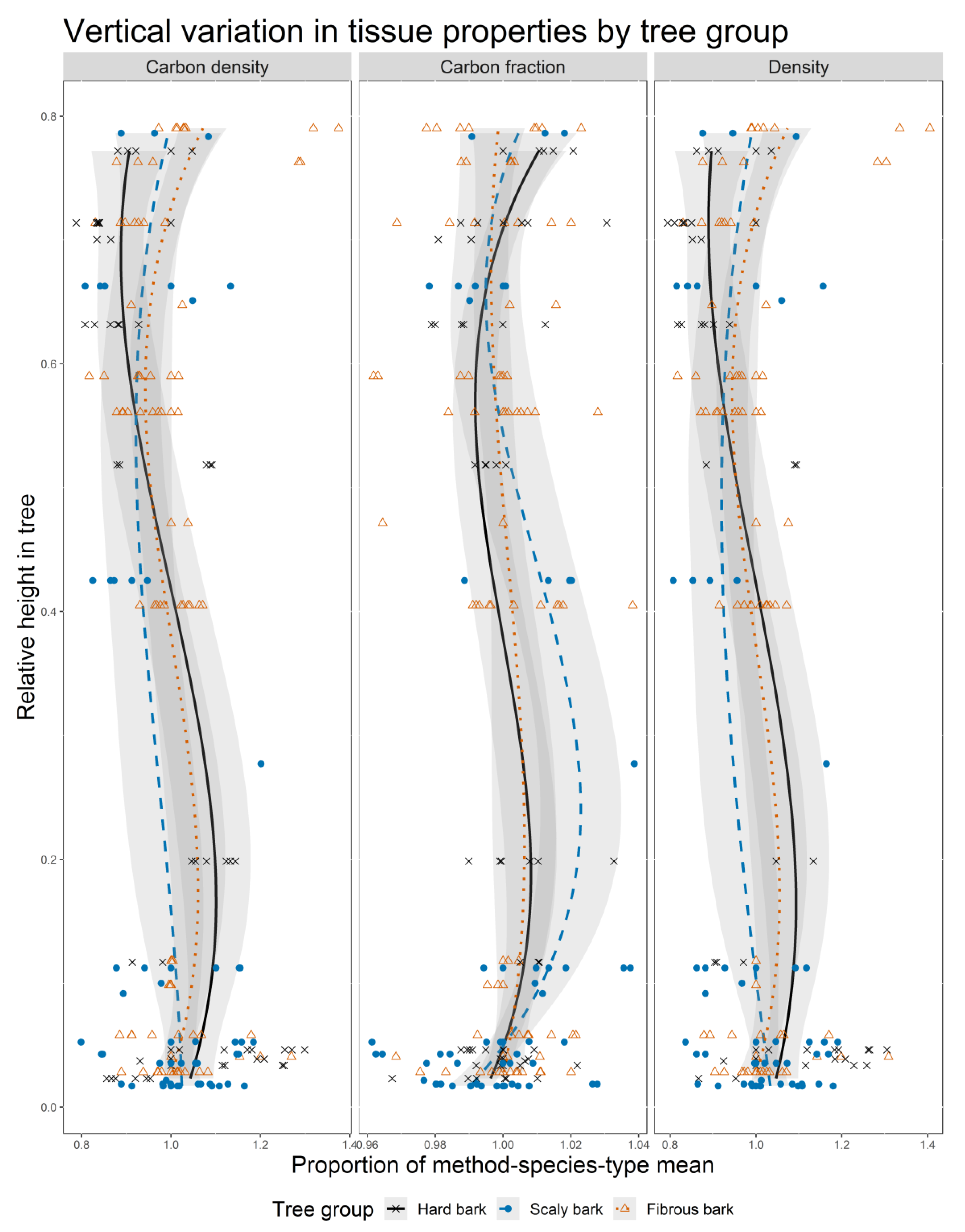
To look at vertical variation in tissue density properties between tree groups, B-splines were fit to each tree group with relative height as the predictor variable and percent mean deviation from the mean method-species-tissue type tissue property as the response. Using percent mean deviations from the method-species-tissue type centers the data and models the variations from these mean values to detect any vertical patterns in the data. The parameters of these B-spline models were compared using a Welch’s t-test and Bonferroni correction to determine if significant differences existed between parameters of the tree groups.

3. Results

Carbon fraction data is shown in

Table 2. Mean carbon fraction values, and coefficients of variation relative to an assumed carbon fraction of 0.5 (CV₅₀), for tissue types within nine conifer species. Standard deviations are shown in parenthesis after the mean carbon fraction and coefficient of variation values.

Species	Bark CF	% Bark CV50	Heartwood CF	% Heartwood CV50	Sapwood CF	% Sapwood CV50
Douglas-fir	0.588 (0.009)	17.6 (1.8)	0.513 (0.010)	2.6 (2.0)	0.510 (0.009)	2.0 (1.8)
Giant Sequoia	0.544 (0.004)	8.8 (0.8)	0.551 (0.010)	10.2 (2.0)	0.538 (0.010)	7.6 (2.0)
Incense-cedar	0.567 (0.015)	13.4 (3.0)	0.545 (0.009)	9.0 (1.8)	0.541 (0.008)	8.2 (1.6)
Jeffrey pine	0.515 (0.005)	3.0 (1.0)	0.539 (0.004)	7.8 (0.8)	0.513 (0.003)	2.6 (0.6)
Ponderosa pine	0.528 (0.008)	5.6 (1.6)	0.527 (0.008)	5.4 (1.6)	0.512 (0.005)	2.4 (1.0)
Red fir	0.528 (0.011)	5.6 (2.2)	0.533 (0.008)	6.6 (1.6)	0.511 (0.006)	2.2 (1.2)
Redwood	0.531 (0.013)	6.2 (2.6)	0.538 (0.012)	7.6 (2.4)	0.527 (0.007)	5.4 (1.4)
Sugar pine	0.570 (0.010)	14.0 (2.0)	0.534 (0.005)	6.8 (1.0)	0.532 (0.009)	6.4 (1.8)
White fir	0.525 (0.010)	5.0 (2.0)	0.517 (0.004)	3.4 (0.8)	0.507 (0.009)	1.4 (1.8)

. Measured mean tree tissue carbon fractions (CF_ij) and standard deviations, shown in parenthesis, ranged from 0.507 (0.009) for white fir sapwood to 0.588 (0.009) for Douglas-fir bark. Corresponding CV₅₀ values were 0.014 (0.018) to 0.176 (0.018). A comparison of carbon mass estimates for each species tissue type within 1000 kg example trees is shown in Figure S1. Bark (C_bm), sapwood (C_sm), and heartwood (C_hm) carbon masses were calculated using a carbon fraction of 0.5 for the standard approach example trees and using the CF_ij values from Table 2.

The mass of the example trees was set at 1000 kg, including bark, so that the only difference in carbon mass estimates within a species was due to the influence of using measured carbon fractions of the species-tissue types versus using the standard value of 0.5. Total carbon masses for the trees estimated with a 0.5 fraction were 500 kg. For the trees estimated using the CF_ij values from Table 2, the total carbon masses for each species are shown in

Table 3. Tree carbon masses and CV₅₀ values for each tree species studied based on applying measured CF values to example trees with a total biomass of 1000 kg.

Species	Carbon Mass (kg)	% CV50
Douglas-fir	519 (5)	3.80 (0.01)
Giant Sequoia	544 (5)	8.80 (0.01)
Incense-cedar	553 (6)	10.60 (0.01)
Jeffrey pine	529 (2)	5.80 (0.01)
Ponderosa pine	518 (4)	3.60 (0.01)
Red fir	522 (4)	4.40 (0.01)
Redwood	532 (6)	6.40 (0.01)
Sugar pine	541 (4)	8.20 (0.01)
White fir	518 (5)	3.60 (0.01)

, along with corresponding CV₅₀ estimates at the tree level. Tree carbon masses ranged from 518 kg for white fir to 553 kg for incense-cedar. CV₅₀ values ranged from 3.6% for white fir to 10.6% for incense-cedar (Table 3).

Symbols, descriptions, and units for covariates used in the final LME models are shown in

Table 4. Symbols, descriptions, and summary statistics of covariates found in final linear mixed effects (LME) models. Mean values are followed by corresponding standard deviations in parentheses.

Symbol	Covariate Descriptions	Mean	Units
CFijk	Average carbon fraction value for a given species tissue type and method	0.517 (0.019)	-
Dijk	Average oven-dry tissue density value for a given species tissue type	0.378 (0.068)	g/cm3
CDijk	Average carbon density value for a given species tissue type and method	0.195 (0.035)	g/cm3
p	Segment dry mass divided by segment green volume	0.378 (0.068)	g/cm3
RH	Height to core divided by total tree height	0.318 (0.294)	-
HLC	Height to live crown	14.2 (6.6)	m
FHLC	Height to core divided by HLC	0.813 (0.766)	-
HAR	Height to core divided by bole cross-sectional area at core height	0.013 (0.016)	m/cm2
LCR	Length of live crown divided by tree height	0.398 (0.151)	-
R	Radius to center of segment from pith	36.5 (51.0)	cm
RDb	Distance from bark divided by radius at core	0.313 (0.287)	-
RR	R divided by radius of bole at core height	0.687 (0.287)	-
Sa	Segment age	39.2 (46.8)	years

. Table 4 indicates that the most common types of covariate to be included in the final models were those related to height of sample in tree, crown length, or metrics related to height and crown length. Radial distance from pith and wood density also significantly improved final model fits, although they were not as consistent as covariates related to vertical position within the tree.

ANOVA results for comparisons of the nested models show that carbon fraction models were significantly improved with each increase in model complexity (

Table 5. ANOVA results for comparisons of nested tree property models. All models were regressed using maximum log-likelihood methods. Test column shows model numbers that were compared. The p-values result from log likelihood ratio tests for listed comparison. B_lX_l represents combinations of parameters and covariates fit to the model, CF is mean carbon fraction, D is mean tissue density, and CD is mean carbon density at a given model level. Nested model levels were: method (k), bark group (tk), species group (ik), species-tissue type groups (ijk). R_m² is the r-square value of the given model with fixed-effects only, while R_c² is the r-square value for the model with fixed and random-effects.

Covariates	DF	AIC	Model #	Test	p-Value	Rm2	Rc2
CFk	7	−1087	1	-	-	0.18	0.43
CFtk	15	−1093	2	1 vs. 2	<0.01	0.35	0.43
CFik	35	−1098	3	2 vs. 3	<0.01	0.47	0.47
CFik + BlXl	38	−1097	4	3 vs. 4	0.03	0.48	0.48
CFijk	82	−1274	5	4 vs. 5	<0.01	0.89	0.89
CFijk + BlXl	84	−1288	6	5 vs. 6	<0.01	0.89	0.90
Dk	7	−633	7	-	-	0.00	0.62
Dtk	15	−626	8	7 vs. 8	0.30	0.08	0.64
Dik	35	−616	9	8 vs. 9	0.08	0.36	0.65
Dik + BlXl	38	−638	10	9 vs. 10	<0.01	0.43	0.70
Dijk	81	−651	11	10 vs. 11	<0.01	0.54	0.86
Dijk + BlXl	85	−693	12	11 vs. 12	<0.01	0.56	0.90
CDk	7	−888	13	-	-	0.00	0.58
CDtk	15	−877	14	13 vs. 14	0.6874	0.05	0.60
CDik	35	−865	15	14 vs. 15	0.1204	0.34	0.62
CDik + BlXl	39	−892	16	15 vs. 16	<0.01	0.53	0.63
CDijk	81	−903	17	16 vs. 17	<0.01	0.56	0.87
CDijk + BlXl	85	−935	18	17 vs. 18	<0.01	0.64	0.88

). Accounting for tree group or tissue type alone did not significantly improve model performance for either density or carbon density. For density and carbon density models, significant improvements began at the species level with additional covariates added (Table 5). Models with tissue type and additional covariates (model #6, #12, and #18) performed significantly better than all other model forms for all three tree properties.

The final models for each tree property included covariates representing location of samples within trees (RH, R, HAR), and tree crown metrics (LCR, FHLC, HLC). Covariates related to tree size, such as diameter at breast height or tree height, were tested and not found to improve model fit (

Table 6. Summary of LME model parameter fits from Equation (2). X_l symbol descriptions can be found in Table 4. B_l is the matrix of parameter estimates for the given covariate matrix X_l. A p-value less than or equal to 0.05 indicates that the specified parameter estimate is significantly greater than zero. SE is the standard error of the parameter estimate shown in B_l. The % FV-upper and % FV-lower columns give the result of evaluating a given term at the mean covariate value from Table 4 plus one standard deviation (upper) or minus one standard deviation (lower) and then dividing by the mean response value.

Tissue Property	Xl	Bl	SE	p-Value	% FV-Upper	% FV-Lower
Carbon fraction	CFijk	1.0021	0.0018	<0.01	-	-
	p:FHLC	−0.0137	0.0046	0.04	−1.59	0.00
	HLC:FHLC	0.00033	0.00016	0.05	1.47	0.00
	HAR:HLC	−0.0146	0.0046	<0.01	−1.36	0.32
Density	Dijk	1.024	0.020	<0.01	-	-
	RH	−0.076	0.034	0.04	−12.24	−0.42
	RDb:Sa	0.0015	0.0003	<0.01	−1.50	11.44
	RDb:RR	−0.185	0.06	<0.01	−10.07	−0.03
Carbon density	CDijk	1.007	0.0201	<0.01	-	-
	FHLC:R	−0.00035	0.00016	0.03	−4.10	0.15
	RDb:RR	−0.0660	0.0327	0.04	−6.96	−1.99
	LCR:RH	−0.0847	0.0339	0.02	−11.96	0.11

). The carbon fraction model was significantly improved with the addition of an interaction term for tissue density and fraction of height to live crown (p:FHLC), while the density and carbon density models were both significantly improved with the addition of a term for the interaction between relative distance from bark and relative distance from center (RD_b:RR).

The potential influence of each term on the mean model estimate (CF_ijk, D_ijk, or CD_ijk) was demonstrated by the fraction of variation (FV) values in the FV-upper and FV-lower columns (Table 6). The upper fraction of variation was calculated by multiplying the given parameter estimate by the mean value of the term plus one standard deviation. The FV-lower values were determined by multiplying the parameter estimates by the mean value minus one standard deviation, then dividing both the FV-upper and FV-lower values by the mean model estimated value. The FV values were displayed as percentages of their respective mean tissue property values (CF_ijk, D_ijk, or CD_ijk). The FV values ranged from −12.24% to 11.44%, with the largest FV values found in the density and carbon density models.

B-spline fits showed vertical trends in each tree property (CF, D, CD) by tree bark group (Figure 1). There were significant differences between B-spline parameters for the three tree groups for each tree tissue property, thus indicating significant differences in the vertical trends between tree groups (

Table A1. Results for comparison of B-spline parameters fit to the three different tree groups for each tissue property. Comparisons are within tissue type only. Parameters with the same letter as a superscript for a given parameter are not significantly different from each other, while parameters between tree groups that have different letters are significantly different from each other. Int is the intercept of the spline fit; bs1, bs2, and bs3 are the parameter estimates for the first, second, and third knots, respectively. Parameter estimates within a tissue property are compared across bark groups with different superscript letters (a, b, or c) representing significant differences between bark groups for a given parameter (int compared to int, or bs 1 compared to bs1). Where superscripts are the same the differences were not significant.

	Parameter	Tissue Property
		Carbon	Density	Carbon Density
Furrowed bark	int	−0.0037 a	−0.0306 a	−0.0037 a
	bs 1	0.0399 a	0.4746 a	0.0399 a
	bs 2	−0.0381 a	−0.4065 a	−0.0381 a
	bs 3	0.0142 a	−0.1811 a	0.0142 a
Fibrous bark	int	0.0003 b	0.0003 b	0.0003 b
	bs 1	0.0182 b	0.1937 b	0.0182 b
	bs 2	−0.0117 a	−0.2562 a	−0.0117 a
	bs 3	−0.0017 a	0.0745 a	−0.0017 a
Scaly bark	int	−0.0093 c	−0.0093 c	−0.0093 c
	bs 1	0.0846 c	0.0846 c	0.0846 c
	bs 2	−0.0335 b	−0.0335 b	−0.0335 b
	bs 3	0.0148 b	0.0148 b	0.0148 b

). The values on the x-axis are expressed as percentages of species-tissue type values to center the data. This allowed for a more meaningful comparison of deviations from the average for each tree group. Density and carbon density showed the greatest range in deviations from the species-tissue type means, ranging from approximately 0.8 to 1.4, while carbon fractions stayed relatively close to their respective means, ranging from 0.96 to 1.04. Density and carbon fraction showed negative correlations in their trends with significant variation between tree groups. The fibrous bark group displayed the greatest range in deviations from the mean, followed by the furrowed bark group, with the scaly bark group displaying less variation.

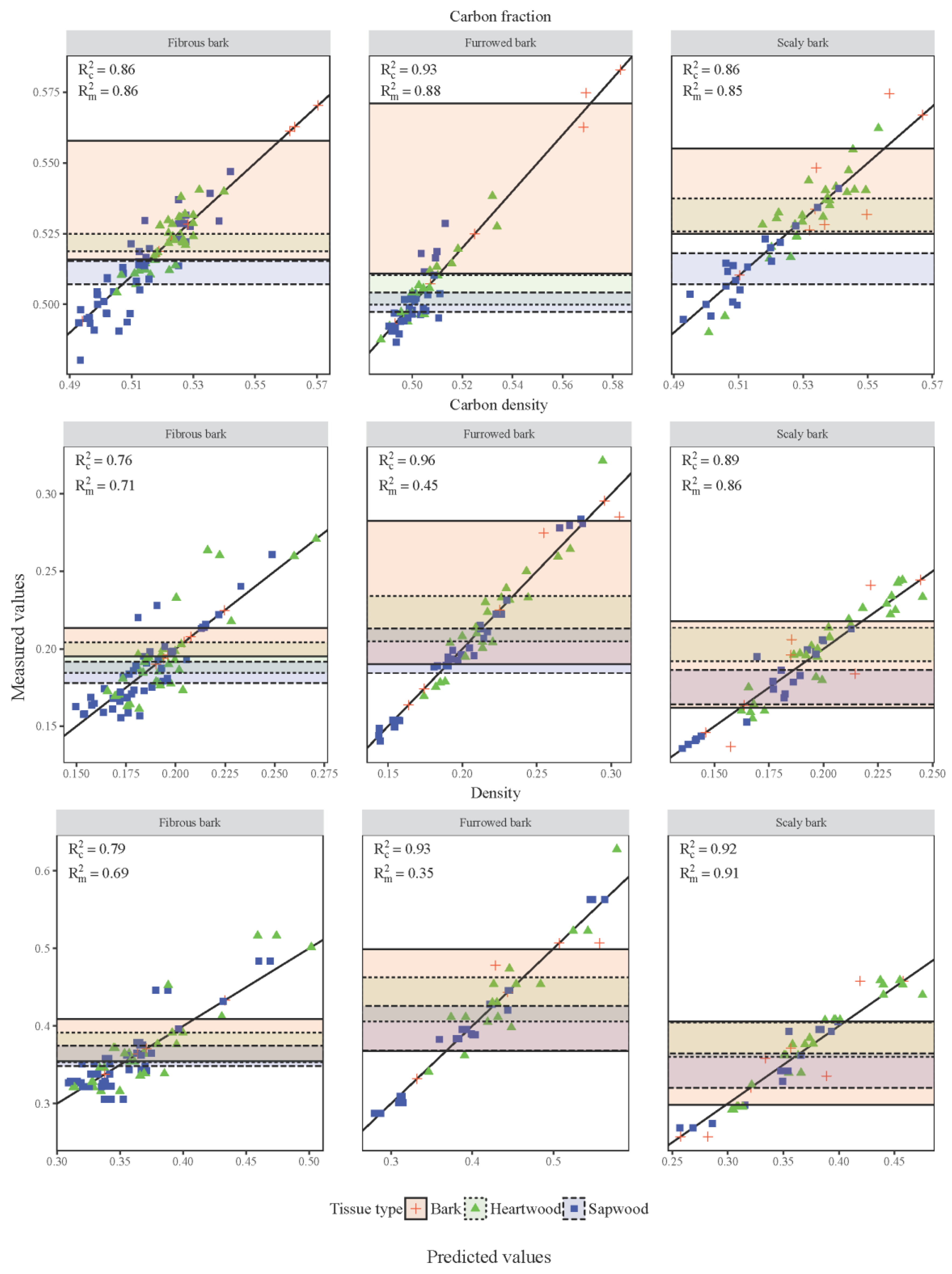
The shaded regions in the graph of the predictions from the LME model versus observed data (Figure 2) represent the 95% confidence intervals for each tissue type within a given bark group tissue property. The lack of overlapping confidence intervals between the heartwood samples of the three tree groups, along with the lack of overlapping confidence intervals for the sapwood portion of the furrowed bark group and the other two groups, indicated significant differences between those means across the tree groups. The wide confidence intervals for the bark portions of the graphs were related to the high variation found in the bark samples. The R_c² values for the model fits ranged from 0.64 to 0.95, while the R_m² values ranged from 0.34 to 0.91. The difference in these two values indicated the variation in the model that is explained by the random effects related to individual trees, and individual cores taken from those trees. Differences between the R_m² and R_c² were most pronounced in the density properties of the furrowed bark trees, with smaller differences displayed by carbon density compared to the wood density.

4. Discussion

4.1. Measured Carbon Fractions versus the 0.5 Value

The differences between carbon mass estimates derived from measured CF_ij values versus the values derived from assuming a carbon fraction of 0.5 (Figure S1) demonstrate the importance of accurately accounting for variation in carbon fractions within trees and between tree species. The increase in estimated carbon mass related to using CF_ij values ranged from 3.6% to 10.6%, which represents the error associated with assuming that all wood biomass has a carbon fraction of 0.5. Given that average carbon fractions for angiosperms are lower than 0.5 [29], conifers almost certainly play a more important role in global carbon cycles than global estimates based on the 0.5 value currently suggest.

The difference in carbon mass estimates of tissue types are equally important, as different tissues store carbon for variable amounts of time [49]. Different tissue decay rates mean different rates of carbon dioxide release from the separate tissue carbon pools. Correctly estimating these pools is an important first step in improving the overall understanding of carbon decay dynamics in forests. Accounting for these differences is also important to accurately track carbon mass in forest products.

4.2. Comparisons between Model Complexity Levels

The improvement in AIC and the significant difference determined through log-likelihood ratios shown between model 1 and model 2 (Table 5) demonstrates the potential to partially explain the variation in carbon fraction values with easily observed bark characteristics. One measure of the improvement in carbon fraction estimation by grouping trees by bark characteristics is the improvement in R_m² from 0.18 to 0.35, nearly doubling the explained variation due to tree grouping. There is no improvement in model performance for either density or carbon density at the tree group level. This is partially due to the high variation found in these two properties between individuals within a species and within individual trees, as shown by the difference in R_c² and R_m² values in Figure 2.

The higher AIC for the species average carbon density model (CD_ik) compared to the species-tissue type model (CD_ijk) (Table 5) provides interesting insights into the importance of estimating tissue-level carbon fractions and densities in different species. Tissue types from the same species can have different average carbon fractions [27,28,32] and different average densities [50]: accounting for these known differences in any carbon density model should improve the predictive power of the model. Interestingly, the species average level model (CD_ik) does not appear to improve model performance above the CD_k model, suggesting that studies into carbon density should focus on a level of complexity at least as complex as the tissue level in order to achieve meaningful improvements in carbon density estimates.

4.3. Carbon Fraction Modeling

Carbon mass estimates using a value of 0.5 often include no error term for the estimate, implying that the term itself has no error. Measured CV₅₀ values as high as 17.6% (Table 2) indicate this assumption is incorrect for both whole tree carbon mass and tree tissue carbon mass. There is a strong indication that conifer carbon fractions are generally higher than 0.5 and that angiosperms are generally lower than 0.5 [29,36]. Our data support this finding, as all conifer tissues measured in our study had carbon fractions higher than 0.5. This suggests caution should be taken when estimating representative conifer and hardwood carbon fractions for regional carbon estimates.

Though we did not study angiosperms, our findings of significant differences between tissue types within species are consistent with the findings of studies that have specifically looked at carbon fractions in different angiosperm tissue types [26,35,51]. The majority of studies on carbon fraction, however, have not studied different tissue types within a species as potential sources of variation. This is especially true for angiosperm species where sapwood has been the primary tissue type studied [29]. Given the potential for significantly different carbon fractions between wood types, it is advisable to study both heartwood and sapwood in developing representative tree stem carbon fraction values. This could have important consequences for global carbon storage estimates. It is important to note that whole tree cores are not representative of the entire tree stem at the point of extraction, as the tissue masses in the cores are not proportional to their biomass balance in the stem. Therefore, we suggest that cores be used to estimate the separate tree tissues for carbon fractions and those results be applied to biomass component models that accurately estimate the separate biomasses of the tree components.

The improvement in carbon fraction model fit with increasing model complexity shown in Table 5 demonstrates that accounting only for species average values does not accurately estimate the carbon fractions found within trees, though species-level averages are clearly superior to using a value of 0.5. This finding is consistent with other studies that have documented significant variation between sapwood, heartwood, and bark within conifers [27,28,31,38]. In a review of existing carbon fraction studies, Thomas and Martin [29] found only six studies that measured carbon fractions for different bole tree tissues and none of those studies looked at carbon fractions as measured by all of the common methodologies. By including all of the common carbon fraction analysis methods represented by the Thomas and Martin data [30], our results are more broadly applicable to carbon fraction research as a whole without being overly influenced by any one method.

The significant improvement in model performance with the addition of the parameter covariate matrix B_lX_l (model #4 and #6) indicates considerable potential to more accurately predict carbon fractions by utilizing measurable tree characteristics. Our best-fit carbon fraction model (model #6), which included the B_lX_l matrix, demonstrates that in addition to tissue type, including covariates related to crown length and relative position within the tree result in more accurate carbon fraction estimates. Model #4 did not outperform the more complex models, which suggests that significant physiological differences between tissue types are driving the relationship.

The significant negative relationship between CF_ijk and the p:FHLC interaction term (Table 6) has not been identified in previous studies. This term has the potential to shift the mean model estimate by up to −1.59% and indicates important differences in carbon fractions between the top and bottom of the tree crown. Bert and Danjon [32] found a quadratic relationship between carbon fraction and relative tree height but did not report such a relationship for relative position within the crown, as found in this study. The negative relationship found in our study suggests a reduction in carbon fraction within tissue types with increasing relative position in the tree crown. This negative relationship with relative crown position is increased for denser tissue samples (higher p average) within a given species-tissue type. Wood density can be lower in wood found above the base of the live crown [21] for some species, which would lead to a decrease in the negative impact from the p:FHLC term for those species. The negative correlation between carbon fraction and tissue density is most easily seen in the fibrous and furrowed bark tree groups in Figure 1, as the carbon and density curves for those groups are nearly mirror images of each other. It is possible that, in isolation, the effect of the p:FHLC term would be very similar to the quadratic relationship found by Bert and Danjon [32], depending on where peak density occurs in a tree crown. The significant improvement in carbon fraction estimation between model #1 and #2, and the lack of overlap in confidence intervals between mean tissue type values in Figure 2, indicates that grouping these trees by bark characteristic could be a reasonable first step in improving carbon fraction estimates. The improvement in carbon fraction estimation by accounting for bark features (Table 5) could be beneficial for carbon estimation in tropical forests, where measuring carbon fractions for every species can be impractical. In these cases, improving carbon fraction estimates by grouping species using easily observed bark characteristics could be beneficial by allowing for improved carbon estimation without the costly process of measuring every species present for carbon fractions.

The positive parameter estimate for the HLC:FHLC term indicates an increased carbon fraction for tissues in trees with high HLC values. This term has the potential to shift the mean model estimate up to 1.47%, depending on the size of the tree and the position relative to the live crown. This increase in carbon fraction is greater for tree tissues located above the live crown. Given this relationship, tall trees with high height to live crowns would be expected to have higher overall average carbon fraction values than short trees with small height to live crowns. This relationship could indicate the potential for canopy class to influence carbon fractions, as all else being equal dominant trees will have longer live crowns than suppressed trees, thus leading to higher FHLC values for dominant trees and therefore a larger positive effect of the HLC:FHLC term.

The negative parameter estimate for the HAR:HLC term indicates a reduction of carbon fraction at the top of the tree, with a rapid weakening of this relationship with increasing distance from the tree top. This term has the smallest potential impact, ranging between −0.47% to 0%. This is because the HAR term decreases at a faster rate than does distance from the tree top. A rapidly decreasing HAR term and a constant HLC term results in a stronger negative relationship near the top of trees than exists further down, though with an overall strengthening of the relationship with increasing HLC values. This negative trend toward the top of trees is primarily displayed by the fibrous bark group from an RH value of 0.4 to 1.0, and may act to bring predicted carbon values back toward the mean species-tissue type value (Figure 1).

The mean species-tissue type carbon fraction parameter estimate (CF_ijk) of 1.002 (0.002), suggests that observed carbon fractions are evenly distributed around the mean species-tissue type carbon fraction values. If the parameter estimate was not equal to one, it could indicate that the variance might be better explained by additional covariates or that the variance was not equally distributed around the mean value.

The modeled relationships showed little improvement with the addition of random effects, as shown by the small differences between R_c² and R_m² values in Figure 2. This indicates that the fixed effect portions of the models, specifically the species-specific tissue type averages and the covariate matrix, are accounting for the majority of the variation in the data. This is a critical point in understanding carbon fractions because it indicates that most of the variation in carbon fraction in conifers can be accounted for by calculating species-tissue type averages. This approach may be infeasible in areas with high species diversity, however, in those cases grouping trees by bark characteristics could lead to some improvements in carbon fraction estimation similar to the improvement found between models #1 and #2.

4.4. Tissue Density

Wood density has been studied for varying purposes for over a century [15,52]. Appropriate application of this historical data to carbon mass estimation requires an understanding of the underlying relationships between carbon fraction and tissue density. The lack of improvement in AIC in comparing model #7 with models #8 and #9 (Table 5) indicates that partitioning tree density in tree group and species-level categories alone does not significantly improve model estimates. The best tissue density model utilized tissue type averages and additional covariates (model #12). This means that accounting for changes in tissue density related to observable tree characteristics in addition to tissue type averages not only results in a significant difference in log-likelihood ratios but also improves overall model AIC relative to any of the means only models (D_k, D_ik, D_ijk).

In this study, the final density model (Table 6) estimates a negative parameter associated with RH, a phenomenon that is common among conifers [21]. This interaction between RH and D_ijk is likely driven by the tree species in the furrowed bark group, which show the largest reduction in density with increasing RH values (Figure 1). The potential for this term to influence the mean model estimate is large, ranging from between 12.24% to −0.42%. This indicates the potential improvement in model fit that could be obtained by accounting for the relative position of tissues within the tree.

The reduction in predicted density is partially balanced by the positive parameter estimate for the RD_b:S_a interaction term. The impact from this term ranges from −1.50% to 11.44%, nearly equal to the negative range of values from the RH term. The RD_b:S_a term indicates that older tissues closer to the pith have higher density values on average. This may be due to increasing lignification that occurs in older tissues, and the accumulation in extractive materials in some tissues over time.

The negative parameter estimate for the RD_b:RR term is best interpreted as creating a maximum response at the center of a core with decreasing values away from that core center. Overall, the potential impact on the mean model estimate ranges from this term is −10.07% to −0.03%, which is a large amount of potential variation related to one term.

As with the carbon fraction model, the term representing the species-tissue type average values (D_ijk) had a parameter estimate statistically indistinguishable from 1 (Table 6). This indicates that the data were fairly evenly distributed around the mean values. The overall fit of the model to the data was significantly improved with the inclusion of random effects related to individual trees and cores (Figure 2). This is a result of the large inter- and intra-tree variability in wood density. Although the addition of the parameter matrix improved the fit of the model to the data, significant improvement in the model fit was due to the inclusion of random effects, indicating that the fixed effects are not describing as much of the variability as they are in the case of carbon fractions (Table 5). This could be remedied by adding variables that account for ring width, proportion of earlywood to latewood, and other tree ring-specific variables, as those have been shown to be closely correlated with wood density [53]. However, these ring-specific variables are not easily measured, and therefore not very useful in estimating overall tree biomass or carbon mass without time consuming sampling procedures.

4.5. Carbon Density

This study used paired density and carbon fraction samples in order to directly analyze the relationship between these two tree properties. The product of these values is carbon density, and, as can be seen in Figure 1, density dominates the resulting relationship. The trend lines in the carbon density graph are somewhat less extreme versions of the corresponding density curves, with each carbon density curve remaining closer to the mean species-tissue type value at a given RH value than either the carbon fraction or tissue density curves. This reduced spread around the mean values is due to the negative relationships between carbon fraction and tissue density. The trend in carbon density has the same shape as the density curves due to the much larger variation within density samples compared to the carbon fraction samples. Given the complexity of the relationship between carbon fraction and tissue density, it would be advisable to study these two tree characteristics with paired samples rather than trying to study them as independent variables and then later multiply the resulting values together.

The negative parameter for the FHLC:R term indicates a reduction in carbon density closer to the pith and higher in the crown. This reduction is more significant for large diameter trees and would be applicable to each species-tissue type. This effect could partially be driven by the presence of large old-growth trees in the study, such as giant sequoia and some individual pines. It seems that it is this trend in density that is driving the trend in carbon density, as the carbon fraction model suggests no significant effect related to distance from pith, while the density model has negative relationships for relative height and relative distance from the bark.

The negative parameter estimate for the RD_b:RR term suggests low carbon density values near pith and values that increase radially from the pith. This is likely driven by the same relationship in the density model, as no comparable term was found for the carbon fraction model.

The LCR:RH term suggests decreasing carbon density for trees with greater live crown proportions, with a decreasing trend up the tree. This term reflects crown relationships that are prevalent in the carbon fraction model, as well as relative height relationships in the density model. It may also indicate that trees with greater live crown ratios will have larger proportions of crown wood, which can be lower in density than wood formed below the crown. This is consistent with our understanding of juvenile and mature wood formation in conifers [54].

The even distribution of the values around the mean is indicated by the mean estimate parameter value of 1.007 (Table 6). This suggests that the variables in the model are reflecting the trends in both density and carbon fraction in a balanced way.

The best-fit models for carbon density are less influenced by the addition of random effects (smaller range in R_c² and R_m² values for most tree groups) than the tissue density models but more than the carbon fraction models (Figure 2). As carbon density is a combination of tissue density and carbon fraction, it is logical that the high variability displayed by the density samples would be somewhat reduced by the lower residual variance found in the carbon fraction values. It is also likely that the negative correlation between carbon fraction and tissue density are partially responsible for reducing the residual error allocated to the random effects. This finding is promising, as the high variability in tissue density creates high variability in any final biomass or carbon mass estimate; however, if that variability can be partially offset by correctly accounting for carbon fraction values then the overall carbon mass estimate would display reduced error relative to biomass estimates.

5. Conclusions

Our study found significant differences in measured carbon fraction values from the widely used value of 0.5 for different tissue types and for whole trees using nine western North American conifer species. Deviations in measured carbon fractions from this value were as high as 17.6%. Applying measured carbon fractions to biomass data resulted in estimates of whole tree bole carbon masses up to 10.6% higher than estimates that used a 0.5 carbon fraction. Our study determined that significant improvements in carbon mass estimation in conifer trees are possible by modeling carbon using species-tissue type averages and their relationships with measurable tree characteristics related to position in tree and crown characteristics. Some improvement in carbon fraction modeling occurred by grouping tree species by visible bark characteristics, thus demonstrating the potential to simplify carbon estimates in forests with high tree species diversity. The negative relationship between tissue density and carbon fraction observed in this study demonstrated why simple approaches to converting biomass into carbon are flawed. Additionally, this relationship suggests that these two key tree properties—average carbon and average density—should be studied using a paired sample approach to determine possible relationships between the two properties, as that understanding can improve carbon mass estimates.

References

- Brown, S. Measuring carbon in forests: Current status and future challenges. Environ. Pollut. 2002, 116, 363–372. [Google Scholar] [CrossRef]
- Fogel, R.; Cromack, K. Effect of habitat and substrate quality on Douglas-fir litter decomposition in Western Oregon. Can. J. Bot. 1977, 55, 1632–1640. [Google Scholar] [CrossRef]
- Johansson, M.B.; Berg, B.; Meentemeyer, V. Litter mass-loss rates in late stages of decomposition in a climatic transect of pine forests. Long-term decomposition in a Scots pine forest. IX. Can. J. Bot. 1995, 73, 1509–1521. [Google Scholar] [CrossRef]
- Dixon, R.K.; Brown, S.; Houghton, R.A.; Solomon, A.M.; Trexier, M.C.; Wisniewski, J. Carbon pools and flux of global forest ecosystems. Science 1994, 263, 185–190. [Google Scholar] [CrossRef] [PubMed]
- Goodale, C.L.; Apps, M.J.; Birdsey, R.A.; Field, C.B.; Heath, L.S.; Houghton, R.A.; Jenkins, J.C.; Kohlmaier, G.H.; Kurz, W.; Liu, S.; et al. Forest Carbon Sinks in the Northern Hemisphere. Ecol. Appl. 2002, 12, 891–899. [Google Scholar] [CrossRef]
- Jenkins, J.C.; Chojnacky, D.C.; Heath, L.S.; Birdsey, R.A. National-Scale Biomass Estimators for United States Tree Species. For. Sci. 2003, 49, 12–35. [Google Scholar]
- Chojnacky, D.C.; Heath, L.S.; Jenkins, J.C. Updated generalized biomass equations for North American tree species. Forestry 2014, 87, 129–151. [Google Scholar] [CrossRef]
- Karchesy, J.; Koch, P. Energy Production from Hardwoods Growing on Southern Pine Sites; General Technical Report SO-24; U.S. Department of Agriculture, Forest Service, Southern Forest Experiment Station: Pineville, Louisiana, DC, USA, 1979; pp. 1–63.
- Harmon, M.E.; Ferrell, W.K.; Franklin, J.F. Effects on Carbon Storage of Conversion of Old-Growth Forests to Young Forests. Science 1990, 247, 699–702. [Google Scholar] [CrossRef] [PubMed]
- Dewar, R.C.; Cannell, M.G.R. Carbon sequestration in the trees, products and soils of forest plantations—An analysis using UK examples. Tree Physiol. 1992, 11, 49–71. [Google Scholar] [CrossRef] [PubMed]
- Hollinger, D.Y.Y.; MacLaren, J.P.P.; Beets, P.N.N.; Turland, J. Carbon sequestration by New Zealand’s plantation forests. New Zeal. J. For. Sci. 1993, 23, 194–208. [Google Scholar]
- Matthews, G. The Carbon Content of Trees; Forestry Commission Technical Paper 4; Forestry Commission: Edinburgh, Scotland, UK, 1993.
- Thuille, A.; Buchmann, N.; Schulze, E.D. Carbon stocks and soil respiration rates during deforestation, grassland use and subsequent Norway spruce afforestation in the Southern Alps, Italy. Tree Physiol. 2000, 20, 849–857. [Google Scholar] [CrossRef] [PubMed]
- Pacala, S.W.; Hurtt, G.C.; Baker, D.; Peylin, P.; Houghton, R.A.; Birdsey, R.A.; Heath, L.; Sundquist, E.T.; Stallard, R.F.; Ciais, P.; et al. Consistent land- and atmosphere-based U.S. carbon sink estimates. Science 2001, 292, 2316–2320. [Google Scholar] [CrossRef] [PubMed]
- Chave, J.; Andalo, C.; Brown, S.; Cairns, M.A.; Chambers, J.Q.; Eamus, D.; Fölster, H.; Fromard, F.; Higuchi, N.; Kira, T.; et al. Tree Allometry and Improved Estimation of Carbon Stocks and Balance in Tropical Forests. Oecologia 2005, 145, 87–99. [Google Scholar] [CrossRef] [PubMed]
- Woodbury, P.B.; Smith, J.E.; Heath, L.S. Carbon sequestration in the U.S. forest sector from 1990 to 2010. For. Ecol. Manag. 2007, 241, 14–27. [Google Scholar] [CrossRef]
- Fahey, T.J.; Woodbury, P.B.; Battles, J.J.; Goodale, C.L.; Hamburg, S.; Ollinger, S.; Woodall, C.W. Forest carbon storage: Ecology, management, and policy. Front. Ecol. Environ. 2010, 8, 245–252. [Google Scholar] [CrossRef]
- Van Deusen, P.; Roesch, F.A. Sampling a tree for Total Volume, Biomass, and Carbon. J. For. 2011, 109, 131–135. [Google Scholar]
- Woodall, C.W.; Heath, L.S.; Domke, G.M.; Nichols, M.C. Methods and Equations for Estimating Aboveground Volume, Biomass, and Carbon for Trees in the U.S. Forest Inventory; General Technical Report NRS-88; U.S. Department of Agriculture, Forest Service, Northern Research Station: Newtown Square, PA, USA, 2010.
- Nogueira, E.M.; Fearnside, P.M.; Nelson, B.W.; Barbosa, R.I.; Keizer, E.W.H. Estimates of forest biomass in the Brazilian Amazon: New allometric equations and adjustments to biomass from wood-volume inventories. For. Ecol. Manag. 2008, 256, 1853–1867. [Google Scholar] [CrossRef]
- Chave, J.; Coomes, D.; Jansen, S.; Lewis, S.L.; Swenson, N.G.; Zanne, A.E. Towards a worldwide wood economics spectrum. Ecol. Lett. 2009, 12, 351–366. [Google Scholar] [CrossRef] [PubMed] [Green Version]
- Nogueira, E.M.; Fearnside, P.M.; Nelson, B.W.; Franca, M.B. Wood density in forests of Brazil’s ‘arc of deforestation’: Implications for biomass and flux of carbon from land-use change in Amazonia. For. Ecol. Manag. 2007, 248, 119–135. [Google Scholar] [CrossRef]
- Wiemann, M.C.; Williamson, G.B. Radial Gradients in the Specific Gravity of Wood in Some Tropical and Temperate Trees. For. Sci. 1989, 35, 197–210. [Google Scholar]
- Woodcock, D.W.; Shier, A.D. Wood specific gravity and its radial variations: The many ways to make a tree. Trees 2002, 16, 437–443. [Google Scholar] [CrossRef]
- Lamlom, S.H.; Savidge, R.A. A reassessment of carbon content in wood: variation within and between 41 North American species. Biomass Bioenerg. 2003, 25, 381–388. [Google Scholar] [CrossRef]
- Lamlom, S.H.; Savidge, R.A. Carbon content variation in boles of mature sugar maple and giant sequoia. Tree Physiol. 2006, 26, 459–468. [Google Scholar] [CrossRef] [PubMed] [Green Version]
- Jones, D.A.; O’Hara, K.L. Carbon density in managed coast redwood stands: Implications for forest carbon estimation. Forestry 2012, 85, 99–110. [Google Scholar] [CrossRef]
- Jones, D.A.; O’Hara, K.L. The influence of preparation method on measured carbon fractions in tree tissues. Tree Physiol. 2016, 36, 1177–1189. [Google Scholar] [CrossRef] [PubMed] [Green Version]
- Thomas, S.C.; Martin, A.R. Carbon Content of Tree Tissues: A Synthesis. Forests 2012, 3, 332–352. [Google Scholar] [CrossRef] [Green Version]
- Thomas, S.C.; Martin, A.R. Data from: Carbon content of tree tissues: A synthesis. Forests 2012. [Google Scholar] [CrossRef]
- De Aza, C.H.; Turrión, M.B.; Pando, V.; Bravo, F. Carbon in heartwood, sapwood and bark along the stem profile in three Mediterranean Pinus species. Ann. For. Sci. 2011, 68, 1067–1076. [Google Scholar] [CrossRef] [Green Version]
- Bert, D.; Danjon, F. Carbon concentration variations in the roots, stem and crown of mature Pinus pinaster (Ait.). For. Ecol. Manag. 2006, 222, 279–295. [Google Scholar] [CrossRef]
- Gao, B.; Taylor, A.R.; Chen, H.Y.H.; Wang, J. Variation in total and volatile carbon concentration among the major tree species of the boreal forest. For. Ecol. Manag. 2016, 375, 191–199. [Google Scholar] [CrossRef]
- Jones, D.A.; O’Hara, K.L.; Battles, J.J.; Gersonde, R.F. Leaf Area Prediction Using Three Alternative Sampling Methods for Seven Sierra Nevada Conifer Species. Forests 2015, 6, 2631–2654. [Google Scholar] [CrossRef] [Green Version]
- Castaño-Santamaría, J.; Bravo, F. Variation in carbon concentration and basic density along stems of sessile oak (Quercus petraea (Matt.) Liebl.) and Pyrenean oak (Quercus pyrenaica Willd.) in the Cantabrian Range (NW Spain). Ann. For. Sci. 2012, 69, 663–672. [Google Scholar] [CrossRef]
- Ma, S.; He, F.; Tian, D.; Zou, D.; Yan, Z.; Yang, Y.; Zhou, T.; Huang, K.; Shen, H.; Fang, J. Variations and determinants of carbon content in plants: A global synthesis. Biogeosci. Discuss. 2017, 1–22. [Google Scholar] [CrossRef]
- Martin, A.R.; Thomas, S.C.; Zhao, Y. Size-dependent changes in wood chemical traits: A comparison of neotropical saplings and large trees. AoB Plants 2013, 5, 1–14. [Google Scholar] [CrossRef]
- Correia, A.C.; Tomé, M.; Carlos, P.; Sónia, F. Biomass allometry and carbon factors for a Mediterranean pine (Pinus pinea L.) in Portugal. For. Syst. 2010, 19, 418–433. [Google Scholar] [CrossRef]
- Poorter, L.; Mcneil, A.; Hurtado, V.H.; Prins, H.H.T.; Putz, F.E. Bark traits and life-history strategies of tropical dry- and moist forest trees. Funct. Ecol. 2014, 28, 232–242. [Google Scholar] [CrossRef]
- Melson, S.; Harmon, M. Estimates of live-tree carbon stores in the Pacific Northwest are sensitive to model selection. Carbon Balance Manag. 2011, 6, 2. [Google Scholar] [CrossRef] [PubMed] [Green Version]
- Means, J.E.; Hansen, H.A.; Koerper, G.J.; Alaback, P.B.; Klopsch, M.W. Software for Computing Plant Biomass—BIOPAK Users Guide; General Techcal Report PNW-GTR-340; U.S. Department of Agriculture, Forest Service, Pacific Northwest Research Station: Portland, OR, USA, 1994; p. 184.
- Calcagno, V. Glmulti: Model Selection and Multimodel Inference Made Easy; R Package Version 1.7; R Core Team: Vienna, Austria, 2013; Volume 1, p. 67. Available online: https://rdrr.io/cran/glmulti/ (accessed on 10 June 2015).
- Team, R.C. R: A Language and Environment for Statistical Computing; R Foundation for Statistical Computing: Vienna, Austria, 2018; Available online: https://www.R-project.org/ (accessed on 23 April 2017).
- Pinheiro, J.; Bates, D.; DebRoy, S.; Sarkar, D.; Team, R.C. nlme: Linear and Nonlinear Mixed Effects Models; R Package Version 3.1-137; R Core Team: Vienna, Austria, 2007; pp. 31–128. Available online: https://rdrr.io/cran/nlme/ (accessed on 15 May 2015).
- Zuur, A.F.; Ieno, E.N.; Elphick, C.S. A protocol for data exploration to avoid common statistical problems. Methods Ecol. Evol. 2010, 1, 3–14. [Google Scholar] [CrossRef]
- Pinheiro, J.C.; Bates, D.M. Mixed-Effects Models in S and S-Plus; Chambers, J., Eddy, W., Härdle, W., Sheather, S., Tierney, L., Eds.; Springer Inc.: New York, NY, USA, 2000; ISBN 0-387-98957-9. [Google Scholar]
- Akaike, H. A new look at the statistical model identification. IEEE Trans. Automat. Contr. 1974, 19, 716–723. [Google Scholar] [CrossRef]
- Nakagawa, S.; Schielzeth, H. A general and simple method for obtaining R2 from generalized linear mixed-effects models. Methods Ecol. Evol. 2013, 4, 133–142. [Google Scholar] [CrossRef]
- Van Geffen, K.G.; Poorter, L.; Sass-Klaassen, U.; van Logtestijn, R.S.P.; Cornelissen, J.H.C. The trait contribution to wood decomposition rates of 15 Neotropical tree species. Ecology 2010, 91, 3686–3697. [Google Scholar] [CrossRef] [PubMed]
- Miles, P.D.; Smith, W.B. Specific Gravity and other Properties of Wood and Bark for 156 Tree Species Found in North America; U.S. Department of Agriculture, Forest Service, Northern Research Station: Newtown Square, PA, USA, 2009.
- Peri, P.L.; Gargaglione, V.; Martínez Pastur, G.; Lencinas, M.V. Carbon accumulation along a stand development sequence of Nothofagus antarctica forests across a gradient in site quality in Southern Patagonia. For. Ecol. Manag. 2010, 260, 229–237. [Google Scholar] [CrossRef]
- Stamm, A.J. Density of wood substance, adsorption by wood, and permeability of wood. J. Phys. Chem. 1928, 33, 398–414. [Google Scholar] [CrossRef]
- Peng, M.; Stewart, J. Development, validation, and application of a model of intra-and inter-tree variability of wood density for lodgepole pine in western Canada. Can. J. For. Res. 2013, 43, 1172–1180. [Google Scholar] [CrossRef]
- Zobel, B.J.; Sprague, J.R. Juvenile Wood in Forest Trees; Timell, T.E., Ed.; Springer Series in Wood Science; Springer: Berlin, Germany, 1998. [Google Scholar]
Figure 1.
Fractions of species-tissue type averages across relative heights are shown. Species values are grouped into three bark characteristic categories: fibrous, scaly, and furrowed. LOESS regressions are shown for each tree group to demonstrate the moving average change in tree property throughout the tree bole.
Figure 2.
Measured values for carbon fraction, tissue density, and carbon density are shown relative to predicted values from the best-fit LME models from Table 6. Rc2 values correspond to the proportion of variance explained by the fixed and random effects in the model, while Rm2 values correspond to variance explained by the fixed effects alone. Data is grouped by bark characteristics and tissue types are differentiated by shapes and color. Shaded regions represent the 95% confidence interval in measured values for a given tissue type within a particular tree group.