Pedunculate and Sessile Mixed Oak Forest Regeneration Process in Lithuania

1
Forest Genetics and Tree Breeding Department, Institute of Forestry, Lithuanian Research Centre for Agriculture and Forestry, Liepų str. 1, LT-53101 Girionys, Kaunas District, Lithuania
2
Institute of Forest Biology and Silviculture, Aleksandras Stulginskis University, Studentų str. 11, LT-53361 Akademija, Kaunas District, Lithuania
*
Author to whom correspondence should be addressed.
Forests 2018, 9(8), 459; https://doi.org/10.3390/f9080459
Submission received: 4 July 2018
/
Revised: 20 July 2018
/
Accepted: 25 July 2018
/
Published: 27 July 2018
(This article belongs to the Section Forest Ecology and Management)
Abstract
:Pedunculate and sessile oak species are sympatric. These oaks hybridize with one another, and this process influences the development of undergrowth. The purpose of this study was to determine how different oak species influence the forest regeneration process. For this purpose, the forest was divided into eight transects of 300 m and 100 m widths, distinguished into temporary plots of 10 m in diameter covering the whole territory of the forest. The distribution of oak undergrowth was calculated by four oak height groups, determining the composition of the first storey, covering of underbrush and herbaceous plant, and forest site. We determined that the spread of oak differed depending on the first storey tree species and underbrush. Grass cover was the biggest influence on the sessile oak. The impurity of sessile oak in oak stands had a positive impact on the development of undergrowth, since the entire undergrowth develops faster than separate components of the undergrowth.
1. Introduction
Forest succession is a slow process and may be interrupted by natural and cultural disturbances in the landscape [1,2,3] For each plant, tree or their group, it can be viewed as a complex biological system component having the specific structure, function and features that interact with the environment to carry out specific functions. The undergrowth plays an important role in stands of natural regeneration processes [4]. New oak stands depend on their stand and underbrush density (which determines the lighting conditions) as well as on herbs and shrubs, canopy density and aggressiveness, e.g., the species’ composition and sward formation [5,6]. Small oaks are harmed by ungulates [7,8] and exposed to insufficient light and competition in mixed forests. Oaks are not as shade-tolerant as many other trees and shrubs [9,10,11]. Sessile (Quercus petraea) and pedunculate (Q. robur) oaks’ habitat boundaries largely overlap. Since both oak species grow in various climatic conditions, different populations have been created. These populations are characterized by a large intraspecific genetic variation and differ by phenology, growth rate, shape and other characteristics [12,13,14,15,16,17,18]. Karazija et al. [6] studied natural regeneration of pedunculated oak, but not the interaction of sessile and pedunculate oak and their hybrids in self-reforestation processes of stands. The analysis was limited to correlation analysis of oak undergrowth distribution according to the composition and height of tree species and undergrowth abundance dependence on the first floor stand and underbrush density and herbal canopy correlation. The investigation was based on three-dimensional graphic undergrowth state models. After analysis of the natural regeneration of oak and of some phytocenoze structural elements of the stands, S. Karazija et al. [6] created an equation that describes the natural regeneration of oaks' dependence of phytocenozes structure of community using a linear multiple regression analysis. According to this equation, the average amount of oak undergrowth is dependent on the stand density, underbrush density, herbal canopy projection and aggressiveness. The more detailed generalization of undergrowth spread was not done due to the limited amount of data, although oak undergrowth provides data for five age ranges of several types of oak stands. Such generalizations would have to be applied by the general principles of systemic analysis, which finds a wider application of biological systems research. The complex mathematical models are used for modelling the dynamics of such systems with which to determine the relationship not between the object of study of the same variables, but between these sizes of derivatives or differentials. Such modelling methods can be good illustrations of the process of self-thinning the stands [19]. By applying such mathematical models, spruce productivity tracking data—age, number of trees per hectare, volume of stems per hectare—were summarized. Such modelling principles could be applied to oak undergrowth spread analysis to support the hypothesis that the sessile oak and its hybrids with pedunculate oak forest regeneration processes may alter the species composition of the stand of trees.
In this study, natural forest cover spread and determinants of this process in undergrowth of pedunculate and sessile oak and their interspecific hybrids in all age classes were determined. The research was based on the working hypothesis that the sessile oak and its hybrids with pedunculate oak forest regeneration processes may alter the structure of forest stand species.
2. Materials and Methods
2.1. Stand Description
The study was carried out in Trakas Forest (54°14′11″ N, 23°45′30″ E, 190 m a.s.l.), 2 km west from Seirijai in Alytus district, south-west Lithuania. Pure pedunculate (Quercus robur L.) and sessile oak (Q. petraea) stands occupy only 9% of the total Trakas Forest area, and in 49% of the forest area, they are mixed mainly with Scots pine (Pinus sylvestris L.), Norway spruce (Picea abies (L.) H. Karst.), and silver birch (Betula pendula Roth.) [20,21]. Altitude varies by about 30 m, and habitat (soil typological groups) is very different, from wetland to light sandy loam. According to Lithuanian classification, the main forest site type is mesoeutrophic mineral soils of normal moisture (Nm), while the soil according to World Reference Base for Soil Resources was classified as Luvisols (sandy loam over sandy clay loam) [22,23]. The forest belongs to the Querco-Fagetea class, Fagetalia sylvaticae Pawłowski 1928 order, Carpinion betuli alliance, Tilio-Carpinetum betuli Traczyk 1962 association and the calamagrostetosum subassociation [24].
This stand is growing about 60–70 km from the nearest natural sessile oak stands in Poland [25]. There were 18% sessile oaks, 38% hybrids and 44% pedunculate oaks in Trakas Forest [26]. Tuminauskas [20] first noted the presence of sessile oak in Trakas Forest in 1957. He mentions that in 1939–1940, there were exports to Belgium, and from these plots, about 20% of large oak trees, mostly pedunculated, were cut down. In 1940–1947, many pines and oaks, mostly sessile to 25 cm in diameter, were cut down in a disorderly way without permission. There were again pedunculate oak cuttings in this forest more than 30 years ago. Because of the cuttings, the naturalness and stability of tree community could have suffered.
2.2. Data Analysis
The forest was divided into 8 transects according to the width of 300 m and 100 m transects, amounting to 202 temporary plots of 10 m in diameter covering the whole territory of 600 hectares of forest (Figure 1). The distribution of oak undergrowth was calculated by four oak height groups in the plots: (1) up to 0.5 m; (2) from 0.5 to 1.5 m; (3) from 1.5 to 3.0 m; and (4) over 3.0 m. Also, the plot was based on the first storey of the stand species composition and density, underbrush and herbaceous covering (%).
Four 500 m2 plots were placed in areas where both species are recovering and determined species of each oak (1 plot: 54°14′02.91″ north latitude, 23°45′21.44″ east longitude, 2 plot: 54°14′12.66″ north latitude, 23°45′31.32″ east longitude, 3 plot: 54°14′22.41″ north latitude, 23°44′17″ east longitude, 4 plot: 54°14′41.91″ north latitude, 23°44′54.80″ east longitude).
Oak species were determined by the crown architecture, openwork, bark and leaf morphological characteristics [25,27,28,29].
Data analysis was done using SAS (V8 software packages, SAS Institute Inc., Cary, NC, USA) and Excel software programs. Using SAS KRIGE2D (spherical model) procedure, each individual type of spreading height was calculated by 202 barrels of data. Interpolation step was 30 m. SAS G3D and G3GRID and Excel add PopTools 3.1 (Matrix rainbow plot algorithm) were used for graphic display. Redundancy analysis (RDA) (Stewart and Love, 1968) was used to calculate undergrowth spread coefficients depending on the first storey density, covering of underbrush and herbaceous plant. RDA and visualisation of results were accomplished with XLSTAT version 2014.4.09 (https://www.xlstat.com/en/).
Undergrowth density per plot (Mp,g) is calculated according to the quantity observed in undergrowth plot (Np,g) evaluating the plot area.
where: —radius of the plot (measuring point), in meters; —oaks of plot (un./plot);
—undergrowth type index (P—pedunculate oak, H—hybrid S—sessile oak, T—the total oak undergrowth); and —index of undergrowth height group.
The medium undergrowth density (Ap,g) of different height groups used for the calculation of undergrowth species’ peculiarities was investigated by the formula:
This expression estimates that the average density of undergrowth (Ap,g) may vary during its formation process with the changing of undergrowth amount (Np,g) and occupied area (Bp,g).
In assessing the formation of the undergrowth, it was suggested that studies of different height groups’ undergrowth amounts over the forest stand are based on information about the formation of oaks’ evolution over time, that is, it indicates about of 4 periods of undergrowth history that is characteristic for each height group.
Although the relationship between the age and height of undergrowth may raise reasonable doubts, the fact was taken into account that the components forming the undergrowth features (properties) are revealed only through relative comparison. In the absence of real opportunities to determine the age of each oak, it was limited by possibility to determine the features of undergrowth of the 4th age (time) intervals.
For that purpose, the primary data of undergrowth density distribution were regrouped according to its formative period (t), calculating the average of all types of oak undergrowth density that are different in their formation periods t:
Here, for the latest undergrowth forming period (t = −3), oaks were assigned by 4th high group, to t = −2 period assigned the sum of 4th and 3rd high groups of oak undergrowth (4 + 3), to t = −1 period assigned the sum of 4th, 3rd and 2nd high groups of oak undergrowth (4 + 3 + 2), and to t = 0, the current period assigned the oak undergrowth of all high groups (4 + 3 + 2 + 1).
Description of undergrowth development in real time requires additional research on each height and appropriate age range. Assuming that the selected height group g time of formation occurred at certain intervals (), the time interval t connection with years of undergrowth formation (mp) or age (a) can be expressed as:
Each area occupied by different oak species (number of plots) in 4 time intervals is calculated by the formula:
Average density of undergrowth individual age groups and species in the whole forest area in 4 intervals of age were calculated thus:
The exponential models are applied for analysis of medium density distribution features of pedunculate, hybrid and sessile oaks and undergrowth in Trakas Forest. That solution is described in a function over time (t) and the other in an independently selected parameter:
where C—constant, coefficient m1, m2 is characterized by the characteristic of growth rate, p—type index, t—the period of formation, and X—independent variable.
3. Results and Discussion
3.1. Spreading of Oak Undergrowth
We determined that the largest number of oaks in the undergrowth grows in the higher places of Trakas Forest. In the first undergrowth height group, pedunculate oaks (Quercus robur L.) were 75.78, hybrids were 17.84 and sessile oaks (Q. petraea (Matt.) Liebl.) were 6.38% of all oaks. In the second undergrowth height group, pedunculate oaks were 71.58, hybrids were 26.62 and sessile oaks were 1.8% of all oaks. In the third undergrowth height group, pedunculate oaks were 87.06 and hybrids were 12.94% of all oaks. In the fourth undergrowth height group, pedunculate oaks were 70.4, hybrids were 23.6% and sessile oaks were 6% of all oaks. Figure 2 and Figure 3 show that the hybrid oaks occupied the intermediate position in spreading the undergrowth between pedunculate and sessile oaks. In all tested plots, all pedunculate oaks were most prominent (53.8% more than hybrids and 69.5% more than sessile in the undergrowth). There were only 5% of sessile and 20% of hybrid oaks in natural forest cover. That was because the stands with dominant pedunculate oaks were not spread equivalently in the forest array. The spread of hybrid oak was more similar to the spread of pedunculate oak. However, Figure 2 show that in certain places, hybrid oaks make up the majority. These results align with those of earlier research [26], as we can see places where hybrid oaks occurred and the process of regeneration with hybrid oak undergrowth is in process. In contrast, after taxonomic identification of mature oaks in the plots where regeneration of oaks was going on quite intensively, we found that hybrid oaks in undergrowth were obviously multiplying (Figure 3).
3.2. External Factors Influencing the Growth of Undergrowth
In each plot, we estimated the composition of the first storey, the density of the first storey, the covering of underbrush and herbaceous plant, and forest site. These indicators were assessed as external factors that influence the undergrowth of oaks. We found that the average density of the first storey in Trakas Forest was 0.6, the covering of underbrush is 16.1% and the covering of herbaceous plants is 21%. In the first storey, we found 11 species of trees. The biggest part of stand was composed of oaks (pedunculate, sessile and their hybrids), 20.7%; Norway spruces, 32.7%; Scots pines, 24.3%; and silver beeches, 10.2%. More than one of 4 tree species were present: aspen, 3.9%; common hornbeam, 2.3%; small-lived lime, 2%. Norway maples accounted for 0.5%, and European ash and European larch did not amount to 0.1%. After analysing the influence of the forest site on undergrowth abundance, we determined that the greatest number of oaks in the undergrowth were in mesoeutrophic soils of normal moisture (Nm) and eutrophic soils of normal moisture (Ne) (Figure 4). The quantity of sessile oak was greatest in mesoeutrophic soils of normal moisture on slopes (>15°) soils (Sm) site, and the quantities of pedunculated and hybrid oaks were greatest in Nm sites.
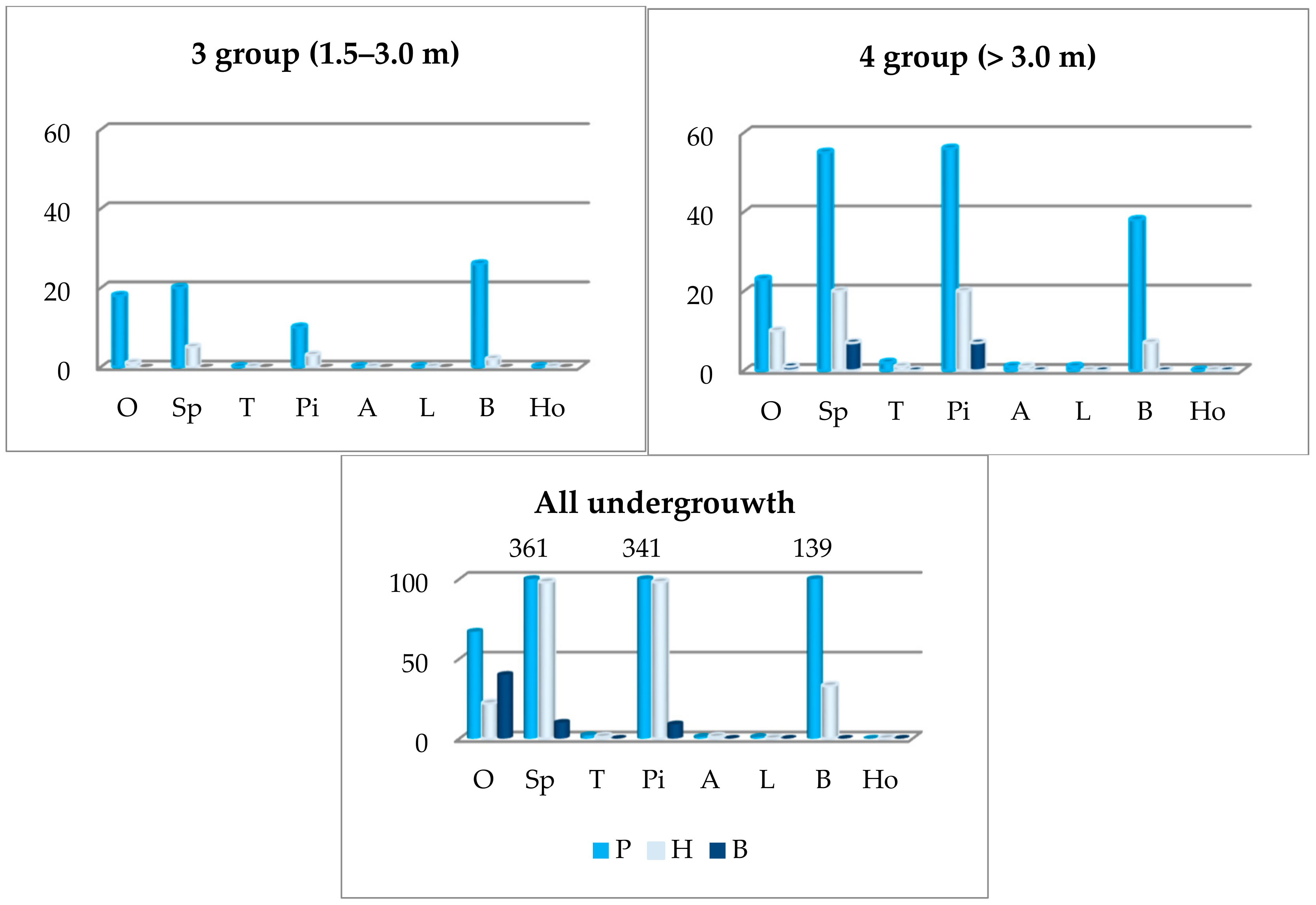
The abundance of oak undergrowth was largest where spruces, pines, and beeches were predominant in the first storey. There was a bit less oak undergrowth in oak sites, and there was very little or none where aspens, alders, limes, and hornbeams were growing in the first storey (Figure 5). The greatest quantity of oak undergrowth in the first group was found where spruces and pines predominated in the first storey. The greatest quantity of the second oak undergrowth group was in the beech and pine sites, the third one in beech and oak sites, and the fourth one in beech and pine sites. The abundance of oak undergrowth is distinguished by individual species of oak. For example, the undergrowth of pedunculated and hybrid oaks was more in the site where beeches, pines and spruces, and sessile oak—where oaks (in the 4 group—pines) dominated in the first storey.
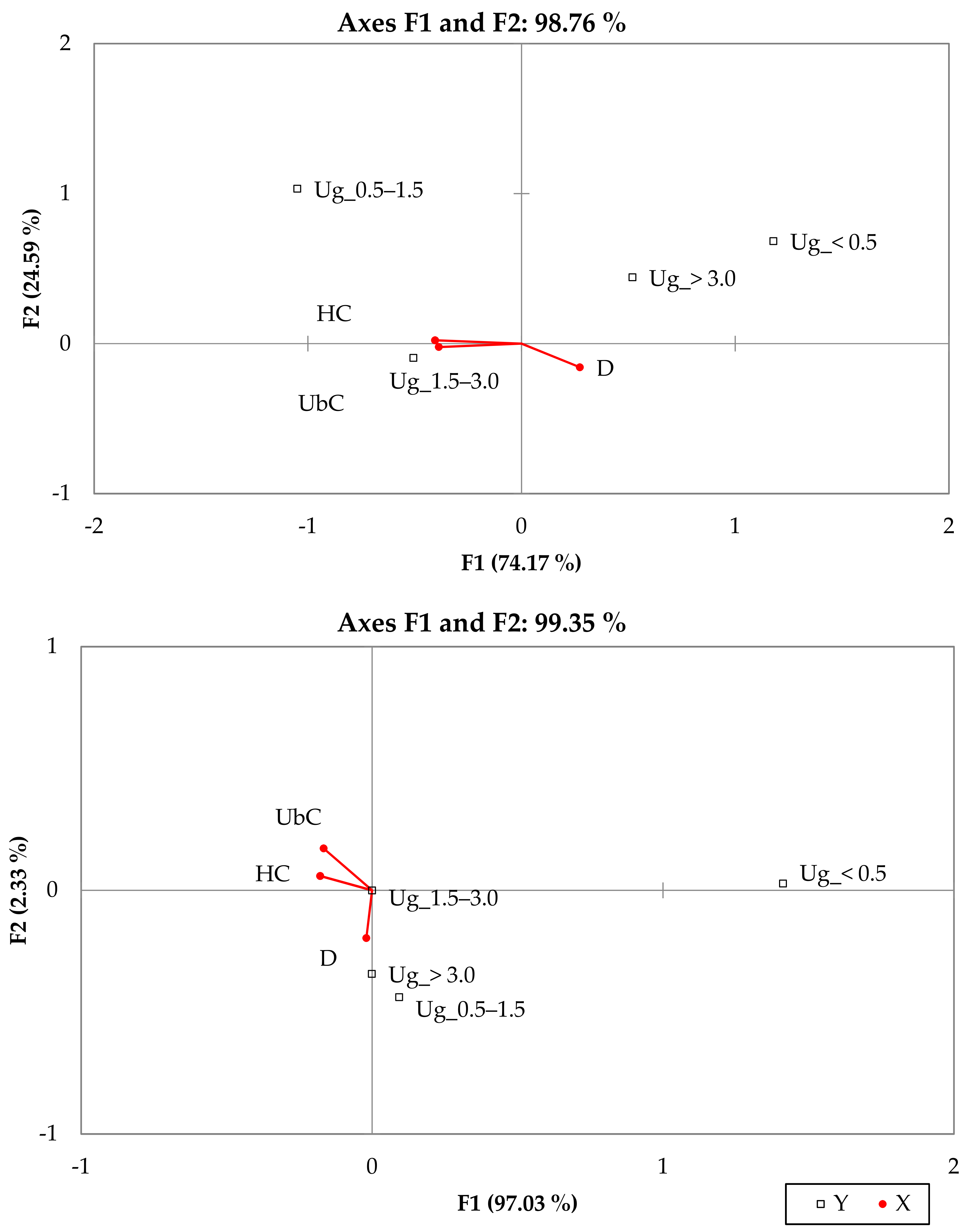
Redundancy analysis (RDA) estimated the coefficients of oak undergrowth abundance depending on density of the first storey, covering of underbrush and herbaceous plants (Figure 6). The RDA showed no linear dependence between x and y variables among all the oak undergrowth, but it was very small linear dependence among hybrid and sessile oaks undergrowth.
Hybrid origin oak undergrowth axis distribution is more similar to that of sessile oak. The density of the first storey had a negative impact for the second undergrowth group’s recovery. Higher underbrush and herbaceous plant covering impact reveal only sessile oak undergrowth. The data showed that fitocenoid structure of the elements influenced oaks of the different height groups unequally. In this case, it would better to analyse by different height groups of undergrowth. Kremer et al. [28] researched results of the process of sessile oak recolonization when one species spreads and becomes established in a certain territory. They found that hybridisation generates other species during generation changes. It is a process that lasts for centuries, in the course of which the oak grows up and starts to prevail in the stands where only a pedunculate oak grew. This leads to increased pollination from pedunculate oak isolation. In summary, the proportion of sessile oaks in the species composition of stands will increase in the future as new sessile oaks are detected in the undergrowth where the first storey of the forest does not contain mature oaks. This conclusion is further confirmed by the spreading of hybrid origin oaks in Trakas Forest, keeping in mind that hybrids are more easily hybridized with sessile oak than with pedunculate oaks.
3.3. Mathematical Modelling of Oak Undergrowth
The number of all founding oaks (Np,g) are summarizes in the mathematical modelling data set. The total results of undergrowth quantity included 4 × 4 size distribution, where interdependence of elements can be evaluated with criterion [30]. Such volume statistics, with 6 degrees of freedom at the 0.05 significance level, were . The quantity of all total undergrowth oak species and age groups was interdependent because statistic is greater than critical. The total undergrowth quantity was an expression of the extensive system properties that can be characteristic only of the study system.
The structural analysis of undergrowth in Trakas Forest showed that a half of all oaks were included in the first height group (up to 0.5 m height). Their quantity was more than 2 times greater than the quantity of the 2nd and 4th height groups of oak (0.5–1.5 m and upper 3 m height). An exception was the 1.5–3 m height group, in which the quantity of oaks did not reach 15% of the quantity of smallest oak height group.
The spreading of undergrowth in the forest characterizes the number of temporary plots where only one oak was found. There were 141 such plots, about 70% of the total number of plots. This suggests that process of oaks' natural regeneration goes evenly. Natural forest covering was even when target tree species account for more than 66% of all plots [31].
The territorial distribution of undergrowth species was rather uneven. The number of plots with sessile oak undergrowth was only 9%. Meanwhile, hybrid oak undergrowth was in 37% of research plots. Statistical analysis showed that the number of plots with oak undergrowth was not interconnected, because statistic was smaller than critical meaning.
The density of undergrowth by systematic point of view was intense, which characterizes its quality. It could not be applied the additivity rule. Therefore, the distribution of undergrowth density was characterized by mean value calculated according to Formula (2). The observed maximum undergrowth density was several times higher than the estimated average of its value (Table 1). They were of the same order of magnitude and fully compatible with undergrowth density values observed by other authors. We determined that in places where oaks regeneration is on-going, the middle number of oaks is 4389 un./ha. This number of undergrowth self-regeneration oak seedlings was closer to the number of oaks in violet-wood sorrel (hepatico-oksalidosa) forest type undergrowth of pure oak forests—5200 un./ha [6]. The average density of the data was more generally characteristic and less dependent on space surveillance and better describes the total Trakas Forest oak undergrowth condition, although it did not reveal the reasons such a condition has occurred. Undergrowth of medium density results, grouped according to their formation time, can be used for different kinds of undergrowth spreading characteristics of the evaluation.
In oak undergrowth formation process, the data, grouped by formation period, revealed that oak undergrowth changes over time. Regrouping the total amount of undergrowth showed a growth compared to the amount of undergrowth in the earliest formative period. Observation time () found the total amount of oak undergrowth from the beginning of its formation had increased about 5 times (Table 2). Growth of sessile and hybrid undergrowth number of oaks decreased more slowly.
In a similar way, the plots of oak undergrowth characterized the spread of forest undergrowth area development (Table 3). The undergrowth area investigated during the life of maximum height oaks expanded about 1.75 times. The data showed that the sessile oak undergrowth spread in the territory progressed by 5% and hybrids even faster, by 11%, than the pedunculate oak. A pedunculate and hybrid oak undergrowth territorially formed in the same places, and their common area increased by only 1.4 times.
The change of quantity of undergrowth and covered territory over time was determined by the investigated undergrowth of four height groups and the qualities described by undergrowth density, calculated according to Formula (7) (Table 4). The calculation shows that Trakas Forest undergrowth’s qualitative characteristics identify the pedunculate oak undergrowth as the dominant mature tree species in the stand. At the time of the study, there were 1047 trees per hectare. The presence of hybrid oak increases this indicator by 3% and, with the addition of sessile oak, by 6%. The density of hybrid and sessile oaks undergrowth there were about 2.5 times less than pedunculate oak.
A more detailed picture of the evolution of the undergrowth formation can be obtained only by mathematical modelling. The main purpose of such mathematical modelling was to define the main factors that determine this process. Both regression analysis to function f (Ap,t) in Equation (7) and analysed variables chosen should be compatible with the characteristics of the test process, and the validity of the obtained dependencies can be solved only on the basis of Fisher criterion (F) and coefficient of determination (R2) values [30]. Therefore, regression analysis was performed on pedunculate and sessile oak species and their hybrids and on the whole oak undergrowth depending on the period and the formation of all possible interactions between variables (Table 5). In the regression analysis, for the purpose of better images, non-absolute values of the density of the oak densities of Ap presented in Table 5 were used, and their relative values at the time of observation (t = 0) were captured in terms of values.
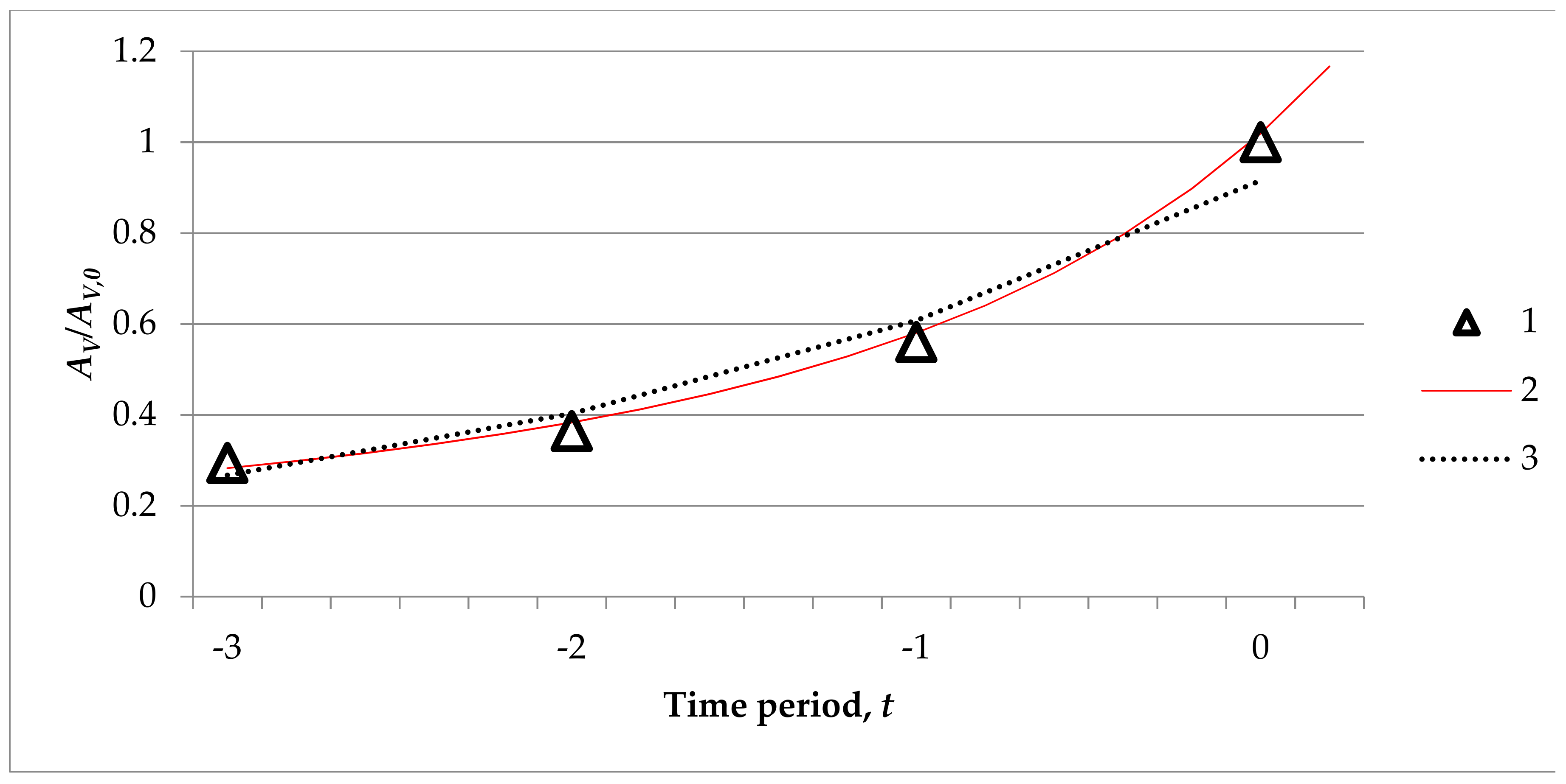
First, let us look at all kinds of oak undergrowth relative density function of time t factor regression analysis of the results presented in Table 5. Total undergrowth evolution can be described not only as the exponential:
but also as the Gompers type of dependence (R2 = 0.996):
The graphic image of such dependence on the time factor (Figure 7, curves 1 and 2) showed a good coincidence with the monitoring data and basically does not have any major advantages than the more complicated Gompers model. Attempts to analyse total oak undergrowth density dependence of two variables basically only confirmed the interdependence (F > Fkr) undergrowth of hybrids (Table 5, line 13). Similar interdependences were determined for undergrowth of pedunculate oak (lines 2 and 3).
For the undergrowth spread, peculiarities analysis was limited to the provided opportunities of monitoring data group exponential regression analysis by depending only on its formation period. Table 5 shows the undergrowth relative density regression analysis, revealing that only pedunculate oak understorey was statistically significant (F > Fkr), although the data determination coefficient was high in all studied oak trees:
The theoretical average undergrowth density dependences (10)–(12) were substantially different only in the exponent indicator in the size parameter m1 by relative approach. The largest average density increase rate was for the undergrowth of pedunculate oak and smallest for sessile oak. The total oak undergrowth density increase rate was higher than the values obtained by individual components (Equation (8)). That strengthening of oak undergrowth density increase rate as one formation property was significant, indicating the effect of the biological system.
The graph image of this research (Figure 7) only additionally confirms the differences of undergrowth average density increase rates of individual undergrowth species and the total oak undergrowth. The higher distribution of oak undergrowth density could be linked with effects of other factors not considered here (cuttings, diseases, etc.). We can neither deny nor confirm that the observations data could be affected by the cuttings in Trakas Forest a decade ago [26]. Despite the fact that undergrowth formation peculiarities were studied only in the formation period, the duration of which was difficult to define, we can conclude that sessile oaks positively influence forest development, because the whole of the undergrowth was formed with higher rates than the individual components of the forest.
The numerical investigation determined that the average density increase of oak undergrowth elements was a significant effect of the system that formed in the course of natural interaction. This oak undergrowth processing feature determines the investigated stand tree species change in the long term.
Other authors’ pedunculate oak undergrowth studies had been limited with extensive features (e.g., the amount of undergrowth and so on), using other monitoring techniques, allowing comparisons to be made only at the level of change trends. In our study, an exponential regression analysis was carried out in Table 4 to present undergrowth’s combined total quantities of all Trakas Forest undergrowth components. The analysis showed that the resulting exponential relative volumes of undergrowth were rather similar (Table 6).
Why the sessile oak exponential rate was much less is related with the already discussed reasons. It can be concluded that in contrast to the average density rate, the relative data of oak undergrowth in respect of formation period varied equally. The pedunculate oak understorey received dependence
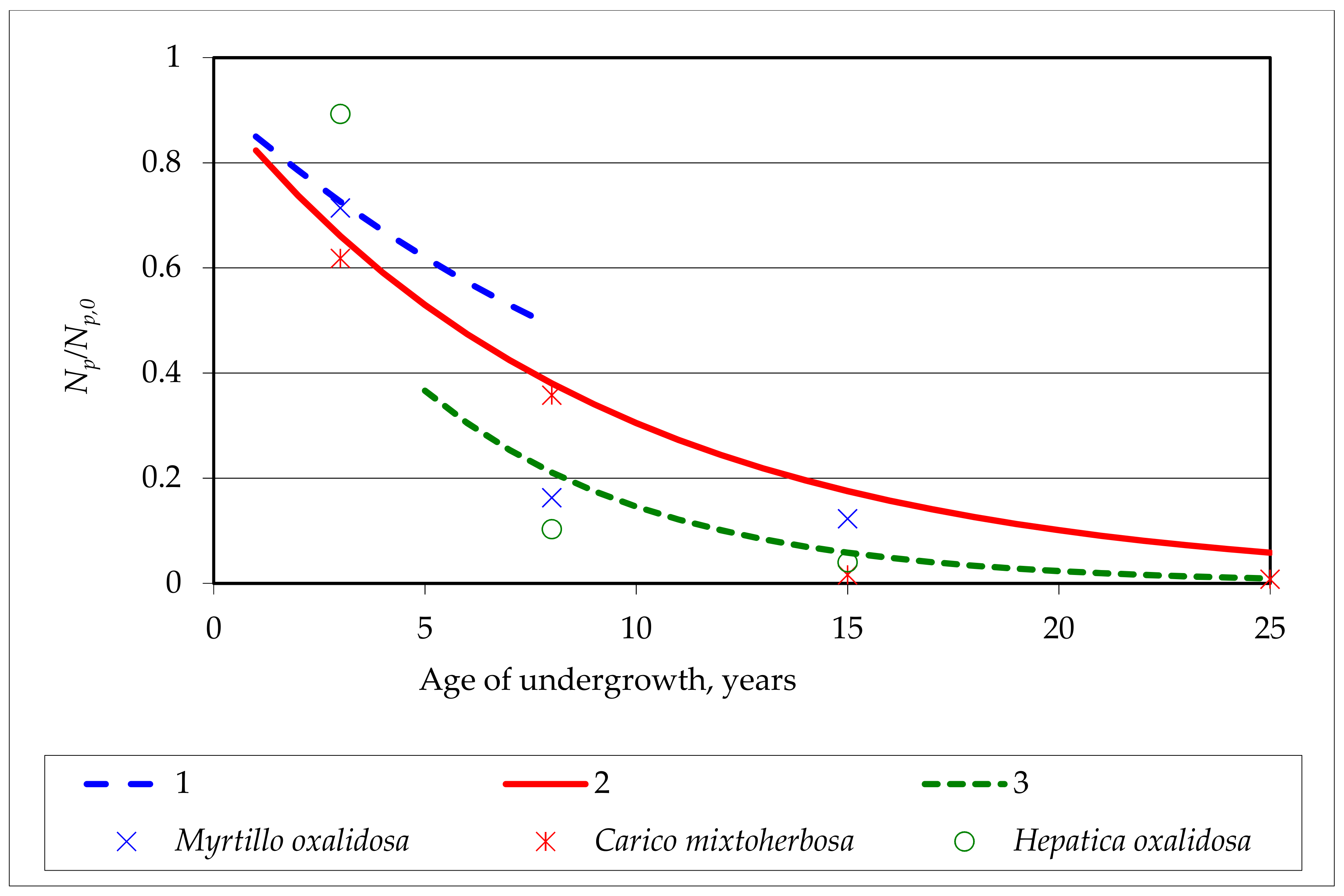
After evaluating the observed age (a) of the oaks, depending on the formation period (t) according to Equation (5), we get the dependence:
The graphic representation of this addition to the condition was fully comparable with the data of other authors [6], which were dependent on the type of oak forest (Figure 8). It might be noted that the formative period of undergrowth could be much shorter than 5 years (Figure 8, curve 1), but from such comparisons, it would be difficult to identify the latest undergrowth period. The age undergrowth was characterized by large variations depending on the type of oak forest, apart from the fact that the observations of other authors did not include all the forest areas. Here the observations on the undergrowth of the relative amount of dependence on the relative amount of undergrowth just shows that this indicator (character) as the extensive feature is more dependent on the species of the whole stand and does not change the relative parameter findings on the undergrowth spread rates. The functional expediency of ongoing processes in undergrowth should be seen in terms in applied forestry, taking into account the characteristics of hybrid oaks, resistance to diseases and pests, and so on.
4. Conclusions
In the mixed Trakas Forest, pedunculate oak predominates. The hybrid oaks are a few times more than sessile oaks. There is determined an increase of hybrid oaks in the undergrowth. The distribution of all oaks is fairly even (70%). But the separate species and their hybrid do not grow evenly. There are more pedunculate and hybrid oaks in the undergrowth where spruces, pines and birches dominate in the first storey and more sessile oaks where oaks, spruces and pines dominate. The undergrowth of oaks is practically non-existent in the aspen, hornbeam and lime sites. The undergrowth of pedunculate oak is mostly distributed in mesoeutrophic and eutrophic soils of normal moisture, and undergrowth of sessile oak in mesoeutrophic soils of normal moisture on slopes and in mesoeutrophic soils of normal moisture. Higher underbrush and herbaceous plant covering impact only sessile oak undergrowth.
Summarizing the mathematical analysis, it can be said that interspecific hybrids in Trakas Forest spread faster than sessile oaks (m1(P) = 0,377, m1(H) = 0.285, m1(S) = 0.238, m1(V) = 0.402), which will in the future change the species composition of stands. Sessile oaks positively influence the development of undergrowth, because a whole undergrowth has formed at a higher rate than the individual components of the undergrowth. Quantitative percentage distribution indicators of oak undergrowth by age groups have similar trends to those obtained by other authors, exploring common oak undergrowth structure of different types of oak and showing that the 5-year period investigating the formation of groups is the right height. We found an increased number of hybrid oaks in the undergrowth. The admixture of sessile oaks in the oak stand had a positive impact on the development of undergrowth.
Author Contributions
Data were collected and analyzed by G.J. and V.B. and G.J. wrote the manuscript.
Acknowledgments
The paper presents research findings that have been obtained through the long-term research programme ‘Sustainable Forestry and Global Changes’ implemented by the Lithuanian Research Centre for Agriculture and Forestry. We thank Habil and Matas Tamonis for consultations in mathematical analysis. Manuscript edited by Cambridge Proofreading and Editing LLC.
Conflicts of Interest
The authors declare no conflict of interest.
References
- Götmark, F.; Kiffer, C. Regeneration of oaks (Quercus robur/Q. petraea) and three other tree species during long-term succession after catastrophic disturbance (windthrow). Plant Ecol. 2014, 215, 1067–1080. [Google Scholar] [CrossRef]
- Navarro, L.M.; Pereira, H.M. Rewilding abandoned landscapes in Europe. In Rewilding European Landscapes; Pereira, H., Navarro, L., Eds.; Springer: New York, NY, USA, 2015; pp. 3–23. [Google Scholar]
- Arroyo-Rodríguezm, V.; Melo, F.P.; Martínez-Ramos, M.; Bongers, F.; Chazdon, R.L.; Meave, J.A.; Tabarelli, M. Multiple successional pathways in human-modified tropical landscapes: New insights from forest succession, forest fragmentation and landscape ecology research. Biol. Rev. 2017, 92, 326–340. [Google Scholar] [CrossRef] [PubMed]
- Vizoso-Arribe, O.; Díaz-Maroto, I.; Vila-Lameiro, P.; Díaz-Maroto, M. Influence of the canopy in the natural regeneration of Quercus robur in NW Spain. Biologia 2014, 69, 1678–1684. [Google Scholar] [CrossRef]
- Goebel, P.C.; Hix, D.M. Development of mixed-oak forests in southeastern Ohio: A comparison of second-growth and old-growth forests. For. Ecol. Manag. 1996, 84, 1–21. [Google Scholar] [CrossRef]
- Karazija, S.; Jurelionis, J.; Vaičiūnas, V. Lietuvos ąžuolynai: Išsaugojimo ir atkūrimo problemos [Lithuanian oak forests: Problems of preservation and restoration]. In Savaiminis ąžuolynų atžėlimas [Self-Contained Regeneration of Oak Trees]; Karazija, S., Ed.; Lututė: Kaunas, Lithuania, 1997; pp. 135–141, (Lithuanian with English summary). [Google Scholar]
- Kullberg, Y.; Bergström, R. Winter browsing by large herbivores on planted deciduous seedlings in southern Sweden. Sweden Scand. J. For. Res. 2001, 16, 371–378. [Google Scholar] [CrossRef]
- Helay, W. Influence of deer on the structure and composition of oak forests in central Massachusetts. In The Science of Overabundance; Mc Shea, W.J., Underwood, H.B., Rappole, J.H., Eds.; Smithsonian Institution Press: Washington, DC, USA, 1997; pp. 249–265. [Google Scholar]
- Lorimer, C.G.; Chapman, J.W.; Lambert, W.D. Tall understory vegetation as a factor in the poor development of oak seedlings beneath mature stands. J. Ecol. 1994, 82, 227–237. [Google Scholar] [CrossRef]
- Brudvig, L.A.; Asbjornsen, H. Dynamics and determinants of Quercus alba seedling success following savanna encroachment and restoration. For. Ecol. Manag. 2009, 257, 876–884. [Google Scholar] [CrossRef]
- Götmark, F. Careful partial harvesting in conservation stands and retention of large oaks favour oak regeneration. Biol. Conserv. 2007, 140, 349–358. [Google Scholar] [CrossRef]
- Kleinschmit, J. Intraspecific variation of growth and adaptive traits in European oak species. Ann. Sci. For. Suppl. 1993, 50, 166–185. [Google Scholar] [CrossRef]
- Bacilieri, R.; Ducousso, A.; Kremer, A. Genetic, morphological and phenological differentiation between Quercus petraea (Matt.) Liebl. and Quercus robur L. in a mixed stand of northwest of France. Silvae Gen. 1995, 44, 1–10. [Google Scholar]
- Jensen, J.S. Provenance variation in phenotypic traits in Quercus robur and Quercus petraea in Danish provenance trials. Scand. J. For. Res. 2008, 23, 179–188. [Google Scholar] [CrossRef]
- Curtu, A.L.; Gailing, O.; Leinemann, L.; Finkeldey, R. Genetic variation and differentiation within a natural community of five oak species (Quercus ssp.). Plant Biol. 2007, 9, 116–126. [Google Scholar] [CrossRef] [PubMed]
- Jensen, J.S.; Hansen, J.K. Geographical variation in phenology of Quercus petraea (Matt.) Liebl. and Quercus robur L. oak grown in a greenhouse. Scand. J. For. Res. 2008, 23, 179–188. [Google Scholar] [CrossRef]
- Abadie, P.; Roussel, G.; Dencusse, B.; Bonnet, C.; Bertocchi, E.; Louvet, J.M.; Kremer, A.; Garnier-Géré, P. Strength, diversity and plasticity of postmating reproductive barriers between two hybridizing oak species (Quercus robur L. and Quercus petraea (Matt) Liebl.). J. Evol. Biol. 2012, 25, 157–173. [Google Scholar] [CrossRef] [PubMed]
- Eriksson, G. Quercus petraea and Quercus robur: Recent Genetic Research; The Silva Slovenica Publishing Centre, Slovenian Forestry Institute: Ljubljana, Slovenia, 2015; p. 104. ISBN 978-961-6993-01-2. [Google Scholar]
- Rupšys, S. Matematinis modeliavimas (miškotvarkoje ir ekologijoje) [Mathematical Modeling (in Forest Management and Ecology)]; LŽŪU LC: Akademija, Lithuania, 2007. [Google Scholar]
- Tuminauskas, S. Bekotis ąžuolas pietų Lietuvoje [Sessile oak in Lithuania]. Mūsų Girios 1957, 5, 11–13. (In Lithuanian) [Google Scholar]
- Patalauskaitė, D. On the quercetalia robori-petraeae in Lithuania. Botanica Lithuanica 2008, 14, 113–119. [Google Scholar]
- Vaičys, M. Miško augaviečių tipai [Types of Forest Sites]; Vaičys, M., Ed.; Lututė: Kaunas, Lithuania, 2006; ISBN 9955-692-41-3. [Google Scholar]
- [WRB] World Reference Base for Soil Resources 2014. International Soil Classification System for Naming Soils and Creating Legends for Soil Maps; World Soil Resources Reports, FAO: Rome, Italy, 2014. [Google Scholar]
- Patalauskaitė, D. Communities of Quercus petraea in Lithuania. Acta Biol. Univ. Daugavp. 2007, 7, 159–164. [Google Scholar]
- Navasaitis, M.; Ozolinčius, R.; Smaliukas, D.; Balevičienė, J. Lietuvos dendroflora [Dendroflora in Lithuania]; Lututė: Kaunas, Lithuania, 2003. (In Lithuanian) [Google Scholar]
- Baliuckas, V. Paprastojo (Quercus robur) ir bekočio ąžuolo (Q. petraea) rūšių introgresija Trako miške (Introgression of pedunculate (Quercus robur) and sessile (Q. petraea) oak species in Trakas Forest). Bot. Lith. 2000, 6, 375–387. [Google Scholar]
- Carlise, A.; Brown, A.F. The assessment of the taxonomic status of mixed oaks (Quercus ssp.) populations. Watsonia 1965, 6, 120–127. [Google Scholar]
- Kremer, A.; Dupouey, J.L.; Deans, J.D.; Cotrell, J.; Csaikl, U.; Finkeldey, R.; Espinel, S.; Jensen, J.; Kleinschmit, J.; Van Dam, B.; et al. Leaf morphological differentiation between Quercus robur and Quercus petraea is stable across western European mixed oak stands. Ann. For. Sci. 2002, 59, 777–787. [Google Scholar] [CrossRef]
- Borazan, A.; Babaç, M.T. Morphometric leaf variation in oaks (Quercus) of Bolu Turkey. Ann. Bot. Fenn. 2003, 40, 233–242. [Google Scholar]
- Čekanavičius, V.; Murauskas, G. Statistika ir jos taikymai [Statistics and Its Applications]; TEV: Vilnius, Lithuania, 2001. (In Lithuanian) [Google Scholar]
- [LR AM] LR AM Miškų departamentas. Miško atkūrimas ir veisimas (Teisės aktų rinkinys) [Reforestation and Breeding (Legislative Package)]; UAB Lodvila: Vilnius, Lithuania, 2011. (In Lithuanian) [Google Scholar]
Figure 1.
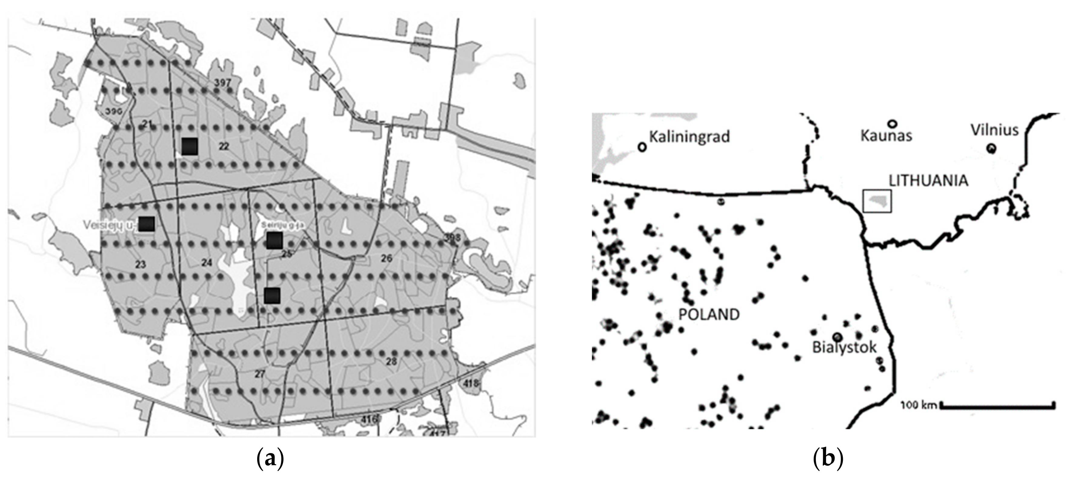
Trakas Forest in Alytus district, Veisiejai Forest Enterprise, Seirijai Forest District in Lithuania (54°14′11″ N, 23°45′30″ E, 190 m a.s.l.): (a) circles—locations of the sampling sites of the undergrowth; squares—the location of sampling sites of the first storey of the stand in Trakas Forest; numbers and lines indicate forest blocks; (b) rectangular area shows the location of Trakas Forest in Lithuania and smaller black circles indicate the nearest natural sessile oak stands in Poland.
Figure 1.
Trakas Forest in Alytus district, Veisiejai Forest Enterprise, Seirijai Forest District in Lithuania (54°14′11″ N, 23°45′30″ E, 190 m a.s.l.): (a) circles—locations of the sampling sites of the undergrowth; squares—the location of sampling sites of the first storey of the stand in Trakas Forest; numbers and lines indicate forest blocks; (b) rectangular area shows the location of Trakas Forest in Lithuania and smaller black circles indicate the nearest natural sessile oak stands in Poland.

Figure 2.
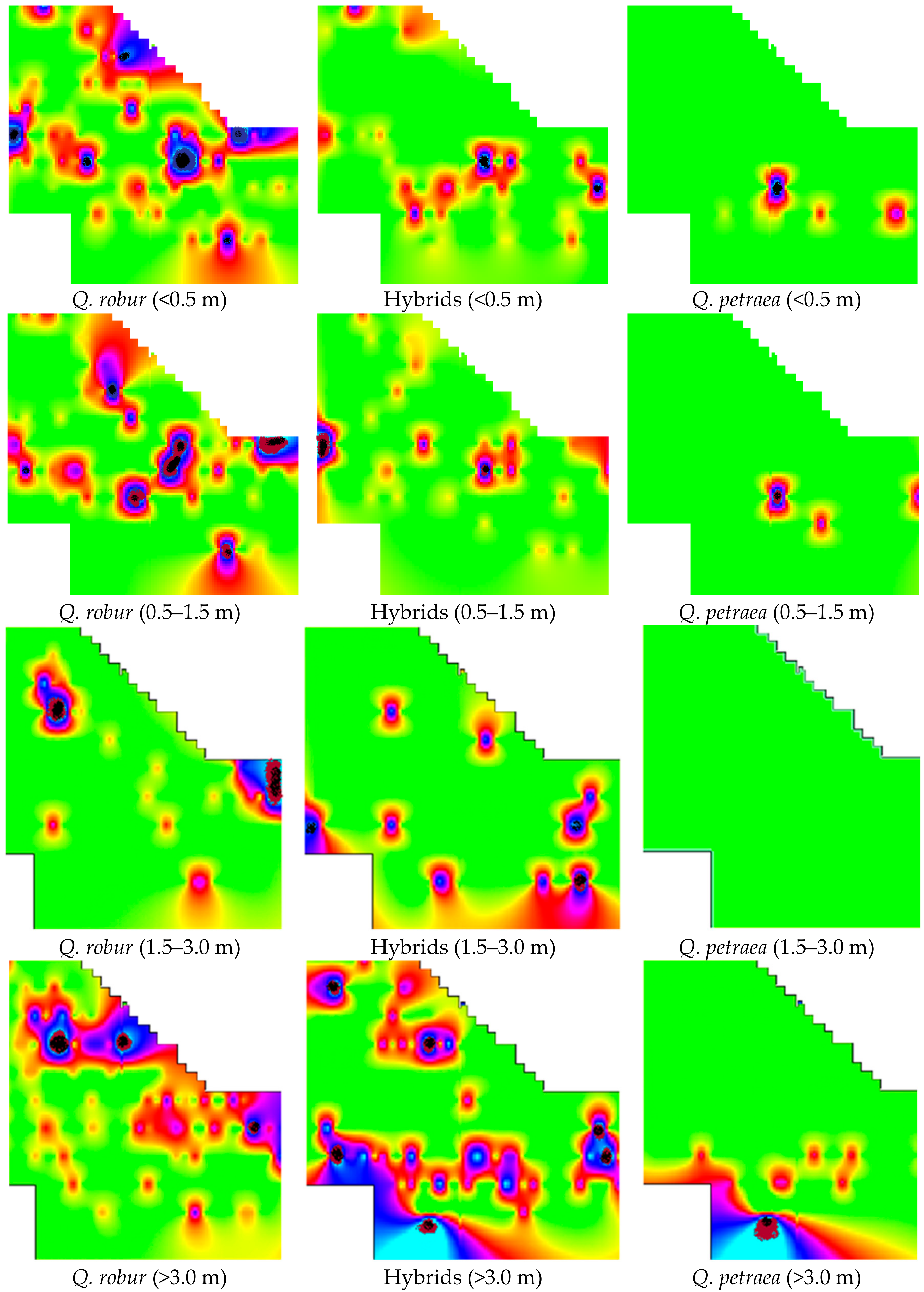
Oak undergrowth distribution by height groups and species. Brightest colour indicates an area where there is no oak undergrowth. Different colours indicate differing numbers of oaks in the plots. The plot area is 78.5 m2. The largest number of oak undergrowth in the group up to 0.5 m height was: for Q. robur, 26; hybrids, 15; Q. petraea, 17. Respectively, in the group with height 0.5–1.5 m: 13, 13, 3; in the group of 1.5–3.0 m height: 10, 2, 0; and in the group with height over 3.0 m: 10, 3, 4.
Figure 2.
Oak undergrowth distribution by height groups and species. Brightest colour indicates an area where there is no oak undergrowth. Different colours indicate differing numbers of oaks in the plots. The plot area is 78.5 m2. The largest number of oak undergrowth in the group up to 0.5 m height was: for Q. robur, 26; hybrids, 15; Q. petraea, 17. Respectively, in the group with height 0.5–1.5 m: 13, 13, 3; in the group of 1.5–3.0 m height: 10, 2, 0; and in the group with height over 3.0 m: 10, 3, 4.

Figure 3.
The first stand storey (larger circles) and undergrowth (smaller circles) distribution by species in four study plots of 0.5 ha each. The letters of legend indicate: P—pedunculate oak, H—hybrid oak, S—sessile oak.
Figure 3.
The first stand storey (larger circles) and undergrowth (smaller circles) distribution by species in four study plots of 0.5 ha each. The letters of legend indicate: P—pedunculate oak, H—hybrid oak, S—sessile oak.

Figure 4.
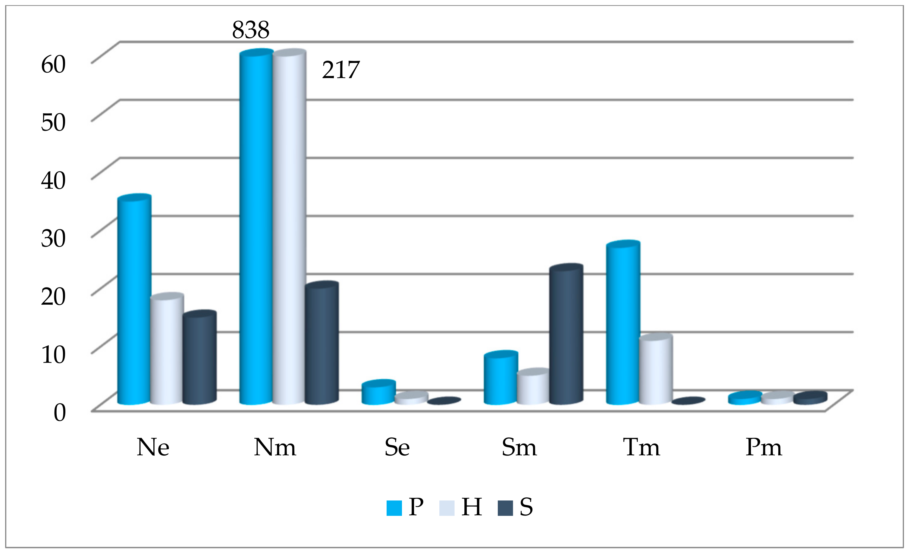
Abundance of oak undergrowth (P—pedunculate oak, H—hybrid oak, S—sessile oak) in different forest sites: Ne—eutrophic soils of normal moisture, Nm—mesoeutrophic soils of normal moisture, Se—eutrophic soils of normal moisture on slopes (>15°), Sm—mesoeutrophic soils of normal moisture on slopes (>15°), Tm—mesoeutrophic gleyic soils of temporary overmoisture, Pm—mesoeutrophic gley soils of permanent overmoisture.
Figure 4.
Abundance of oak undergrowth (P—pedunculate oak, H—hybrid oak, S—sessile oak) in different forest sites: Ne—eutrophic soils of normal moisture, Nm—mesoeutrophic soils of normal moisture, Se—eutrophic soils of normal moisture on slopes (>15°), Sm—mesoeutrophic soils of normal moisture on slopes (>15°), Tm—mesoeutrophic gleyic soils of temporary overmoisture, Pm—mesoeutrophic gley soils of permanent overmoisture.

Figure 5.
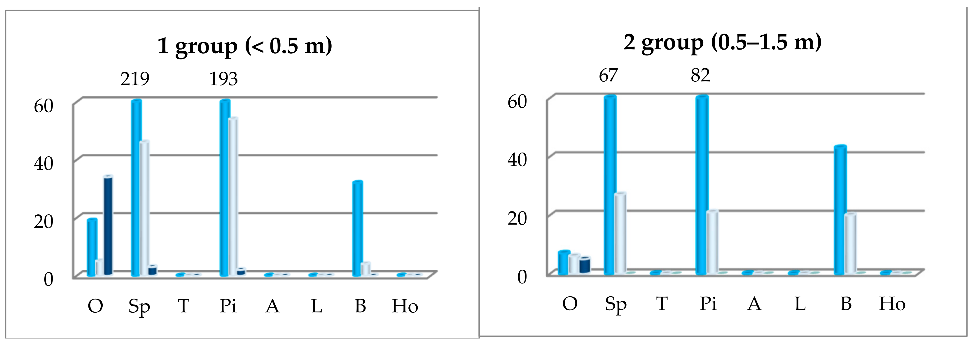
The abundance of oak undergrowth depending on the first storey prevailing species: P—pedunculate oak, H—hybrid oak, S—sessile oak. In the x array: O—oak sp., Sp—Norway spruce, T—the total oak undergrowth, Pi—silver pine, A—black alder, L—small-lived lime, B—common birch, Ho—common hornbeam.
Figure 5.
The abundance of oak undergrowth depending on the first storey prevailing species: P—pedunculate oak, H—hybrid oak, S—sessile oak. In the x array: O—oak sp., Sp—Norway spruce, T—the total oak undergrowth, Pi—silver pine, A—black alder, L—small-lived lime, B—common birch, Ho—common hornbeam.


Figure 6.
The vector distribution between two axes (RDA): pedunculate oak (top), sessile oak (lower) and their hybrid (middle) in four undergrowth (Ug) height classes (y) and their dependence from site density (D) and covering of underbrush (UbC) and herbaceous plant (HC) (x).
Figure 6.
The vector distribution between two axes (RDA): pedunculate oak (top), sessile oak (lower) and their hybrid (middle) in four undergrowth (Ug) height classes (y) and their dependence from site density (D) and covering of underbrush (UbC) and herbaceous plant (HC) (x).


Figure 7.
The dependence of the relative density (AV/AV,0) on the total oak undergrowth in the formation period: 1—data of observations, 2—Gomperz curve, 3—exponent curve.
Figure 7.
The dependence of the relative density (AV/AV,0) on the total oak undergrowth in the formation period: 1—data of observations, 2—Gomperz curve, 3—exponent curve.

Figure 8.
Relative amount of exponential dependence on the age of the pedunculate oak undergrowth compared with other authors’ observation data in different oak stands: 1—exponential curve to Δt = 3 year, 2—exponential curve to Δt = 5 year, 3—an exponential curve to Δt = 7 years. Points—data of observations [6].


Table 1.
The average density of oak undergrowth (Ap,g), units/ha (Equation (2)).
| Oaks (p) | Undergrowth Height Group (g) | Average Density (Ap) | The Maximum Density ( | |||
|---|---|---|---|---|---|---|
| 1 | 2 | 3 | 4 | |||
| Sessile oak | 621 | 212 | 0 | 191 | 418 | 2930 |
| Hybrid 1 oak | 479 | 363 | 140 | 193 | 436 | 3822 |
| Pedunculate oak | 867 | 539 | 449 | 335 | 1047 | 4586 |
| Total species | 895 | 621 | 401 | 328 | 1106 | 8408 |
1 In all the tables, data shown of first and other generations interspecific hybrids between pedunculate and sessile oaks.
Table 2.
The total amount (Np,t) of oak trees in the undergrowth in plots dependent on the formation period (t) in years (Equation (3)).
Table 2.
The total amount (Np,t) of oak trees in the undergrowth in plots dependent on the formation period (t) in years (Equation (3)).
| Oaks (p) | Period of Undergrowth Formation | Relative Amount of Undergrowth | ||||
|---|---|---|---|---|---|---|
| t = −3 | t = −2 | t = −1 | t = 0 | Np,0/Np,−3 | % | |
| Sessile oak | 15 | 15 | 20 | 59 | 3.9 | 0.048 |
| Hybrid oak | 59 | 70 | 144 | 253 | 4.3 | 0.21 |
| Pedunculate oak | 176 | 250 | 449 | 912 | 52 | 0.74 |
| Total undergrowth | 250 | 335 | 613 | 1224 | 4.9 | 100 |
Table 3.
Dependence of occupied number of plots (Bp,t) of oak trees in the undergrowth by the formation period (t) in years (Equation (5)).
Table 3.
Dependence of occupied number of plots (Bp,t) of oak trees in the undergrowth by the formation period (t) in years (Equation (5)).
| Oaks (p) | Period of Undergrowth Formation (t) | Relative Amount of Plot Numbers Bp,0/Bp,−3 | |||
|---|---|---|---|---|---|
| t = −3 | t = −2 | t = −1 | t = 0 | ||
| Sessile oak | 10 | 10 | 13 | 18 | 1.8 |
| Hybrid oak | 39 | 49 | 67 | 74 | 1.9 |
| Pedunculate oak | 67 | 73 | 92 | 111 | 1.7 |
| Total | 97 | 106 | 125 | 141 | 1.5 |
Table 4.
Oak trees in the undergrowth density change (Ap,t) dependent on the formation period, units/ha (Equation (6)).
Table 4.
Oak trees in the undergrowth density change (Ap,t) dependent on the formation period, units/ha (Equation (6)).
| Oaks (p) | Period of Undergrowth Formation (t) in Years | |||
|---|---|---|---|---|
| t = −3 | t = −2 | t = −1 | t = 0 | |
| Sessile oak | 191 | 191 | 196 | 418 |
| Hybrid oak | 193 | 182 | 274 | 436 |
| Pedunculate oak | 335 | 436 | 622 | 1047 |
| Total | 328 | 403 | 625 | 1106 |
Table 5.
The relative density of the development of oak trees in the undergrowth, with group regression analysis (Equation (7)).
Table 5.
The relative density of the development of oak trees in the undergrowth, with group regression analysis (Equation (7)).
| No. | Function of Undergrowth Status | Critical Value of Criterion F | Indexes | ||||
|---|---|---|---|---|---|---|---|
| Criterion F | Determination Coefficient (R2) | Constant (C) | Coefficient | Coefficient m1 | |||
| Quercus robur | |||||||
| 1 | AP/AP,0= f (t) | 18.5 | 84.7 | 0.977 | 0.934 | 0.377 | |
| 2 | AP/AP,0= f (t, AH/AH,0) | 200 | 487 | 0.999 | 0.525 | 0.636 | 0.258 |
| 3 | AP/AP,0= f (t, AS/AS,0) | 200 | 290 | 0.998 | 0.49 | 0.432 | 0.306 |
| Quercus petraea | |||||||
| 5 | AS/AS,0= f (t) | 18.5 | 3.4 | 0.626 | 0.799 | 0.238 | |
| 6 | AS/AS,0= f (t, AH/AH,0) | 200 | 5.8 | 0.920 | 0.153 | 1.828 | −0.107 |
| 7 | AS/AS,0= f (t, AP/AP,0) | 200 | 38.9 | 0.988 | 0.077 | 2.549 | −0.328 |
| Hybrid oak | |||||||
| 8 | AH/AH,0= f (t) | 18.5 | 10.6 | 0.841 | 0.896 | 0.285 | |
| 9 | AH/AH,0= f (t, AP/AP,0) | 200 | 11 | 0.957 | 0.228 | 1.500 | −0.046 |
| 10 | AH/AH,0= f (t, AS/AS,0) | 200 | 6.4 | 0.927 | 0.494 | 0.708 | 0.169 |
| Total | |||||||
| 11 | AV/AV,0= f (t) | 18.5 | 49.3 | 0.961 | 0.917 | 0.409 | |
| 12 | AV/AV,0= f (t, AP/AP,0) | 200 | 120 | 0.996 | 0.336 | 1.098 | 0.165 |
| 13 | AV/AV,0= f (t, AH/AH,0) | 200 | 8891 | 0.999 | 0.398 | 0.922 | 0.235 |
| 14 | AV/AV,0= f (t, AS/AS,0) | 200 | 50.3 | 0.990 | 0.577 | 2.549 | −0.328 |
Table 6.
Group regression analysis of the dependence of the formation period of the total amount (Np,t) of oak trees undergrowth.
Table 6.
Group regression analysis of the dependence of the formation period of the total amount (Np,t) of oak trees undergrowth.
| Function of Undergrowth Condition | Critical Value of Criterion F | Indexes | |||
|---|---|---|---|---|---|
| Oaks | Criterion F | Determination Coefficient (R2) | Constant (C) | Coefficient (m1) | |
| Sessile oak | 18.5 | 94 | 0.979 | 0.920 | 0.552 |
| Hybrid oak | 18.5 | 41 | 0.953 | 0.939 | 0.509 |
| Pedunculate oak | 18.5 | 6 | 0.760 | 0.744 | 0.440 |
| Total | 18.5 | 68 | 0.972 | 0.915 | 0.537 |
© 2018 by the authors. Licensee MDPI, Basel, Switzerland. This article is an open access article distributed under the terms and conditions of the Creative Commons Attribution (CC BY) license (http://creativecommons.org/licenses/by/4.0/).
Share and Cite
MDPI and ACS Style
Jurkšienė, G.; Baliuckas, V. Pedunculate and Sessile Mixed Oak Forest Regeneration Process in Lithuania. Forests 2018, 9, 459. https://doi.org/10.3390/f9080459
AMA Style
Jurkšienė G, Baliuckas V. Pedunculate and Sessile Mixed Oak Forest Regeneration Process in Lithuania. Forests. 2018; 9(8):459. https://doi.org/10.3390/f9080459
Chicago/Turabian StyleJurkšienė, Girmantė, and Virgilijus Baliuckas. 2018. "Pedunculate and Sessile Mixed Oak Forest Regeneration Process in Lithuania" Forests 9, no. 8: 459. https://doi.org/10.3390/f9080459
Note that from the first issue of 2016, this journal uses article numbers instead of page numbers. See further details here.