Modeling Lean and Agile Approaches: A Western Canadian Forest Company Case Study

Abstract

In the forest supply chain of the coast of British Columbia, the material flows are directed toward the push production of commodity products. This industry has not adopted lean and agile principles due to unclear economic impacts on the supply chain in changing market conditions. We tested the ability of lean and agile principles to improve performance in the coastal integrated forest industry. Mixed integer programming formulations were subject to over–under production capacity, and over–under demand fulfillment penalties to emulate agile, lean, and hybrid manufacturing environments, when solving the planning problem. Assuming that the coastal integrated forest industry performs as a hybrid environment, the profit results of each manufacturing environment were judged. The results show that, opportunities for profit improvement were 11% for adopting an agile environment when demand was stable with low variation and large batches of production. However, profit improvement was non-existent when the same demand attributes apply but with high variation. The opportunities for profit improvement were 12% when an agile environment or lean environment was adopted when demand was stable with low variation and small batches of production. However, opportunities for profit improvements of 15% existed for adopting an agile environment when demand was unstable with high variation and small batches of production.

1. Introduction

A large number of companies are thinking to switch to lean and agile manufacturing systems [1]. Supply chain managers strongly rely on their ability to reduce costs and waste, increase customer service, and provide a competitive advantage. Lean and agile manufacturing systems are multi-dimensional approaches that contain a variety of management practices. Resources efficiency and high performance are key stones of lean manufacturing, while the capabilities of addressing customer requirements are on the side of agile manufacturing [2].

Lean manufacturing can be described as developing a value stream to eliminate all waste including time, and ensure a level schedule [3]. A manufacturing process working away from variation and uncertainty can be defined as a level schedule, which ensures high capacity utilization, thus leading to lower manufacturing costs. Consequently, lean manufacturing is a system mainly that is focused on increasing the efficiency of operations. Contrarily, [4] agile manufacturing is a system that is capable of operating profitably in a competitive environment, where customer demands continuously and unpredictably change. Agility reacts quickly and effectively to changing customer needs in a volatile marketplace; it is able to handle variety and introduce new products. The ability to introduce highly customized products is a key component of agile systems, which is addressed with capabilities to change between products without significant investment. However, such flexibility increases manufacturing and transportation costs [5]. Thus, a lean manufacturing approach is predominant in production systems that are focused on products that satisfy basic needs, where the products demand is stable with large life cycles. Contrarily, an agile manufacturing approach is predominant in production systems that advocate innovative products that satisfy sophisticated needs, where the products demand is almost unpredictable with short life cycles [6].

The adoption of emergent manufacturing systems principles should be subject to accurate economic analyses. However, there is no substantive economic evidence at the bottom of the economic forest company level to support their implementation. Hence, we reviewed the related literature to suggest a framework to address manufacturing system evaluation.

This type of systems evaluations have been performed using discrete event simulation (DES) models, measuring their advantages in different industries when adopting lean, agile, and hybrid principles, but only at the shop floor level of the factory [1]. On the other hand, mixed-integer linear programming (MIP) models have been used to elucidate the ability of agile principles in order to improve the economic performance for supply chain network design. Strategic and tactical decisions such as opening facilities and their capacities, and selecting transportation modes were considered [7]. Although the previous research is novel, it does not address the short-term aggregate planning problem where the ability of the manufacturing system must be measured.

Lean, agile, and hybrid manufacturing are philosophies that are easy to understand; however, their complexity appears during implementation. Goldsby et al. [1] modeled a supply chain (SC) for lean, agile, and hybrid manufacturing to evaluate their benefits and tradeoffs. A DES model was used to simulate the SC. The results showed costs, lead times, and inventory tradeoff between manufacturing environments. However, there was no mention of how product demand patterns should be assessed in order to better represent the manufacturing philosophies. Another attempt to quantify lean manufacturing benefits was made by Al-Aomar et al. [8]. The manufacturing system was modeled with DES, and a tabu search approach (TS) was used to find the model parameters that optimized the lean measures (e.g., work in process (WIP) and lead times (LT)). As lean measures with one objective could be contradictory, a multi-objective cost function to rank solutions at each TS step was applied. Although this approach considered the effect of lean techniques on profits, it is not clear how this method balanced lean measures, as the author claimed.

Despite efforts to measure the benefits of manufacturing systems with models, most research has been conducted for only one facility, regardless of the effect on the SC, and without considering demand changes [9]. Until now, researchers have been applying DES, value stream mapping (VSM), experimental design, and TS to find the setting that optimizes the balance between manufacturing measures. These approaches have been successful when modeling floor variables, given their stochastic nature. Unfortunately, these efforts fail to explicitly measure the impact of the manufacturing principles on economic performance. On the other hand, MIP have been used to optimize short-term production planning [10], where policies to manage inventory, production capacity, customer service, and lead times can be easily tested. Thus, the mid and short-term production planning problem represents a suitable scenario for testing lean, agile, and hybrid manufacturing environments.

The SC uses raw materials, which are resources with limited capacities to produce products that satisfy customer demand, optimizing the tradeoff between setup and inventory holding costs [11]. The problem has been solved with MIP formulations. Furthermore, Billington et al. [12] suggest that the problem begins when material requirement planning (MRP) systems assume no constraints for facilities; hence, any amount of production is presumed to be possible in each facility. However, lead times (setup and production time) can increase due to bottleneck operations, triggering unpredictable lead times. This problem has been called a capacity-constrained production scheduling problem.

Depending on the manufacturing system, different modeling approaches can be applied. A tradeoff analysis between setup and holding inventory costs should be conducted [10]. Multiple products and capacity constraints increase the complexity of the problem. The MIP formulations usually focus on minimizing the setup and holding inventory costs, which are subject to material balance constraints, plus capacity and market constraints. However, in practice, the number of binary and continuous variables (i.e., production quantities by product and setup cost) makes the problem intractable with exact algorithms.

MRP calculates the requirements for all items, including raw materials, parts, components, and subassemblies. MRP determination is based on master planning scheduling, capacity requirement planning, and lot-sizing determinations. Lot-sizing decisions may be made based on previous requirements, and always consider materials, machines, and labor constraints. If there are capacity constraints, this problem could become a single or multiple-level capacitated lot-sizing problem [13].

In this context, the well-defined and rich literature on lean tools and methods is contradicted by a few documented quantitative implementations [14] in which the value of lean manufacturing using DES and VSM was tested. A pull strategy to reduce WIP and LT in relation to a push strategy (i.e., large WIP and LT) was assessed, but there are no details on how the pull future state was developed.

Although there is evidence that lean manufacturing techniques (i.e., Just In Time (JIT), total preventive maintenance (TPM), and cellular manufacturing) improve performance in discrete manufacturing, evidence on continuous production is scarce. Aldulmalek et al. [15] performed an analysis of a continuous manufacturing process based on DES, VSM, and historical data. They introduced buffers and scheduling around the bottleneck work station. Later, a DES was run and set up with two levels of TPM, two setup times, and push and hybrid pull manufacturing. Their results showed that pull hybrid manufacturing and TPM trigger significant lead-time reductions, as well as strong reductions in WIP.

Consequently, we sorted a hierarchically and translated lean, agile, and hybrid principles into planning drivers. As a matter of fact, the literature on manufacturing systems is extensive, yet few quantitative implementations can be found, and almost no publications are available for forest industry applications. Meanwhile, not all of the drivers that were mentioned in the literature can be translated and used in a mathematical formulation. We summarized the key drivers based on a large but not extensive literature review, as shown in

Table 1. Attributes of lean, agile, and hybrid manufacturing supply chain (SC) drivers.

Driver	Lean	Agile	Hybrid
SC strategy	Costs leadership, zero waste, flexibility and incremental improvements for existing product production.	Differentiation responsiveness, site of inventory capacity: responsiveness. Provides customized products with short lead times by reducing the costs of variety.	Mass customization by postponing product differentiation until final assembly.
Product attributes	Functional commodity: Highly predictable, long life cycles (e.g., a staple).	Innovative: uncertain demand, short life cycles (e.g., a customized laptop).	Mixed portfolio: functional and innovative components. Long–short life cycles (e.g., a car).
Volume-variety	Large volumes of low variety.	Small volumes of high variety.	Both.
Demand	Stable and predictable.	Unstable and unpredictable.	Both.
Manufacturing focus	Maintains high average utilization rate. Level strategy.	Deploys excess buffer capacity to ensure that raw materials are available to manufacture. Chase strategy.	Part chase strategy and part level strategy.
Back orders	Allowed but penalized.	Not allowed or highly penalized.	Both mixed.
Inventory policy	Generates high turnover and minimize inventory.	Deploys significant stocks of parts to tide over unpredictable market needs.	Minimizes functional component inventories.
Lead time focus	Shorten lead times as long as it does not increase cost.	Invests aggressively in ways to reduce lead times.	Lean at component level. However, at the product level, follows agile focus.
Decoupling Point (DP)	At warehouse site	At manufacturing site	At manufacturing site

(detailed information can be found at Hallgren et al. [2,3,6,16,17,18,19,20,21]. Translation of the drivers was applied later on the model formulation of each manufacturing environment (ME).

The current manufacturing system of the British Columbia forest industry lacks a differentiation of manufacturing systems by product demand, assuming that a high rate of utilization and increasing throughput are good enough to keep the competitiveness [22]. This industry does not recognize the ability of an agile system to capture higher value when producing highly customized lumber products. However, due to the changeable lumber market conditions, it is necessary to test emerging manufacturing systems to explore the benefits for this industry.

The objective of this research was to determine the impact on profits due to the decision of changing the manufacturing system. We first translated manufacturing system soft drivers into hard mathematical constraints. Second, we formulated three MIP optimization models that represent lean, agile, and hybrid manufacturing systems to solve the forest-to-lumber planning problem. Third, these models were applied under different lumber demand scenarios to represent the variability faced by the forest industry [1,6]. A Coastal British Columbia integrated forest company was chosen as the case study. The aim of this study was to explore the relationships between lean–agile–hybrid drivers and decision outcomes, highlighting their benefits and tradeoffs. To our knowledge, this is the first initiative in which lean, agile, and hybrid manufacturing systems have been evaluated and compared based on soft drivers translated into hard constraints to be modeled with mathematical programming. This study first provides descriptions of the essential drivers of the manufacturing systems, previous research, and a detailed case study. Then, a methodology to model the manufacturing principles is explained, followed by the results of the assessment of the performance of the manufacturing environment. The final sections contain discussion and conclusions, where highlights and conclusions on selecting manufacturing principles are explained.

2. Materials and Methods

For better understanding, this section was divided into three sections. First is the case study, where we explain its singularities and sources of data. Second, the formulation of models was conceptually addressed, where we translate the manufacturing drivers into mathematical programming models. Third, we explain how the lumber demand scenarios were developed, which helped to recreate lumber demand behaviors based on order sizes and variability inside the order.

2.1. The Case Study

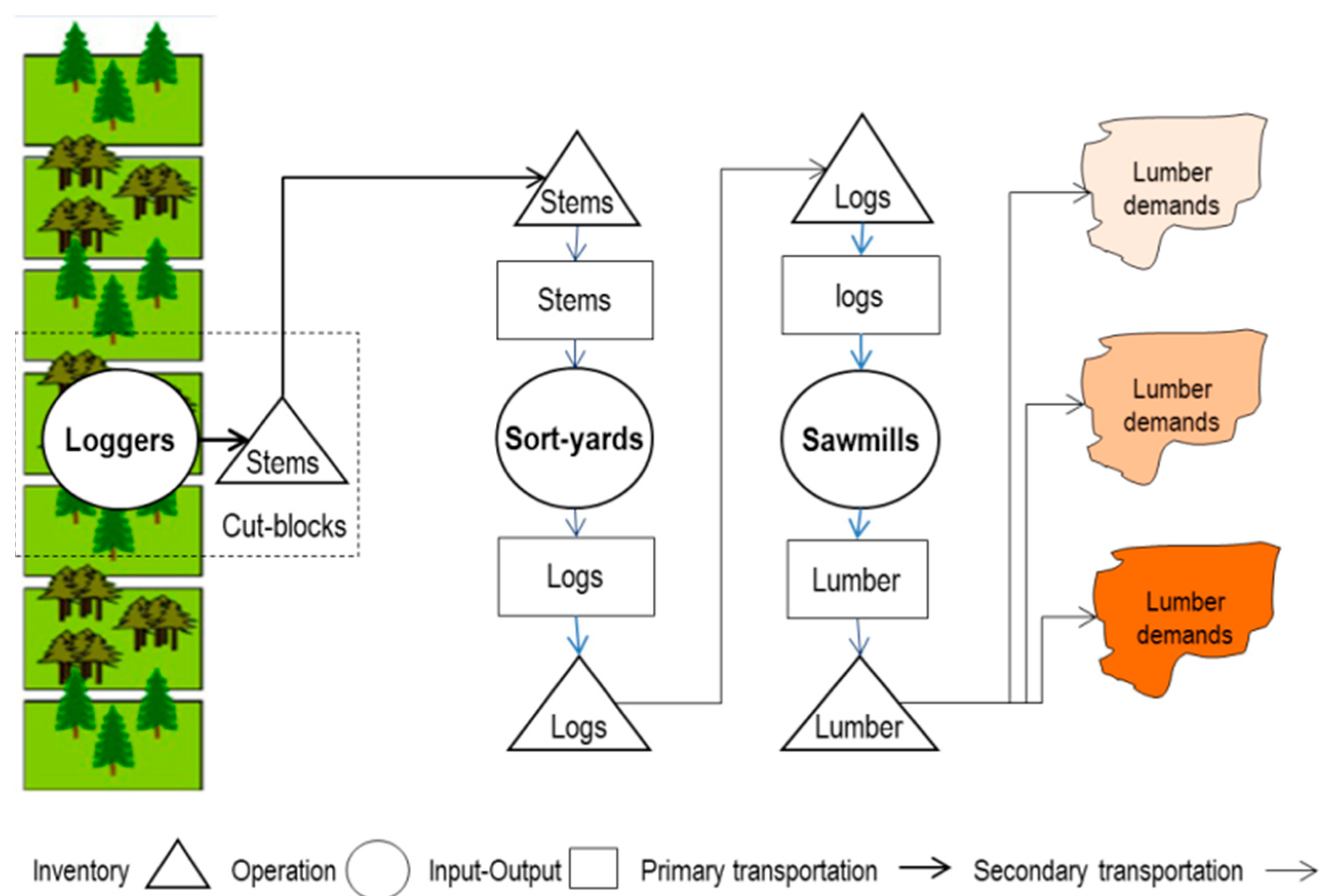
The forest-to-lumber SC planning problem was formulated keeping in mind an integrated BC Coastal forest SC, where harvesting, sort-yarding, and sawmilling operations do not always happen simultaneously [22]. A year-based forest operation begins with logging, and then the logs for sawmilling are sorted by species, grade, and hauled by ground or water directly to forest industries. Downstream, sawmills extract the highest lumber grades possible from logs to produce commodities and customized lumber products [23]. In terms of sales, when construction lumber grades are traded, wholesalers tend to be tolerant of an over/under fulfillment of orders. However, when trading high-grade lumber, industrial and wholesaler customers are less tolerant (i.e., there are high penalizations for missing targets). The focus in coastal BC is to create value while maintaining high volume and value recoveries and capacity utilization. Consequently, for the purpose of this study, a year of operation was considered as the time window. Accordingly, a planning horizon of one year divided into four periods was chosen (four quarters). The problem can be divided into procurement planning and lumber planning, where loggers carry out harvesting plans in advance and push stems and logs to sort yards. Then, sawmills buy log sorts depending on lumber sales orders, which is why the decoupling point of this SC is located at the sort yards (Figure 1).

A case study provides the data for forest inventory yields, harvesting costs, log-to-lumber yields, manufacturing costs, lumber prices, and sales orders, and such information was extracted from publicly available annual financial reports from a British Columbia (BC) coastal forest integrated company [24].

2.2. Formulation of Models

The soft drivers of manufacturing principles were translated into hard drivers to model the problem. The SC strategy driver of the ME was considered as the central driver and used as the objective function. The manufacturing focus and inventory policy were translated into capacity usage penalty policies. The backorder and lead time focus were translated into demand satisfaction penalty policies. Product attributes, volume, and variety were considered as lumber demand scenarios. The agile, lean and BC-SC formulations included the possibility of lumber interchanges between sawmills and sawmilling outsourcing. The lean approach used a level manufacturing strategy, which was applied as a capacity constraint to ensure that at least a minimum level of capacity must be utilized. The agile approach used a chase manufacturing strategy, which was applied as a capacity constraint to ensure a higher flexibility of capacity usage [5]. The BC-SC used mixed capacity constraints, which was a level strategy for the timber supply problem, and a chase strategy for the lumber manufacturing problem (

Table 2. Summary of manufacturing environment model formulations. ME: manufacturing environment.

ME Formulation	Central Manufacturing Principle Applied	Demand Satisfaction Penalty Policy	Capacity Usage Penalty Policy	Objective Function
Agile	Reduces the cost of variety to create the highest possible value.	Allows a tiny % of lumber demand to be over or under demand.	Emulates a time flexibility policy and production is set to match the demand and does not carry any leftover products (CHASE strategy).	Creating maximum value. Thus, we applied a profit max. objective function.
Hybrid: BC-SC	Profit max by harvesting the highest value forest resources and satisfying lumber demand.	BC-SC assumed to be middle ground, because it produces a mixed portfolio of lumber.	LEVEL Production is a strategy that produces the same number of units equally. LEVEL for procurement, and CHASE for sawmilling.	DP at sort-yards; thus, harvesting and sort-yards minimize costs, satisfying log demand. Sawmills max. Profit, satisfying lumber demand.
Lean	SC cost minimization reduces all forms of waste (i.e., Muda) through the SC.	Allows the highest % of lumber demand, which can be over or under demand.	The penalization emulates a LEVEL strategy.	Focused on cost min.; thus, a cost minimization objective function was applied.

). Two additional features were added: (1) applied penalties when lumber production was below or exceeded demand, and (2) applied penalties when capacity (i.e., time availability) was exceeded or was not completely used over a period by loggers, sort yards, and sawmills. In terms of demand satisfaction, over and under demand were heavily penalized under the agile approach, moderately penalized under the BC-SC approach, and lightly penalized under the lean approach. In terms of capacity, over and underproduction capacity was heavily penalized under the lean approach, moderately penalized under the BC-SC approach, and lightly penalized under the agile approach.

The objective function for agile maximizes profit (1^A). Its components are: lumber and chip incomes, penalized incomes for overproduction, less operational costs, and cost penalties for below-demand lumber production, and cost penalties for over/under capacity usage. The objective function for lean minimizes cost (1^L) and contains the same components as the objective function for the agile approach. The BC-SC was divided into two problems: (1) timber supply and (2) lumber manufacturing. In order to compare this formulation with the other two, it was assumed that procurement areas transfer logs to the lumber production area with no profits. The timber supply problem satisfies a forecasted log demand; the log production solution was used to solve the lumber manufacturing problem. The objective function of the timber supply problem minimized cost (1^T). Its components were: operational costs and cost penalties for over/under capacity usage in logging and sort yard operations. The lumber manufacturing problem had a profit maximization objective function (1^W), and solved the lumber planning problem. The components of the objective function were: lumber and chip incomes, penalized incomes for overproduction, log costs, operational costs, cost penalties for under-demand lumber production, and cost penalties for over/under capacity in sawmilling operations (please see

Table A1. Model’s sub-index.

I	Cut-block
J	Growth
K	Species
L	Sort-yard
M	Bucking policy
N	Log grade
O	Sawmill
P	Sawing policy
Q	Sawn-woods products
R	Periods

,

Table A2. Operational and inventory costs.

C Hi, C Stu kj	Harvesting cost ($/m3) at stand i, and stumpage cost ($/m3) for species k, growth j.
C SCBi, Ci SYSl	Cost of keeping 1 m3 of stem at cut-block i, and cost of keeping 1 m3 of stem at sort-yard l.
Ci Sly, Ci SALo	Cost of keeping 1 m3 of logs at sort-yard l, and sawmill o.
Ci SAPo	Cost of keeping 1 m3 of sawn wood products at sawmill o.
C T1 il, C T2 lo	Transportation cost ($/m3) from stand i to sort yard l, and from sort yard l to sawmill o.
CT3 o oo	Transportation cost in $/m3 of lumber from sawmill o to sawmill oo.
C SYl, C SWo	Sort-yard production cost ($/m3) in sort-yard l, and sawmilling cost ($/m3) in sawmill o.
C Setup kno	Sawmill setup cost in $, charged when a sawmill changes species and log grade.
C SWOUTo	Outsourced sawmilling cost in $/m3, for sawmill o.
L_Pkqor, C_Pkr	Lumber and chips price ($/m3) of species k, product q, sold by sawmill o, in period r.
l_p knlr	Log price ($/m3) of species k, grade n, sort-yard l, in period r.

,

Table A3. Yields, capacities and productivities.

Y_fIjk	Forest yield (m3/ha) in stand i, of growth j, and species k.
Y_syjkmn	Bucking yield (%) of product n by stem growth j, species k, by applying bucking policy m.
Y_swknpq	Sawing yield (%) of product q by log grade n, species k, by applying sawing policy p.
Y_chk	Chipping yield (%) of sawing sub-products species k.
C_fr,C_syr, C_swr	Harvesting, sort-yarding and sawmilling capacity (hours) on period r.
P_fj	Logging productivity (hour/m3) in a stand predominantly of growth j.
P_syjkl	Bucking-sorting productivity (hour/m3) for stems of growth j, species k, at sort-yard l.
P_swjkl	Sawing productivity (in hour/m3) when sawing species k, log grade n, at sawmill o.
io_sysjkl	Zero inventory of stems of growth j, species k at sort-yard l
io_syl knl	Zero inventory of logs of species k, log grade n, at sort-yard l.
io_salkno	Zero inventory of logs of species k, log grade n, at sawmill o.
io_sapkqo	Zero inventory of sawn-wood of species k, product q, at sawmill o.
Dkqor	Lumber demand (m3) of species k, product q, in sawmill o, for period r.
Log_Dknlr	Logs demand (m3) of species k, log grade n, in sort-yard l, for period r.

,

Table A4. Allowable quantities to penalize lumber production, capacity usage, and economic penalties.

%O_1kqor, %B_1kqor	Max. % for over/below production defined in function of the demand of lumber product species k, product q, produced/sold by sawmill o, period r.
%O_LOr, %B_LOr	Max. over/below hours usage for logging in period r, defined as percentage of the hours available in period r.
%O_SYlr, %B_SYlr	Max. over/below hours usage for sort-yarding in sort-yard l, period r, defined as percentage of the hours available in period r.
%O_SWor, %B_SWor	Max. over/below hours usage for sawmilling in sawmill o, period r, defined as percentage of the hours available in period r.
PO_1kqor, PB_1kqor	Pct. of the lumber price of lumber product species k, product q, produced-sold by sawmill o, period r, to penalize 1 m3 produced over/below the lumber demand.
PB_2knlr	Pct. of the log price species k, log grade n, produced-sold by sort-yard l, period r, to penalize 1 m3 produced below the log demand.
PO_LOr, PB_LOr	Pct. of the logging cost charged for every over/below hour usage in logging in period r.
PO_SYl r, PB_SYlr	Pct. of the sort-yarding cost charged for every over/below hour usage in sort-yard l period r.
PO_SWor, PB_SWor	Pct. of the sawing cost charged for every over/below hour usage in sawing in sawmill o, period r.

,

Table A5. Decision variables.

Hir	Land harvested (ha.) at stand i, in period r.
Tijk r	Harvested volume (m3) at stand i, growth type j, species k in period r.
ISCBIjkr	Inventory of stems (m3) at cub-block i, of growth j, species k, in period r.
Uijklr	Vol. of stems (m3) of growth j, species k sent from stand i to sort-yard l, in period r.
Vjklmr	Sort-yard l input of stems (m3) of growth j, species k, bucked with policy m, period r.
ISYSjklr	Inventory of stems (m3) of growth j, species k, at sort-yard l, in period r.
Wknlr	Vol. of logs (m3) of species k, grade n, produced in sort-yard l in period r.
Yknopr	Vol. of logs (m3) of species k, grade n, sawn with sawing policy p, at sawmill o, in period r.
YOknopr	Vol. of logs (m3) of species k, grade n, sawn with sawing policy p, at the outsourcing sawmill of sawmill o, in period r.
ISALknor, ISYLknlr	Inventory of logs (m3) of species k, grade n at sawmill o and at the sort yard l, in period r.
Xknlor	Vol. of logs (m3) of species k, grade n, sent from sort-yard l to sawmill o, in period r.
Zkqor	Vol. of lumber (m3) of species k, product q, produced-sold by sawmill o, in period r.
ZOkqor	Vol. of lumber (m3) of species k, product q, produced-sold by outsourced sawmill of sawmill o, in r.
ZI O_OOkqor	Vol. of lumber (m3) of species k, product q, arrived in interchanges to sawmill o, in period r.
ZI OO_Okqor	Vol. of lumber (m3) of species k, product q, sent in interchanges to sawmill o, in period r.
DO_1kqor, DB_1kqor	Vol. (m3) of over, below demand lumber production of species k, product q, produced-sold by sawmill o, in period r.
DB1knlr	Vol. (m3) of below demand log production of species k, log grade n, produced-sold by sort yard l, in period r.
DO_LOr, DB_LOr	Quantity of over/below cap. Usage (hours) in logging operation in period r.
DO_SYlr, DB_SYlr	Quantity of over/below cap. Usage (hours) in sort-yarding operation at sort-yard l in period r.
DO_SWor, DB_SWor	Quantity of over/below cap. Usage (hours) in sawmilling operation at sawmill o in period r.
BAkqor	Lumber balance (m3) for species k, product q, produced-sold by sawmill o, in period r.
Ckr	Produced chips (m3) of species k in period r.
ISAPkqor	Inventory of sawn-wood products (m3) of species k, sawn-wood products q, in period r.
LOTr, SYTlr,SWTor	Logging time, Sort yard l processing time, and Sawmill o processing time in hours for period r.
BYknor	Binary variable, 1 if sawmill o consumes logs species k, grade n, in period r, 0 otherwise.

,

Table A6. Objective functions.

Notation	Description
Minimization of costs (1l)	=Logging costs + sort yarding costs + sawmilling costs + cost to penalize below demand satisfaction + logging penalization cost + sort yarding penalization cost + sawmilling penalizations costs
Maximization of profit (1a)	=Lumber and chips incomes-logging costs − sort yarding costs − sawmilling costs − cost to penalize below demand satisfaction − logging penalization cost − sort yarding penalization cost − sawmilling penalizations costs
Minimization of timber procurement costs (1T)	=Logging costs + sort yarding costs + cost to penalize below log demand satisfaction + logging penalization cost + sortyarding penalization cost
Maximization of lumber profits (1W)	=Lumber and chips incomes − cost of buying logs − sawmilling costs − cost to penalize below lumber demand satisfaction − sawmilling penalizations costs
${\displaystyle \sum _{\mathbf{ijkr}}}{\mathbf{T}}_{\mathbf{ijkr}}{\mathbf{C}}_{\mathbf{jk}}^{\mathbf{STU}}+{\displaystyle \sum _{\mathbf{ijkr}}}{\mathbf{T}}_{\mathbf{ijkr}}{\mathbf{C}}_{\mathbf{i}}^{\mathbf{H}}+{\displaystyle \sum _{\mathbf{ijklr}}}{\mathbf{U}}_{\mathbf{ijklr}}{\mathbf{T}}_{\mathbf{il}}^{\mathbf{T}1}+{\displaystyle \sum _{\mathbf{ijkr}}}{\mathbf{I}}_{\mathbf{ijkr}}^{\mathbf{SCB}}{\mathbf{C}}_{\mathbf{i}}^{\mathbf{SCB}}$	=Logging costs: harvesting costs, stumpage costs, primary transportation cost, and stems inventory costs
${\displaystyle \sum _{\mathbf{knlr}}}{\mathbf{W}}_{\mathbf{knlr}}{\mathbf{C}}_{\mathbf{l}}^{\mathbf{SY}}+{\displaystyle \sum _{\mathbf{knlor}}}{\mathbf{X}}_{\mathbf{knlor}}{\mathbf{C}}_{\mathbf{lo}}^{\mathbf{T}2}+{\displaystyle \sum _{\mathbf{jklr}}}{\mathbf{I}}_{\mathbf{jklr}}^{\mathbf{SYS}}{\mathbf{C}}_{\mathbf{l}}^{\mathbf{SYS}}+{\displaystyle \sum _{\mathbf{knlr}}}{\mathbf{I}}_{\mathbf{knlr}}^{\mathbf{SYL}}{\mathbf{C}}_{\mathbf{l}}^{\mathbf{SYL}}$	Sort yarding costs: sort yard processing cost, transportation cost, and stems and logs costs
$\begin{array}{l}{\displaystyle \sum _{\mathbf{kqor}}}{\mathbf{Z}}_{\mathbf{kqor}}{\mathbf{C}}_{\mathbf{o}}^{\mathbf{SW}}+{\displaystyle \sum _{\mathbf{kqo}\_\mathbf{oor}}}\mathbf{Z}{\mathbf{I}}_{\mathbf{kqo}\_\mathbf{oor}}{\mathbf{C}}_{\mathbf{o}\_\mathbf{oor}}^{\mathbf{T}3}+{\displaystyle \sum _{\mathbf{kqor}}}\mathbf{Z}{\mathbf{O}}_{\mathbf{kqor}}{\mathbf{C}}_{\mathbf{o}}^{\mathbf{SWAT}}\\ \hspace{1em}\hspace{1em}\hspace{1em}\hspace{1em}\hspace{1em}\hspace{1em}\hspace{1em}\hspace{1em}\hspace{1em}\hspace{1em}\hspace{1em}+{\displaystyle \sum _{\mathbf{knor}}}{\mathbf{I}}_{\mathbf{knor}}^{\mathbf{SAL}}{\mathbf{C}}_{\mathbf{o}}^{\mathbf{SAL}}+{\displaystyle \sum _{\mathbf{kqor}}}{\mathbf{I}}_{\mathbf{kqor}}^{\mathbf{SAP}}{\mathbf{C}}_{\mathbf{o}}^{\mathbf{SAP}}\\ \hspace{1em}\hspace{1em}\hspace{1em}\hspace{1em}\hspace{1em}\hspace{1em}\hspace{1em}\hspace{1em}\hspace{1em}\hspace{1em}\hspace{1em}+{\displaystyle \sum _{\mathbf{kqor}}}\mathbf{B}{\mathbf{Y}}_{\mathbf{kqor}}{\mathbf{C}}_{\mathbf{kno}}^{\mathbf{SETUP}}\end{array}$	Sawmilling costs, including processing cost at internal and outsourced sawmill, lumber production swat, and logs and lumber inventory costs
${\displaystyle \sum _{\mathbf{kqor}}}\mathbf{DB}\_1_{\mathbf{kqor}}\mathbf{P}{\mathbf{B}}_{\mathbf{kqor}}\mathbf{L}\_{\mathbf{P}}_{\mathbf{kqor}}$	Cost to penalize below lumber demand satisfaction
${\displaystyle \sum _{\mathbf{ir}}}\mathbf{DO}\_\mathbf{L}{\mathbf{O}}_{\mathbf{r}}[\mathbf{PO}\_\mathbf{L}{\mathbf{O}}_{\mathbf{r}}]{\mathbf{C}}_{\mathbf{i}}^{\mathbf{H}}+{\displaystyle \sum _{\mathbf{ir}}}\mathbf{DB}\_\mathbf{L}{\mathbf{O}}_{\mathbf{r}}[\mathbf{PB}\_\mathbf{L}{\mathbf{O}}_{\mathbf{r}}]{\mathbf{C}}_{\mathbf{i}}^{\mathbf{H}}$	Logging penalization costs
${\displaystyle \sum _{\mathbf{lr}}}\mathbf{DO}\_\mathbf{S}{\mathbf{Y}}_{\mathbf{lr}}[\mathbf{PO}\_\mathbf{S}{\mathbf{Y}}_{\mathbf{lr}}]{\mathbf{C}}_{\mathbf{lr}}^{\mathbf{SY}}+{\displaystyle \sum _{\mathbf{lr}}}\mathbf{DB}\_\mathbf{S}{\mathbf{Y}}_{\mathbf{lr}}[\mathbf{PB}\_\mathbf{S}{\mathbf{Y}}_{\mathbf{r}}]{\mathbf{C}}_{\mathbf{lr}}^{\mathbf{SY}}$	Sort yarding penalization costs
${\displaystyle \sum _{\mathbf{or}}}\mathbf{DO}\_\mathbf{S}{\mathbf{W}}_{\mathbf{or}}[\mathbf{PO}\_\mathbf{S}{\mathbf{W}}_{\mathbf{or}}]{\mathbf{C}}_{\mathbf{or}}^{\mathbf{SW}}+{\displaystyle \sum _{\mathbf{or}}}\mathbf{DB}\_\mathbf{S}{\mathbf{W}}_{\mathbf{or}}[\mathbf{PB}\_\mathbf{S}{\mathbf{W}}_{\mathbf{or}}]{\mathbf{C}}_{\mathbf{or}}^{\mathbf{SW}}$	Sawmilling penalization costs
${\displaystyle \sum _{\mathbf{kqor}}}{\mathbf{Z}}_{\mathbf{kqor}}\mathbf{L}\_{\mathbf{P}}_{\mathbf{kqor}}+{\displaystyle \sum _{\mathbf{kr}}}{\mathbf{C}}_{\mathbf{kr}}{\mathbf{C}}_{\_}{\mathbf{P}}_{\mathbf{kr}}+{\displaystyle \sum _{\mathbf{kqor}}}\mathbf{DO}\_1_{\mathbf{kqor}}\mathbf{P}{\mathbf{O}}_{\mathbf{kqor}}\mathbf{L}\_{\mathbf{P}}_{\mathbf{kqor}}$	Lumber and chips incomes: includes lumber incomes, chips incomes, and over demand production incomes
${\displaystyle \sum _{\mathbf{knlr}}}\mathbf{DB}{1}_{\mathbf{knlr}}\mathbf{PB}\_2_{\mathbf{knlr}}\mathbf{l}\_{\mathbf{p}}_{\mathbf{knlr}}$	Cost to penalize below log demand satisfaction
${\displaystyle \sum _{\mathbf{kqor}}}\mathbf{DB}{1}_{\mathbf{kqor}}\mathbf{P}{\mathbf{B}}_{\mathbf{kqor}}\mathbf{L}\_{\mathbf{P}}_{\mathbf{kqor}}$	Cost to penalize below lumber demand satisfaction
${\displaystyle \sum _{\mathit{k}\mathit{n}\mathit{l}\mathit{r}}}{\mathit{W}}_{\mathit{k}\mathit{n}\mathit{l}\mathit{r}}\mathit{l}{\mathit{p}}_{\mathit{k}\mathit{n}\mathit{l}\mathit{r}}$	Costs of buying logs

and

Table A7. Constraints of the models.

${\displaystyle {\displaystyle \sum _{ir}}{H}_{ir}\le A_i}\hspace{1em}\forall \mathrm{i}$	(1)
${\mathrm{T}}_{ijkr}=H_{ir}Y\_{\mathrm{f}}_{ijk}\hspace{1em}\forall \mathrm{i},\mathrm{j},\mathrm{k},\mathrm{r}$	(2)
${\displaystyle {\displaystyle \sum _{ijk}}{T}_{ijkr}P\_{\mathrm{f}}_j}\le C\_{\mathrm{f}}_r\hspace{1em}\forall r$	(3)
$LO{T}_r={\displaystyle {\displaystyle \sum _{ijk}}{T}_{ijkr}\mathrm{P}\_{\mathrm{f}}_j\hspace{1em}\forall \mathrm{r}}$	(4)
$LO{T}_{r-1}=LO{T}_r{-\mathrm{DO}\text{\_}\mathrm{LOT}}_r{+\mathrm{DB}\text{\_}\mathrm{LOT}}_r\hspace{1em}\forall \mathrm{r} \text{>}1$	(5)
${\mathrm{DO}\text{\_}\mathrm{LOT}1}_r\le [\%O\_LOT{1}_r]\mathrm{C}\_{\mathrm{f}}_r\hspace{1em}\forall \mathrm{r}$	(6)
${\mathrm{DB}\text{\_}\mathrm{LOT}1}_r\le [\%\mathrm{B}\_LOT{1}_r]\mathrm{C}\_{\mathrm{f}}_r\hspace{1em}\forall \mathrm{r} \text{>}1$	(7)
${\mathrm{DO}\text{\_}\mathrm{SYT}1}_{lr}\le [\%O\_SYT 1_r]\mathrm{C}\_\mathrm{s}{\mathrm{y}}_{lr}\hspace{1em}\forall l,\mathrm{r}$	(8)
${\mathrm{DB}\text{\_}\mathrm{SYT}1}_{lr}\le [\%\mathrm{B}\_SYT 1_r]\mathrm{C}\_\mathrm{s}{\mathrm{y}}_{lr}\hspace{1em}\forall l,\mathrm{r}$	(9)
${\mathrm{DO}\text{\_}\mathrm{SWT}1}_{or}\le [\%O\_SWT 1_r]\mathrm{C}\_\mathrm{s}{\mathrm{w}}_{or}\hspace{1em}\forall o,\mathrm{r}$	(10)
${\mathrm{DB}\text{\_}\mathrm{SWT}1}_{or}\le [\%\mathrm{B}\_SWT 1_r]\mathrm{C}\_\mathrm{s}{\mathrm{w}}_{or}\hspace{1em}\forall o,\mathrm{r}$	(11)
$T_{ijkr}+I_{ijkr-1}^{SCB}-I_{ijkr}^{SCB}={\displaystyle \sum _l}{U}_{ijklr}\hspace{1em}\forall \mathrm{i},\mathrm{j},\mathrm{k},\mathrm{r}$	(12)
${\displaystyle \sum _i}{U}_{ijklr}+I_{ijklr-1}^{SYS}-I_{ijklr}^{SYS}={\displaystyle \sum _m}{V}_{jklmr}\hspace{1em}\forall \mathrm{j},\mathrm{k},\mathrm{l},\mathrm{r}$	(13)
${\displaystyle {\displaystyle \sum _{jm}}{V}_{jklmr}Y\_s{y}_{jkmn}=W_{knlr}}\hspace{1em}\forall \mathrm{k},\mathrm{n},\mathrm{l},\mathrm{r}$	(14)
${\displaystyle {\displaystyle \sum _{jkm}}{V}_{jkm}P\_s{y}_{jkl}}\le C\_s{y}_{lr}\hspace{1em}\forall \mathrm{l},\mathrm{r}$	(15)
$SY{T}_{lr}={\displaystyle \sum _{jkm}}{V}_{jklmr}P\_s{y}_{jkl}\hspace{1em}\forall \mathrm{l},\mathrm{r}$	(16)
$SY{T}_{lr-1}=SY{T}_{lr}-{\mathrm{DO}\text{\_}\mathrm{SYT}1}_{lr}+{\mathrm{DB}\text{\_}\mathrm{SYT}1}_{lr}\hspace{1em}\forall \mathrm{l},\mathrm{r} \text{>}1$	(17)
$W_{knlr}+I_{knlr-1}^{SYL}-I_{knlr1}^{SYL}={\displaystyle \sum _{jm}}{V}_{jklmr}Y\_s{y}_{jkmn}\hspace{1em}\forall \mathrm{k},\mathrm{n},\mathrm{l},\mathrm{r}$	(18)
${\displaystyle \sum _l}{X}_{knlor}+I_{knor-1}^{SAL}-I_{knor}^{SAL}={\displaystyle \sum _p}{Y}_{knopr}+{\displaystyle \sum _p}Y{O}_{knopr}\hspace{1em}\forall \mathrm{k},\mathrm{n},\mathrm{o},\mathrm{r}$	(19)
${\displaystyle \sum _{np}}{Y}_{knopr}Y\_s{w}_{knpq}=Z_{kqor}\hspace{1em}\forall \mathrm{k},\mathrm{q},\mathrm{o},\mathrm{r}$	(20)
${\displaystyle \sum _{np}}Y{O}_{knopr}Y\_s{w}_{knpq}=Z{O}_{kqor}\hspace{1em}\forall \mathrm{k},\mathrm{q},\mathrm{or}$	(21)
${\displaystyle \sum _p}Y{O}_{knopr}\le B{Y}_{kqor}1,000,000\hspace{1em}\forall \mathrm{k},\mathrm{n},\mathrm{o},\mathrm{r}$	(22)
${\displaystyle \sum _{qo}}{Z}_{kqor}Y\_c{h}_k=C_{kr}\hspace{1em}\forall \mathrm{k},\mathrm{r}$	(23)
${\displaystyle \sum _{kq}}{Z}_{kqor}P\_s{w}_o\le C\_s{w}_{or}\hspace{1em}\forall \mathrm{o},\mathrm{r}$	(24)
${\displaystyle \sum _{kq}}Z{O}_{kqor}P\_s{w}_o\le 20\%C\_s{w}_{or}\hspace{1em}\forall \mathrm{o},\mathrm{r}$	(25)
$SW{T}_{or}={\displaystyle \sum _{kq}}{Z}_{kqor}P\_s{w}_o\hspace{1em}\forall \mathrm{o},\mathrm{r}$	(26)
${\displaystyle \sum _{kqor}}{ZO}_{kqor}\le {\displaystyle \sum _{kqor}}{Z}_{kqor}\hspace{1em}\forall \mathrm{r}$	(27)
$SW{T}_{or-1}=SW{T}_{or}-{\mathrm{DO}\text{\_}\mathrm{SWT}1}_{or}+{\mathrm{DB}\text{\_}\mathrm{SWT}1}_{or}\hspace{1em}\forall \mathrm{o},\mathrm{r} \text{>}1$	(28)
$Z_{kqor}+Z{O}_{kqor}+I_{kqor-1}^{SAP}-I_{kqor}^{SAP}-DO\_1_{kqor}+DB\_1_{kqor}-{\displaystyle \sum _{ooo}}Z{I}_{kqooor}+{\displaystyle \sum _{oa}}Z{I}_{kqoaor}=D_{kqor}\hspace{1em}\forall qkor$	(29)
$B{A}_{kqor}=Z_{kqor}+Z{O}_{kqor}+I_{kqor-1}^{SAP}-I_{kqor}^{SAP}-{\displaystyle \sum _{oo}}Z{I}_{kqo\_oor}+{\displaystyle \sum _{oa}}Z{I}_{kqoa\_or}\hspace{1em}\forall \mathrm{k},\mathrm{q},\mathrm{o},\mathrm{r}$	(30)
$ZI\_O\_O{O}_{kqor}={\displaystyle \sum _{oo}}Z{I}_{kqoo\_or}\hspace{1em}\forall \mathrm{k},\mathrm{q},\mathrm{o},\mathrm{r}$	(31)
$ZI\_OO\_O_{kqor}={\displaystyle \sum _{oo}}Z{I}_{kqo\_oor}\hspace{1em}\forall \mathrm{k},\mathrm{q},\mathrm{o},\mathrm{r}$	(32)
$DO\_1_{kqor}\le [\%O\_1_{kqor}]D_{kqor}\hspace{1em}\forall \mathrm{k},\mathrm{q},\mathrm{o},\mathrm{r}$	(33)
$DB\_1_{kqor}\le [\%B\_1_{kqor}]D_{kqor}\hspace{1em}\forall \mathrm{k},\mathrm{q},\mathrm{o},\mathrm{r}$	(34)
$I_{ijkr}^{SCB}\ge 0, I_{knlr}^{SYL}\ge 0, I_{knor}^{SAL}\ge 0, I_{kqor}^{SAP}\ge 0\hspace{1em}\forall \mathrm{i},\mathrm{j},\mathrm{k},\mathrm{n},\mathrm{l},\mathrm{q},\mathrm{o},\mathrm{r}=4$	(35)

in Appendix A for full formulations).

2.3. Lumber Demand Scenarios

We considered that demand variation is a key factor in manufacturing principles selection [25]; accordingly, we used publicly available information to guide the rate of variation introduced to all of the families of lumber products demand. Only one period of lumber demand was forecast. Demand variations were made to simulate demand changes through time. Random variations were made to lumber product demand volume forecasts. Four lumber demand scenarios (LDS) plus a base case were created, representing combinations of production batch sizes and varieties of products. The scenarios are: (1) Base_LD: demand by grades and species, based on BC companies’ public annual reports; (2) LB_LV: large batch and low variety of products demanded; (3) LB_HV: large batch and high variety of products demanded; (4) SB_LV: small batch and low variety of products demanded, and (5) SB_HV: small batch and high variety of products demanded (

Table 3. Lumber demand scenarios explanation.

Lumber Demand Scenarios	Description of the Scenario
i. Base_LD: Base lumber products demand.	Lumber demand by grades and species, based on BC companies’ public annual reports.
ii. LB_LV: Large batches and low variation of lumber products demanded.	Large batch and low variety of lumber products demanded, obtained by multiplying the original lumber demand data by a random binary number. This arrangement ensures large values similar to Base_LD, but when multiplied by a random binary number, the variation was reduced, because when the binary random number takes a zero value, it makes demand zero as well.
iii. LB_HV: Large batches and high variation of lumber products demanded.	Large batch and high variety of lumber products demanded, obtained by multiplying the original lumber demand data by a continuous random number generated between 0 and 1 plus 0.25. This arrangement ensured large values similar to Base_LD, or even bigger, but all are non-zero values, because continuous random numbers were used. This means that all of the values exist, thus ensuring high variation.
iv. SB_LV: Small batches and low variation of lumber products demanded	Small batch and low variety of lumber products demanded, obtained by multiplying the original lumber demand data by a random binary number, and by a continuous random number generated between 0 and 1. This arrangement ensured lower values in comparison with Base_LD, or at most the same, but the variation was reduced.
v. SB_HV: Small batches and high variation of lumber products demanded.	Small batch and high variety of lumber product demanded, obtained by multiplying the original lumber demand data by a continuous random number generated between 0 and 1. This arrangement ensured lower values in comparison with Base_LD, or at most the same, but all are non-zero values ensuring high variety

). Scenarios were processed producing 30 sets of values per scenario, except for the Base_LD, which contained only one set. All of the scenarios were fed to four optimization models representing each of the ME, which were run in ILOG CPLEX Studio 12.0.

3. Results

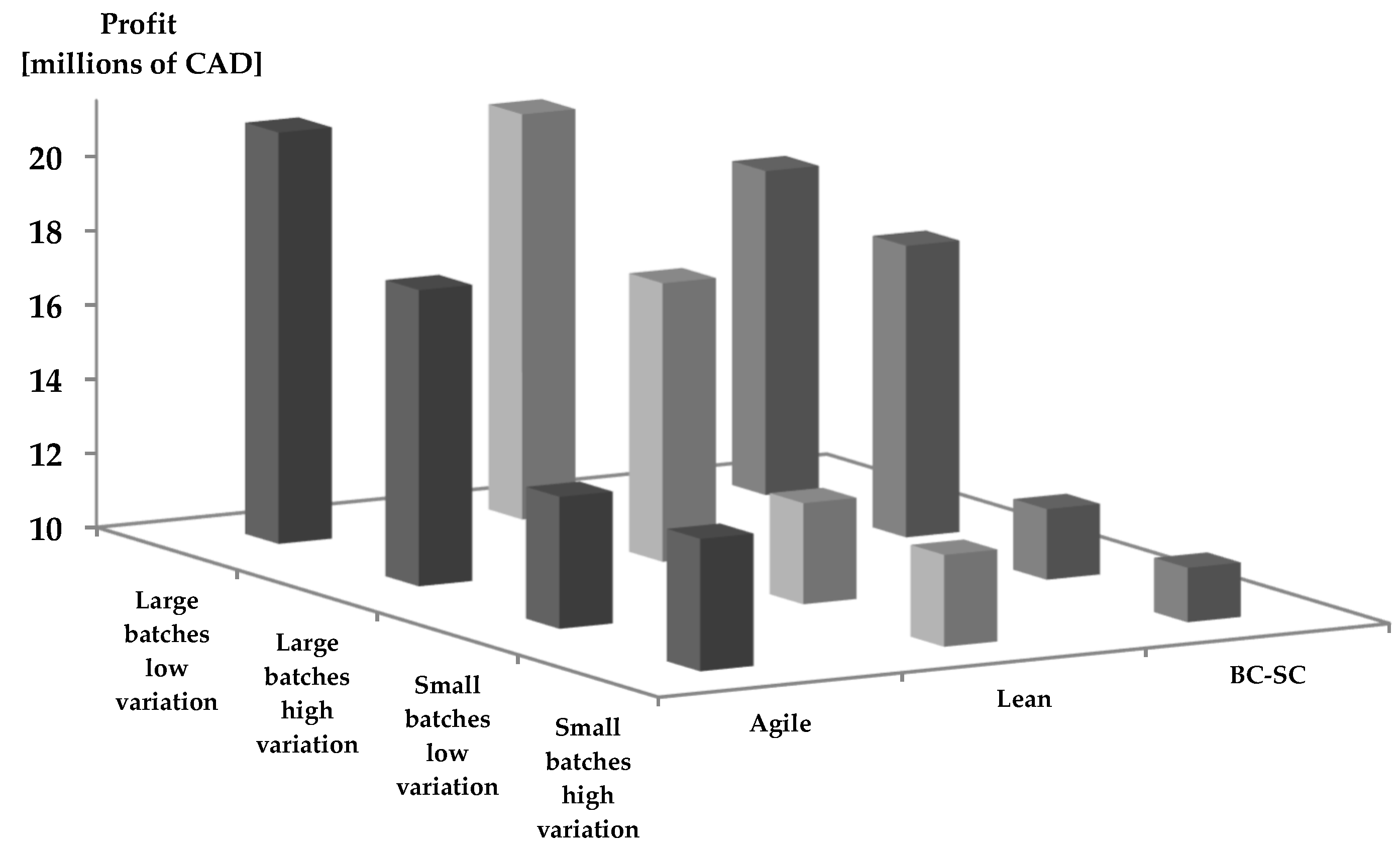
For the sake of simplicity, the averages of the optimization models’ economic outcomes were aggregated by: manufacturing environment, batch sizes, and demand variation inside the batch. Incomes for the lumber demand scenarios were similar; however, operation costs guided by manufacturing drivers determined different profit and performances (see

Table A8. Summary of economics by lumber demand scenario (LDS) and manufacturing environment (ME) (in millions of CAD).

LDS	Base			Large Batches Low Variation			Large Batches High Variation			Small Batches Low Variation			Small Batches High Variation
ME	Agile	Hybrid	Lean	Agile	Hybrid	Lean	Agile	Hybrid	Lean	Agile	Hybrid	Lean	Agile	Hybrid	Lean
Profit	19,671	20,402	18,869	21,084	18,736	20,921	17,976	17,857	17,505	13,550	11,904	12,721	13,562	11,465	12,471
Incomes	34,264	34,443	33,454	42,977	43,155	42,184	29,763	29,949	29,013	18,368	18,635	18,437	17,842	18,074	17,961
Procurement cost	10,643	11,821	10,326	14,879	18,993	15,291	8938	8577	7920	3080	5999	4743	2607	5983	4864
Manufacturing cost	2226	2574	2187	2899	3205	2902	2035	2357	1826	1299	1717	1340	1181	1573	1323
Over-below cap. Cost	15	14	11	28	21	11	11	15	11	4	8	13	5	11	13
Penalized incomes	121	1068	0	468	798	915	311	1189	70	210	1147	897	182	1186	1090
Penalty cost	1830	1034	2061	4555	2903	3975	1114	316	1821	644	0	516	671	0	380
All cost	14,714	15,442	14,585	22,361	25,122	22,179	12,098	11,265	11,578	5028	7724	6613	4463	7566	6579
Variation (%)	0%	−5%	1%	0%	−11%	−1%	0%	−1%	−3%	0%	−12%	−6%	0%	−15%	−8%

, and Figure 2). A descriptive results analysis per ME and LDS follows.

Results for MEs

On average, the agile approach was the most profitable approach, followed by lean (3.9% below agile) and BC-SC (6.4% below agile). Regardless of the variation, for large batches, agile was still the most profitable, followed by lean (1.6% below agile) and BC-SC (6.3% below agile). For large batches with low variation, the agile and lean approaches obtained almost equal profits, followed by BC-SC (11.1% below agile and lean). For high variation, agile and lean profits were almost equal, followed closely by BC-SC (2.6% below lean and agile). Regardless of the variation, the differences were larger for small batches than for large batches, where the agile approach remained the most profitable, followed by the lean (7.1% below) and BC-SC (13.8% below) approaches. For small batches with low variation, agile still produced the highest profits, followed by the lean (6.1% below) approach and then the BC-SC (12.1% below) approach. For high variation, the differences were larger, with agile being the most profitable, followed by lean (8.0% below) and then BC-SC (15.5% below).

The agile approach led to lower harvest levels, followed by the lean and BC-SC approaches. The timber volume supplied to the sawmill followed the same trend. As a consequence, procurement and manufacturing costs followed the same order, and because the lumber demand data were the same in each LDS, incomes were similar for the agile, lean, and BC-SC approaches, although the BC-SC and lean approaches had higher costs. Over and under-capacity costs were not significant due to the low allowable capacity deviation between periods.

In our formulations, overproduction was paid for with lower prices, while underproduction was penalized by charging a cost for the underproduction, which was determined by multiplying the volume of underproduction by a fraction of the lumber price. This mechanism was efficient at controlling production, and brought flexibility that was translated to a customer service emphasis in all of the approaches. The agile approach had the smallest magnitude of lumber over and underproduction, with the exception of large batches with low variation. Lumber production was mostly below lumber demand. The lean approach produced large volumes over and under the demand for most of the small and large batches. The BC-SC approach produced large over-demand volumes for most of the small and large batches, with the exception of large batches with low variation.

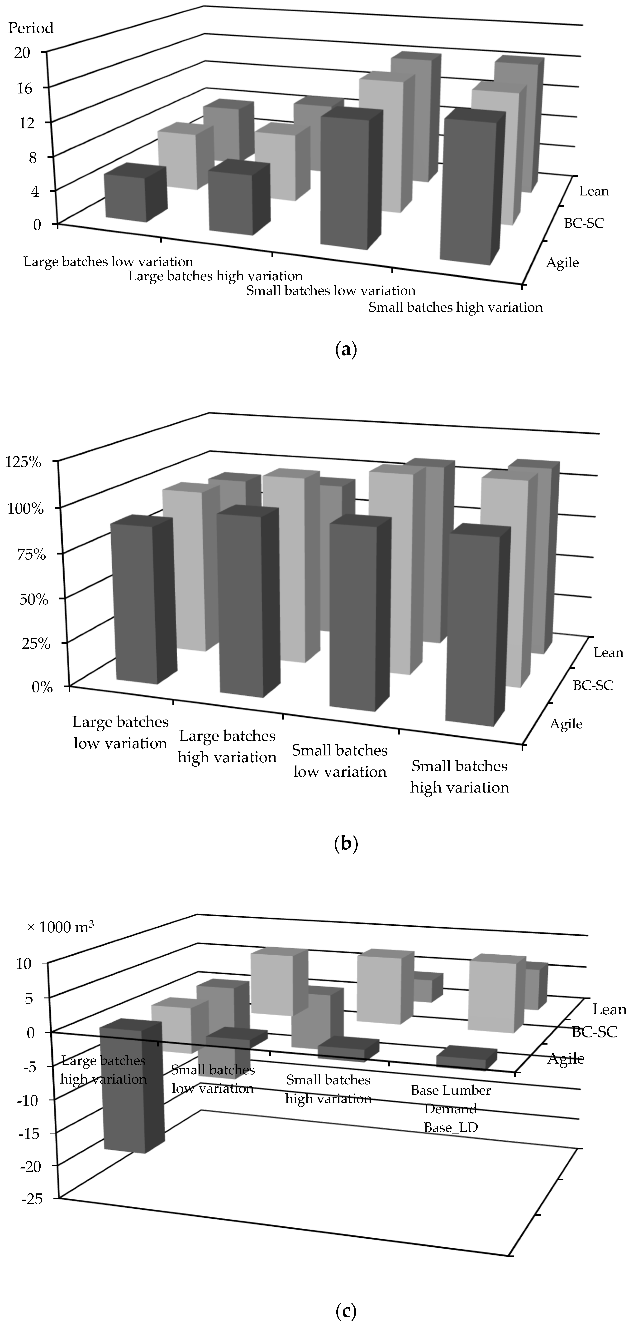
In terms of order fulfillment, the agile approach led to production levels being as close as possible to demand, with 89%, 99%, 99%, and 98% of demand met by production for large batches with low and high variation and small batches with low and high variation, respectively. For the lean approach, order fulfillment was less stable, with 91% and 92% of demand met by production for large batches with low and high variation, respectively, and 107% and 111% of demand met by production for small batches with low and high variation, respectively. The BC-SC approach produced over the demand most of the time, with 96% and 108% of demand met by production for large batches with low and high variation, respectively, and 114% and 115% of demand met by production for small batches with low and high variation, respectively. Consequently, BC-SC was the worst at controlling lumber production. The flow time indicates the degree of responsiveness; thus, on average, the agile approach showed 10.4 periods; the BC-SC approach showed 11.7 periods, and the lean approach showed 12.2 periods of flow time. These results agree with Narasimhan et al. [26], who found higher delivery speeds and reliability for the agile approach compared with the lean approach (Figure 3, Table A8 and

Table A9. Supply chain performance metrics by lumber demand scenario (LDS) and manufacturing environment (ME).

SC Performance Indicator	Flow Time (Periods)			Orders Fulfillment (%)			Over-Under Lumber Production (m3)
ME/LDS	Agile	Hybrid	Lean	Agile	Hybrid	Lean	Agile	Hybrid	Lean
Large batches low variation	5.26	7.19	7.53	89%	96%	91%	(18,393)	(7184)	(15,417)
Large batches high variation	6.98	8.28	8.98	99%	108%	92%	(1253)	9100	(9073)
Small batches low variation	14.28	15.75	15.95	99%	114%	107%	(1756)	9744	3515
Small batches high variation	15.14	15.45	16.28	98%	115%	111%	(1534)	10,258	6222
Base lumber demand	5.73	6.19	8.14	94%	103%	91%	(7409)	3993	(11,170)

in the Appendix B).

4. Discussion

The industrial relevance of lean, agile, and hybrid manufacturing systems is clear, but there is a need to unpack these ambiguous terms, if integration of these conflicting paradigms is to be logically developed to meet specific business needs [27]. An analysis and discussion of tradeoffs based on variation, inventory, and capacity follows.

Our results can be compared with Goldsby et al. [1] with respect to the economic performance of MEs, although they used DES and we used MIP to model the SC. Nevertheless, both analyses determined the operational costs. The lowest costs were produced by the agile approach, followed by the lean approach (5% over) and the BC-SC approach (14% over). However, Goldsby et al. [1] showed only a small difference between the lean and agile costs (e.g., only 2%) and a hybrid with 15% higher costs. Although the differences in percentages between our costs were larger, both results are close in terms of magnitudes and trends. Furthermore, we found that the operational costs agree with the results of [Narasimhan et al. [26], in which lean costs were the lowest, closely followed by agile costs. Goldsby et al. [1] analyzed the concept of the “order-to-ship time” as a customer service parameter. Also, Qrunfleh et al. [28] explored the ability of lean and agile systems to increase responsiveness and waste elimination. They found that an agile SC strategy contributes significantly to building SC responsiveness. Contrarily, no significant relationship between a lean SC strategy and SC chain responsiveness was found. However, a lean SC strategy has a significant relationship with waste elimination. In our study, we did not explicitly model delivery time, although order fulfillment or over/under production attempts to capture this. They stated that lean exhibits three times lower order-to-ship times than the hybrid (i.e., BC-SC) approach and eight times slower order-to-ship times compared to the agile approach, without mentioning backorder numbers. We considered customer service parameters as order fulfillments, as did Babazadeh et al. [7]. Nevertheless, our results show that the lean approach produced double the number of backorders of agile, which agrees with the results of Narasimhan et al. [26] and Enriquez et al. [29], which showed higher delivery speeds and delivery reliability for the agile approach over the lean approach. These experimental results are in great tuning with manager perceptions, which strongly believes that lean SC strategy is mostly focused on waste elimination rather that responsiveness improvement; this is the capital emphasis of agile SC strategy [28].

The lean supply paradigms perform better with a low variation of products enabling flow, and reducing the need for buffer or protective inventory and capacity. However, with the growth in products innovation and demand uncertainty, supply chains need to strategically locate inventory and capacity to enable the flow of production [27]. However, our results indicate that lean accumulates more inventories than agile. Also, Goldsby et al. [1] found more inventory in agile than in hybrid, but we found the opposite. The differences in inventory can be related to our over and under-demand lumber production constraints, which cannot be stated in a DES model as explicitly as in an MIP model. There are also ship-to-order and order fulfillment conceptual differences between the studies. However, our results for the order fulfillment, overproduction, and underproduction of lumber and inventory are in agreement with the results of Hallgren et al. [2], which showed that the lean approach had a significant impact on cost efficiency, while the agile approach did not. However, the agile approach had a higher delivery performance (e.g., order fulfillment).

In an effort to measure the impacts of demand variation and batch size, we tested the impact of lumber demand scenarios on MEs. Unfortunately, we found a few quantitative and theoretical research to compare with, so we can only benchmark our results with them. Our results show that the agile approach has the highest profit, closely followed by the lean and BC-SC approaches. Goldsby et al. [1] showed that the agile and lean approaches were equally cost-efficient, while the hybrid approach was by far the most expensive (the most cost-efficient ME was assumed to be the one with highest profits). Enriquez et al. [29] found that the agile system is more attractive when one of the demands is low and there is a high variation of demands, which is equivalent to small batches with high variation in our study. Our results showed that the agile and lean approaches continued to have higher profits than the BC-SC approach for large batches without considering the effect of demand variation. When lumber demand showed low variation, no change was observed between the agile and lean profits, while the profits of BC-SC decreased by half. These profits are comparable to those identified by Christopher et al. [6]. While the lean approach was expected to have higher profitability than the agile approach for this type of lumber demand, instead it showed the same costs as the agile approach. However, when lumber demand shows high variation, differences in profits were tiny, with the agile and BC-SC approach were leading profits, followed closely by the lean approach. These profits are in agreement with those of Christopher et al. [6]. The BC-SC approach had the highest profits for product demands characterized by high variation and high volumes.

For small batches, the agile approach had higher profits than the lean and BC-SC approaches, but with larger profit differences. Our results for high variation again agreed with those of Christopher et al. [6], who stated that “agile profitably responds to high variety and low volumes”. However, for low variation, my results did not show that the BC-SC approach had a higher profit as Christopher et al. [6] suggested, probably because we did not explicitly work with mixed portfolios of demands, where the hybrid approach is supposed to perform better.

In compliance with the economic penalties used for over and under-demand and capacity usage deviations, the agile approach always showed lower costs than the lean approach, which was able to use more capacity and deviate farther from demand, while compromising costs. The BC-SC approach showed the highest costs because log demand was a forecasted average per period and was not exactly the required log demand. As a consequence, order fulfillment (%) and lumber production deviations were higher than they were in the lean and agile approaches, where timber was pulled directly from sawmills every period.

The models determined the expected result patterns with an objective function as a central driver plus constraints as second order drivers. Although Al-Aomar et al. [8] claimed that lean objectives are in conflict and a multi-objective formulation is required, we showed that ME attributes, such as customer service, chase and level manufacturing strategies, can be modeled with MIP, as Babazadeh et al. [7] did when modeling the design of an agile SC. Alternatively, if agile, lean, and hybrid approaches are required to be measured in the short term, their stochastic shop floor techniques could be modeled with DES and VSM, and multi-objective techniques.

Lumber production outsourcing, interchanges of lumber between sawmills, over/under capacity usage, and over/under demand features increase the ability of our formulations to represent MEs. Although over/underproduction capacity usage penalties did not play a large role in costs, because their related constraints were too tight, these constraints actively helped to model chase and level manufacturing strategies. However, over/under demand lumber production constraints played a large role in relaxing and controlling order fulfillment and in controlling lumber production, which is another central feature of MEs [16].

For SC practitioners, the results of this research highlight the benefits that forest firms can capitalize if they consider the introduction of lean, agile, and hybrid SC strategies. However, SC managers should be aware of the nature of the lumber products demand before choosing any of them. Another aspect that should be kept in mind is that the type of SC can capitalize the benefits of the lean agile appraoch, and hybrid (leagile) manufacturing [30]. The ability of these managerial tools to improve SC performance has been identified. Business units containing corporate headquarters, sales and services groups, inventory and management groups, and production units are the SCs with higher advantages. Furthermore, there are other SC concepts that were not included in this research as postponement or supplier partnerships [28], which could add extra criteria for SC strategy selection.

5. Conclusions

Our research shows that MEs for the case studies can be modeled with a reasonable level of detail with MIP, and that these formulations react to the lumber demand scenarios, as stated in our objectives. Indeed, our results highlight how manufacturing drivers and demand attributes influence the economic performance of lean, hybrid, and agile approaches for the forest-to-lumber SC.

When suggesting that ME should be adopted for the particular case of integrated BC coastal forest-to-lumber SCs, the attributes of demand should be considered. When lumber demand is stable with low variation and large volumes, agile or lean principles should be adopted. However, when lumber demand is unstable with high variation and large volumes, hybrid or agile principles should be maintained. When lumber demand is unstable with high variation and small volumes, an agile approach clearly provides higher profits than any other ME. For the same conditions of lumber demand, but with low variation, the agile approach is recommended; however, further analysis is required, because a hybrid (i.e., BC-SC) approach is in theory supposed to be the most appropriate under these circumstances.

There is an opportunity to increase profits by 11.1% by adopting an agile approach when lumber demand is stable with low variation and large volumes. However, the opportunity for increased profits is zero under the same demand attributes, but with high variation. Contrarily, there is an opportunity to increase profits by 12.1% by adopting agile or lean approaches when lumber demand is stable with low variation and small volumes, and there is an opportunity to increase profits by 15.5% when lumber demand is unstable with high variation and small volumes. However, these profit increments are subject to over/under capacity and demand penalties, the lumber demand scenarios, and the exploratory nature of this work. These results are specific to our case studies and the over/under demand and production penalties we used.

References

- Goldsby, T.; Griffis, S.; Roath, A. Modeling lean, agile and leagile supply chain strategies. J. Bus. Logist. 2006, 27, 57–80. [Google Scholar] [CrossRef]
- Hallgren, M.; Olhager, J. Lean and agile manufacturing: External and internal drivers and performance outcomes. Int. J. Oper. Prod. Manag. 2009, 29, 976–999. [Google Scholar] [CrossRef]
- Naylor, B.; Nain, M.; Berry, D. Leagility: Integrating the lean and agile manufacturing paradigms in the total supply chain. Int. J. Prod. Econ. 1999, 62, 107–118. [Google Scholar] [CrossRef] [Green Version]
- Gunasekaran, A. Agile manufacturing: A framework for research and development. Int. J. Prod. Econ. 1999, 62, 87–105. [Google Scholar] [CrossRef] [Green Version]
- Chopra, S.; Meindl, P. Supply Chain Management: Strategy, Planning and Operation, 1st ed.; Prentice Hall College Division: Englewood, NJ, USA, 2000. [Google Scholar]
- Christopher, M. The Agile Supply Chain Competing in Volatile Markets. Ind. Mark. Manag. 2000, 29, 37–44. [Google Scholar] [CrossRef] [Green Version]
- Babazadeh, R.; Razni, J.; Ghodsi, R. Supply chain network design problem for a new market opportunity in an agile manufacturing system. J. Ind. Eng. Int. 2012, 8, 8–19. [Google Scholar] [CrossRef] [Green Version]
- Al-Aomar, R. Handling multi-lean measures with simulation and simulating annealing. J. Frankl. Int. 2011, 348, 1506–1522. [Google Scholar] [CrossRef]
- Huang, S.; Uppal, M.; Shi, F. A products driven approach to manufacturing supply chain selection. Supply Chain Manag. Int. J. 2002, 7, 189–199. [Google Scholar] [CrossRef]
- Sipper, D.; Bulfin, R. Production Planning, Control, and Integration; McGraw-Hill: New York, NY, USA, 1997. [Google Scholar]
- Hege, L.; Gicquel, C.; Minoux, M. Lagrangian Relaxation for Multi-Level Lotsizing Problems; ROADEF: Toulouse, France, 2010. [Google Scholar]
- Billington, P.J.; McClain, J.O.; Thomas, L.J. Mathematical programming approaches to capacity-constrained MRP systems: Review, formulation and problem reduction. Manag. Sci. 1983, 29, 1126–1141. [Google Scholar] [CrossRef]
- Hung, Y.F.; Chien, K.L. A multi-class multi-level capacitated lot sizing model. J. Oper. Res. Soc. 2000, 51, 1309–1318. [Google Scholar] [CrossRef]
- Yang-Hua, L.; van Landeghem, H. An application of simulations and value stream mapping in lean manufacturing. Presented at the 14th European Simulation Symposium, Dresden, Germany, 23–26 October 2002. [Google Scholar]
- Aldulmalek, F.; Rajgopal, J. Analyzing the benefits of lean manufacturing and value stream mapping via simulation: A process sector case study. Int. J. Prod. Econ. 2007, 107, 223–236. [Google Scholar] [CrossRef]
- Paine, T.; Peters, M.J. What is the right supply chain for your products? Int. J. Logist. Manag. 2004, 15, 77–92. [Google Scholar] [CrossRef]
- Mason-Jones, R.; Naim, M.M.; Towill, D.R. The impact of pipeline control on supply chain dynamics. Int. J. Logist. Manag. 1997, 8, 47–62. [Google Scholar] [CrossRef]
- Mason-Jones, R.; Towill, D.R. Using the information decoupling point to improve supply chain performance. Int. J. Logist. Manag. 1999, 10, 13–26. [Google Scholar] [CrossRef]
- Bruce, M.; Dayl, L. Lean or agile, a solution for supply chain management in the textiles and clothing industry? Int. J. Oper. Prod. Manag. 2004, 24, 151–170. [Google Scholar] [CrossRef]
- Christopher, M.; Towill, D. An integrated model for the design of agile supply chains. Int. J. Phys. Distrib. Logist. Manag. 2001, 31, 235–246. [Google Scholar] [CrossRef] [Green Version]
- Carvalho, H.; Barroso, A.P.; Machado, V.H.; Azevedo, S.; Cruz-Machado, V. Supply chain redesign for resilence using simulation. Comput. Ind. Eng. 2012, 62, 329–341. [Google Scholar] [CrossRef]
- Haartveit, E.; Kozak, R.; Maness, T. Supply chain management mapping for the forest products industry: Three cases from western Canada. J. For. Prod. Bus. Res. 2004, 1, 1–30. [Google Scholar]
- Salehirad, N.; Sowlati, T. Performance of primary wood producers in British Columbia using data envelopment analysis. Can. J. For. Res. 2005, 34, 285–294. [Google Scholar] [CrossRef]
- Western Forest Products Inc. 2010, 2011, and 2012, Annual Information Form. Available online: http://www.westernforest.com/ (accessed on the 8 October 2013).
- Agarwal, A.; Shankar, R.; Tiwari, M.K. Modeling the metrics of lean, agile and leagile supply chain: An ANP-based approach. Eur. J. Oper. Res. 2006, 173, 211–225. [Google Scholar] [CrossRef]
- Narasimhan, R.; Swink, M.; Kim, S.W. Disentangling leanness and agility: An empirical investigation. J. Oper. Manag. 2006, 24, 440–457. [Google Scholar] [CrossRef]
- Stratton, R.; Warburton, R.D.H. The strategic integration of agile and lean supply. Int. J. Prod. Econ. 2003, 85, 183–198. [Google Scholar] [CrossRef] [Green Version]
- Qrunfleh, S.; Tarafdar, T. Lean and agile supply chain strategies and supply chain responsiveness: The role of strategic supplier partnership and postponement. Supply Chain Manag. Int. J. 2013, 18, 571–582. [Google Scholar] [CrossRef]
- Enriquez, N.S.; Haw, J.I.; Tam, K.E.; Cruz, D.E. A Supply Chain Model for Lean Facilities Considering Milk Round Replenishment, Postponement Production System and One-For-One Base Stock Inventory Policy Decision. In Proceedings of the 2011 International Conference on Industrial Engineering and Operations Management (IEOM), Kuala Lumpur, Malaysia, 22–24 January 2011; pp. 500–504. [Google Scholar]
- Krishnamurthy, R.; Yauch, C.A. Leagile manufacturing: A proposed corporate infrastructure. Int. J. Oper. Prod. Manag. 2007, 27, 588–604. [Google Scholar] [CrossRef]
Figure 1.
Forest to lumber British Columbia (BC) coastal supply chain case study.
Figure 2.
Profits variation between MEs and lumber demand scenarios (LDSs).
Figure 3.
Flexibility parameters by ME and LDS, which should be listed as: (a) Flow time (periods), (b) Orders fulfillment (%), and (c) Over–under lumber production × 1000 m3).