Broadening Understanding on Managing the Communication Infrastructure in Vehicular Networks: Customizing the Coverage Using the Delta Network

Abstract

Over the past few decades, the growth of the urban population has been remarkable. Nowadays, 50% of the population lives in urban areas, and forecasts point that by 2050 this number will reach 70%. Today, 64% of all travel made is within urban environments and the total amount of urban kilometers traveled is expected to triple by 2050. Thus, seeking novel solutions for urban mobility becomes paramount for 21st century society. In this work, we discuss the performance of vehicular networks. We consider the metric Delta Network. The Delta Network characterizes the connectivity of the vehicular network through the percentage of travel time in which vehicles are connected to roadside units. This article reviews the concept of the Delta Network and extends its study through the presentation of a general heuristic based on the definition of scores to identify the areas of the road network that should receive coverage. After defining the general heuristic, we show how small changes in the score computation can generate very distinct (and interesting) patterns of coverage, each one suited to a given scenario. In order to exemplify such behavior, we propose three deployment strategies based on simply changing the computation of scores. We compare the proposed strategies to the intuitive strategy of allocating communication units at the most popular zones of the road network. Experiments show that the strategies derived from the general heuristic provide higher coverage than the intuitive strategy when using the same number of communication devices. Moreover, the resulting pattern of coverage is very interesting, with roadside units deployed a circle pattern around the traffic epicenter.

1. Introduction

Smart cities are receiving increasing attention from governments and society. Washburn et al. [1] define smart cities as “the use of smart computing technologies to make the critical infrastructure components and services of a city—which include city administration, education, healthcare, public safety, real estate, transportation, and utilities—more inteligent”. Nam and Pardo [2] group key conceptual components of smart cities into three categories of core factors: Technology (infrastructures of hardware and software), people (creativity, diversity, and education), and institution (governance and policy). Given the connection between the factors, a city is smart when investments in human/social capital and IT infrastructure fuel sustainable growth and enhance a quality of life, through participatory governance [3].

Over the past few decades, the growth of the urban population has been remarkable. Nowadays, 50% of the population lives in urban areas, and forecasts point that by 2050 this number will reach 70%. Today, 64% of all travel made is within urban environments and the total amount of urban kilometers traveled is expected to triple by 2050 [4]. Thus, seeking novel solutions for urban mobility becomes paramount for 21st century society. In fact, several researches are already in advanced state: The development of autonomous vehicles [5] combined with car-sharing services [6] may shape a new automotive industry, and introduce a new paradigm in the way we use vehicles. In a few decades, cars tend to turn into services, rather than properties. Users would simply pay-per-use, instead of buying vehicles. Such change would drastically reduce the demand for parking spaces, since less vehicles would be required. At the same time, the society would benefit from a better use of natural resources employed in manufacturing vehicles (which spend a considerable part of their lifetimes parked).

However, this intelligent system of urban mobility depends on the development of efficient information and communication technologies capable of providing the integration of users, vehicles, traffic lights, parking lots, traffic authorities, and all other entities involved in the traffic system [7]. Such integration can take place through, basically, three communication paradigms: (a) Cellular networks; (b) ad hoc vehicle to vehicle communication; (c) dedicated roadside infrastructure based. Most communication tends to take place through high-speed cellular networks [8,9], ideal for commercial and third-party applications addressing real-time driver interaction [10], routes planning [11], vehicle tracking [12], monitoring driving style [13], performance of the vehicle [14], condition of roads [15,16], driver reputation [17], network autentication [18], smart traffic lights [19], traffic monitoring [20], accident detection [21,22], and several other types of applications still to appear in the near future. Complementary, some applications tend to benefit from the direct ad hoc communication between vehicles [23], such as collision avoidance systems [24], and platooning [25], where low communication delay, reduced risk of interference, and physical proximity are key factors.

In addition to these paradigms, traffic management can also benefit from the implementation of an infrastructure-based network dedicated to vehicular communication through the deployment of communication devices in strategic locations of the road network. Such network would be responsible for routing sensitive data. Typically, these networks are managed by government, but they could also be run by private organisations, as for example through bidding. Examples of applications for these dedicated networks include traffic signal management [26], virtual traffic light implementations [27], special traffic-related communications (such as online notification of traffic penalties, lane-change maneuvers [28]), and even sending commands to vehicles (such as “reduce speed”). In fact, in a fully coordinated system, traffic authorities could even take over the vehicle in certain critical conditions, such as crossing specific intersections, in order to maximize the traffic flow efficiency. The focus of the present work is on this type of network.

However, for vehicular networks to become feasible in practice, some issues remain open, such as security and performance, as e.g., network coverage and connectivity. Vehicular networks are characterized by the rapid movement of vehicles along the road network, making connectivity dependent on location. In this work, we go deeper into the study of the Delta Network [29]. The Delta Network characterizes the connectivity of the vehicular network through the percentage of travel time in which vehicles are connected to roadside units. In summary, this article reviews the concept of the Delta Network and extends its study through the presentation of a general heuristic based on the definition of scores to identify areas of the road network that should receive coverage.

The definition of the score is based on the number of vehicles meeting coverage in relation to the distance traveled, and different score definitions lead to different roadside units deployment strategies. After defining the general heuristic, we show how small changes in the score computation can generate very distinct (and interesting) patterns of coverage, each one suited to a given scenario. In order to exemplify such behavior, we propose three deployment strategies based on simply changing the computation of scores.

This work is organized as follows: Section 2 overviews a representative set of related work. Section 3 introduces the Delta Network, and discusses how to solve the allocation of roadside units for achieving one single performance target. Section 4 extends our analysis on the Delta Network in order to achieve global solutions using the concept of scores. Section 5 presents experiments illustrating aspects discussed in the previous sections. Section 6 concludes the work.

2. Related Work

Connected vehicles are gaining increasing visibility. Weeratunga and Somers [30] present an extensive discussion on the future of connected vehicles. Authors notice that “...rapid technological developments are occurring within two separate areas defined as Automated Vehicles and Connected Vehicles. The development of connected vehicles and automated vehicles is occurring largely independently, although convergence of the two areas will be required for full automation of vehicles”.Lu et al. [31] notices that connected vehicles are expected to be the next frontier for automotive revolution and the key to the evolution to next generation intelligent transportation systems. Authors focus on wireless technologies and potential challenges to provide vehicle-to-x connectivity, discussing challenges and reviewing the state-of-the-art wireless solutions for vehicle-to-sensor, vehicle-to-vehicle, vehicle-to-Internet, and vehicle-to-road infrastructure connectivities. Vehicular communication has been extensively studied. A comprehensive survey on infrastructure-based vehicular networks is presented in works [7,23]. Along this section, we overview a representative list of selected works in data dissemination, data scheduling, communication protocols, and deployment strategies.

Data dissemination is at the core of most services enabled by vehicular networks. Sanguesa et al. [32] present the review of 23 different kinds of dissemination schemes highlighting the benefits and drawbacks associated with each one. Kai and Lee [33] propose push-based broadcast data dissemination in heavy traffic: messages are periodically broadcasted to passing vehicles. In light traffic scenarios, vehicles query on-demand for traffic information. Authors derive a mathematical model that shows the effectiveness of the solution and they conclude that data dissemination in vehicular networks should be adaptable to dynamic traffic environments. Bruno and Nurchis [34] assume vehicles equipped with cameras and the problem is how to deliver the images to remote data collectors. Authors propose a data collection algorithm capable of eliminating the redundancy of data transmitted by moving vehicles. In a real situation, several vehicles may report the same event. Thus, data redundancy mitigation is necessary to improve the network efficiency. Dighriri et al. [8] propose a novel data traffic aggregation and slicing model with algorithms in 5G uplink, based on classifying and measuring the data traffic to achieve quality of service for smart systems.

Data scheduling is also addressed. Shumao et al. [35] propose a downlink scheduler to deliver high-quality video-on-demand over infrastructure-based vehicular networks. The scheduler is deployed in roadside units to coordinate the transmission of packets according to the importance of packet to video quality, the playback deadline, and also real-time information of vehicles. Zhang et al. [36] also devise a scheduling algorithm to coordinate the distribution of data files in vehicular networks. A collection of data files is stored at distributed locations and delivered to passing vehicles. According to the popularity of files, the proposed algorithm schedules the location of files through the selective upload and download of roadside units to maximize the delivery ratio of files to vehicles. Complimentary, Dighriri et al. [37] propose data traffic slicing model along with the comparison of packet traffic scheduling mechanisms such as weighted fair queuing, priority queuing, and first-in-first-out in the 5G mobile network.

Communication protocols have also been proposed. Baker et al. [38] propose a GreeDi based reactive routing protocol aimed at selecting the most efficient route in terms of energy consumption between two nodes in VANETs. Korkmaz et al. [39] propose a cross-Layer multi-hop data delivery protocol with fairness guarantees where vehicles do not communicate with roadside units individually, but through one leader. The goal is to reduce the network traffic and to use bandwidth more efficiently. The leader will collect all information from other nodes and share it with roadside units. Complementary, Hadaller et al. [40] propose a protocol to increase the global data transfer. Authors observe that when roadside units are shared by more than one vehicle, the vehicle with the lowest transmission rate reduces the effective transmission rate of all other vehicles. Observing that every vehicle eventually receives good performance when it is near the roadside unit, the authors propose a medium access protocol that opportunistically grants access to vehicles with maximum transmission rate. The overall system throughput is improved by a factor of four.

Deployment based on the V2I contact probability is addressed by Bazzi et al. [41]. Authors discuss the system design and address the cellular offloading issue in urban scenarios through the deployment of WAVE/IEEE 802.11p devices on vehicles and roadside units. The work shows the impact of the percentage of equipped vehicles, of the number of deployed roadside units, and of the adopted routing protocols on the amount of data delivered. Results, obtained through an integrated simulation platform taking both realistic vehicular environments and wireless network communication aspects into account, show that the deployment of few road side units and the use of low complexity routing protocols leads to a significant reduction of cellular resource occupation, even approaching 100% with a high density of equipped vehicles.

Deployment for content delivery is addressed in [42]. Authors present a mixed-integer quadratic programming based optimum roadside units deployment scheme to provide Internet access services for the maximum road traffic volumes with limited number of roadside units. Additionally, Silva et al. [43] investigate the application of Content Delivery Networks (CDN) to the vehicular scenario, modeling the distribution of several contents within distinct levels of QoS. Since a given content may be meaningful only to a given region of interest, they assume that each content type is related to a target region where it must be made available.

Deployment based on evolutionary approaches is proposed by Lochert et al. [44]. Authors study how the infrastructure should be used to improve data travel time over very large distances. They present a multi-layer aggregation scheme defining landmarks. Cars passing landmarks record the time travel, which is aggregated to infer the time travel between more distant landmarks. These aggregation steps are performed by the cars themselves in a completely decentralized basis. The minimal initial deployment of roadside units is handled by a genetic algorithm based on the travel time savings. Complementary, Cavalcante et al. [45] apply genetic programming to solve the deployment as a Maximum Coverage Problem.

Linear Programming Models are also considered. Aslam et al. [46] use binary integer programming to solve the allocation of roadside units. They eliminate minor roads and model major roads as a grid. Authors present two different optimization methods for placement of a limited number of roadside units in an urban region: (a) Analytical Binary Integer Programming (BIP); (b) novel Balloon Expansion Heuristic (BEH). The BIP method utilizes branch and bound approach to find an optimal analytical solution whereas BEH method uses balloon expansion analogy to find an optimal or near optimal solution. Authors conclude that the BEH method is more versatile and performs better than BIP method in terms of the computational cost and scalability. Furthermore, Yingsi et al. [47] study the deployment of the roadside infrastructure by formulating an optimization problem and solving it using Integer Linear programming. The proposed optimization framework takes into account the effect of buildings on signal propagation, LAN lines and road topology. The formulation assumes a grid-like road network.

Modeling the deployment are a Maximum Coverage Problem is also considered. Trullols et al. [48] study the placement of the roadside units into an urban area. The authors use a realistic data set and propose modeling the placement as a Knapsack Problem (KP) and also as a Maximum Coverage Problem (MCP-g). The heuristic MCP-g models the deployment of roadside units as a maximum coverage problem, and assumes previously knowledge of all vehicles trajectories. Complimentary, when we intend to maximize the number of distinct vehicles contacting the infrastructure without identifying individual vehicles, we may rely on migration ratios of vehicles between adjacent locations of the road network as presented in [49].

Analytic studies are also found in the literature. Bazzi et al. [50] address cellular systems as the most feasible solution in the short term to collect information messages from vehicles to a remote control center. The paper proposes a mathematical model to evaluate the impact of the envisioned service on cellular systems capacity and coverage in simplified scenarios. Results show that the acquisition of small and frequent packets from vehicles is affected by interference more than other services, such as the voice service.

Finally, the work presented by Zizhan et al. [51] serves as inspiration for the Delta Network reviewed in Section 3. Authors propose Alpha Coverage to provide worst-case guarantees on the interconnection gap measured in terms of traveled distance. A deployment of roadside units is considered $\alpha$-covered if any path of length $\alpha$ on the road network meets at least one roadside unit.

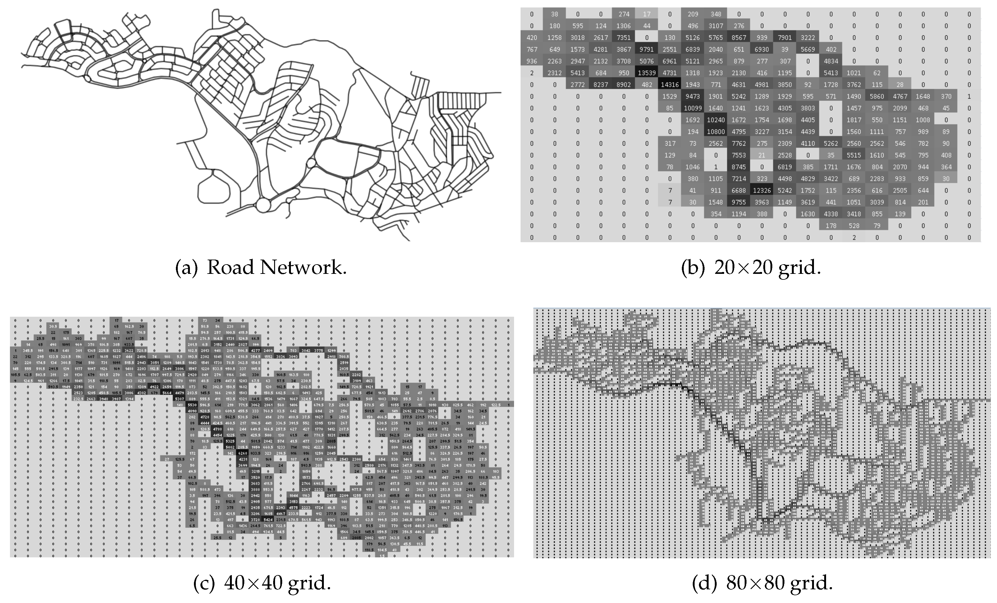
3. Delta Network: Measuring the Network Performance Using the Relation between the Connected Time and Trip Duration

Measuring the connected time is a way of characterizing vehicular networks based on the QoS experienced by users. Users receiving more connection tend to receive higher QoS by the network. Hence, measuring the connection time proportionally to the distance traveled by vehicles seems an interesting way of characterizing vehicular networks. Such measurement is given by the Delta Network [29]. Delta measures the connection time according to the trip duration, and we express it as ${\Delta }_{{\rho }_2}^{{\rho }_1}$. Parameter ${\rho }_1$ represents the connection duration factor. For instance, should vehicles be connected during 5% of the trip, then ${\rho }_1$ must be 0.05. Complementary, ${\rho }_2$ indicates the share of vehicles experiencing the connection duration defined by ${\rho }_1$. Thus, a vehicular network is ${\Delta }_{{\rho }_2}^{{\rho }_1}$ whenever ${\rho }_2$ percent of vehicles experience connection during ${\rho }_1$ percent of the trip duration.

Figure 1 illustrates the Delta metric. The metric is not represented by a single value. Instead, the Delta Network is represented as a curve in a 2D plan. The x-axis indicates ${\rho }_1$ (percentage of trip under coverage), while the y-axis indicates ${\rho }_2$ (share of vehicles). In fact, Delta is the relation between ${\rho }_1$ and ${\rho }_2$. The shadowed area indicates possible service levels for the network. The maximum achievable performance is indicated by the border of the curve. Complementary, outside the curve we have service levels unable to be achieved by the current network setup. Representing Delta as the relation between ${\rho }_1$ and ${\rho }_2$ has the advantage of delimiting the entire range of network operation. Such representation allows us to compare the operation of distinct vehicular networks in order to identify successful design strategies. In fact, we can use the Delta network to measure one dimension of the performance of the vehicular network (connected time in terms of trip duration), and also to plan a new network from scratch, or even update an existing one, using Delta to define the location of future roadside units.

The Delta Network is formally introduced in Definition 1.

Definition 1 (Deployment Δρ2ρ1)

Let R represent a given road network, and V be the set of vehicles traveling R. Let $C\subset V$ be the set of vehicles experiencing connection during, at least, ${\rho }_1$ percent of the trip duration. A deployment is ${\Delta }_{{\rho }_2}^{{\rho }_1}$ whenever $\frac{\left|C\right|}{\left|V\right|}\ge {\rho }_2$.

In addition, the Delta Network can be used to plan the vehicular network in order to meet predefined QoS levels for reaching requirements from vehicular applications that the network administrator intends to make available in the network. There is a wide range of vehicular applications already proposed in the literature, and many others still to be developed, where each application tends to demand a specific level of QoS from the vehicular network. In this sense, Delta Network can also be used to support network planning, defining the expected connectivity of vehicles in terms of their travel time.

Using the Delta Network to Reach a Specific Performance Target

In previous works [29,52], we have turned our attention on developing solutions for Delta in order to reach one single target performance. Basically, our goal was to minimize the number of roadside units in order to achieve a given combination of ${\rho }_2$ percent of vehicles connected to roadside units during ${\rho }_1$ percent of the trip duration, i.e., the optimal layout of roadside units for one single point composing the Delta curve (such as the red point in Figure 1). Solving this problem is interesting because it allows the network designer to build the network infrastructure guaranteeing such performance level in order to deploy a set of specific vehicular applications demanding the aforementioned connectivity.

Before continuing the discusson on the Delta Network, we describe a strategy for representing road networks with arbitrary topology. We model road networks as a grid-like structure. Basically, we divide the city into a set of same-sized urban cells (road partitions), as depicted in Figure 2. The dimensions of the urban cell may vary according to the desired accuracy, and the expected range of coverage of roadside units.

An Integer Linear Program formulation for this problem is presented in [52]. Since obtaning the exact solution requires too much computational effort, we can only solve small instances using this formulation. In order to solve large instances, we propose a greedy strategy named Delta-g in [53]. When we apply the Delta-g heuristic considering the Vehicular Mobility Trace of the city of Cologne Vehicular Mobility Trace of the city of Cologne, Germany, available at: http://kolntrace.project.citi-lab.fr/) [54] composed of $10,000$ seconds of traffic and $75,515$ vehicles, we obtain the following area to be covered according to pairs of ${\rho }_1$ (y-axis) and ${\rho }_2$ (x-axis).

In order obtain this result, we run the heuristic for each pair of {${\rho }_1$,${\rho }_2$} presented above. In the following section, we turn our attention to finding global solutions (instead of solutions for one single pair). Complimentary to this, we highlight that Figure 3 is an adaption of the result presented by our team in [53]. However, in [53] we present the percentage area to be covered in terms of the whole city of Cologne, while in Figure 3 we present the percentage area to be covered considering only areas presenting traffic.

4. Extending Delta Network to Global Solutions: Using Scores to Customize the Coverage

The previous section exploits solutions to solve the Delta Network considering a specific performance target given by a single tuple {${\rho }_1$,${\rho }_2$} (i.e., a single point within the curve shown in Figure 1). However, finding feasible solutions (or even, the optimal solution) for one single pair of {${\rho }_1$,${\rho }_2$} may not guarantee good connectivity for other combinations of {${\rho }_1$,${\rho }_2$}. Thus, now we focus on the main problem of this study: we consider solutions from a global perspective. We are no longer interested in optimizing the network for one single pair {${\rho }_1$,${\rho }_2$}, but we explore strategies for optimizing the Delta Network as a whole. We propose a simple greedy strategy for exploring properties of the Delta Network. As we show, slight changes in the deployment strategy lead to interesting changes in the coverage pattern of the vehicles.

Algorithm 1 presents the general greedy heuristic that is used to perform the experiments. It receives as input the trace of vehicles (T), and the number of available cells to be covered. The set of covered cells is reset. Then, for each uncovered cell, the heuristic covers the cell and re-runs the mobility trace in order to measure the connectivity of vehicles in terms of {${\rho }_1$,${\rho }_2$}. Since no cell is initially covered, the heuristic starts by covering cell [0,0] and evaluates the coverage. Then, it moves the coverage from location [0,0] to [0,1], and recomputes the coverage, and so forth, until evaluating all locations of the grid (lines 3–7). Then, it selects the cell presenting the highest score (score is measured according to the interest of the network designer, and, in this article, it is customized to create three strategies). The cell presenting the highest score is selected permanently for receiving coverage (lines 8–9). Then, the heuristic loops until selecting $\alpha$ covered cells.

The score computation (line 5) deserves special attention. In fact, in our opinion, the most interesting feature of this heuristic is the ability to customize the score. By customizing the score we have the opportunity to impose specific properties on the vehicular network, such as selecting the kind of trip that we intend to prioritize, and how connectivity is distributed across vehicles. In order to demonstrate how the score computation impacts the outcome of the heuristic, we present three strategies for computing the score: (a) Strategy balanced; (b) strategy direct; and (c) strategy inverse.

Algorithm 1  General greedy heuristic
Input:T, α;	▹ Receives the trace and number of available cells for coverage.
Output: covered_cells	▹ α covered cells.
1: covered_cells $\leftarrow \varnothing$;	▹ Clear vector holding deployed RSUs
2: while |covered_cells| $<\alpha$ do	▹ Loop until covering $\alpha$ cells
3: for each uncovered cell [x][y] in the grid do	▹ Loop for all cells without roadside units
add_cell[x][y] to set covered_cells;	▹ Temporarily cover the cell
5:  score[x][y] ←compute_score after adding cell [x][y];	▹ Compute score
6:  remove_cell [x][y] from covered_cells;	▹ uncover the cell
7: end for
8: [$x^{\prime }$][$y^{\prime }$] ←get_max_score(score[][]);	▹ Get the coordinates of the cell returning the highest score
9: add_cell[$x^{\prime }$][$y^{\prime }$] to set covered_cells;	▹ Cover the cell definitely
10: end while
11: return covered_cells;

The strategy balanced considers an uniform distribution of weights for all ranges of “percentage trip duration under coverage” (${\rho }_1$). The strategy computes the score of each cell by estimating the area underneath the Delta curve (since we rely on a greedy heuristic, the obtained area may not be optimal). Let us assume that cells {$c_1,c_2,\dots ,c_{n-1}$} are covered. Then, the score of cell $c_n$ is given by Equation (1):

$$\mathrm{score}\mathrm{of}\mathrm{cell}[c_n]\mathrm{in}\mathit{balanced}={\int }_0^{1}f\left(x\right)dx$$

(1)

where $f\left(x\right)$ indicates the Delta curve after covering cells {$c_1,c_2,\dots ,c_n$}.

On the other hand, the strategy direct assigns weight to cells directly proportional to the “percentage trip duration under coverage”, as indicated in Figure 4b. Hence, cells receive high reward when increasing the coverage of highly connected vehicles. The score is computed as the sum of the coverage received by each vehicle in terms of the percentage trip duration. Let us assume that cells {$c_1,c_2,\dots ,c_{n-1}$} are covered. Then, the score of cell $c_n$ is given by Equation (2):

$$\mathrm{score}\mathrm{of}\mathrm{cell}[c_n]\mathrm{in}\mathit{direct}=\sum ^{\forall v\in \mathrm{vehicles}}{\rho }_1\left(v\right)$$

(2)

where ${\rho }_1$(v) indicates the percentage of the trip duration that vehicle v is traveling under the coverage of roadside units after covering cells {$c_1,c_2,\dots ,c_n$}. Thus, the strategy direct represents an elitism: Vehicles experiencing high coverage tend to receive more coverage after each iteration (i.e., the strategy tries to extend the coverage of already covered vehicles). Complimentarly, strategy inverse assigns weight to cells inversely proportional to the “percentage trip duration under coverage” (${\rho }_1$). In other words, cells providing coverage to vehicles with low coverage (or no coverage at all) receive high reward.

$$\mathrm{score}\mathrm{of}\mathrm{cell}[c_n]\mathrm{in}\mathit{inverse}=\sum ^{\forall v\in \mathrm{vehicles}}(1-{\rho }_1\left(v\right))$$

(3)

where ${\rho }_1$(v) indicates the percentage of the trip duration that vehicle v is traveling under the coverage of roadside units after covering cells {$c_1,c_2,\dots ,c_n$}.

Figure 4 shows the distribution of weights used for computing the score. The score indicates the next cell to be covered by Algorithm 1. Figure 4a shows the distribution used by the strategy balanced. In this distribution, all ranges of “percentage trip duration under coverage” (${\rho }_1$) receive the same weight (shown in the x-axis), and the strategy tries to maximize the area under the Delta curve. Figure 4b shows the distribution used by the strategy direct, where weights are directly proportional to ${\rho }_1$. By using such distribution, we intend to increase the share of highly connected vehicles. Figure 4c shows the distribution used by the strategy inverse, where weights are inversely proportional to ${\rho }_1$.

5. Methods and Materials

Now, we present a set of experiments designed to characterize the performance of the balanced, direct, and inverse strategies. As baseline, we consider the intuitive strategy of covering locations following the order of popularity. Most popular cell gets covered first. We refer to this strategy as dl (densest locations). It receives as input the volume of traffic per cell (V), and the number of cells to be covered, returning the set of $\alpha$ cells presenting higher volume of traffic, as presented in Algorithm 2.

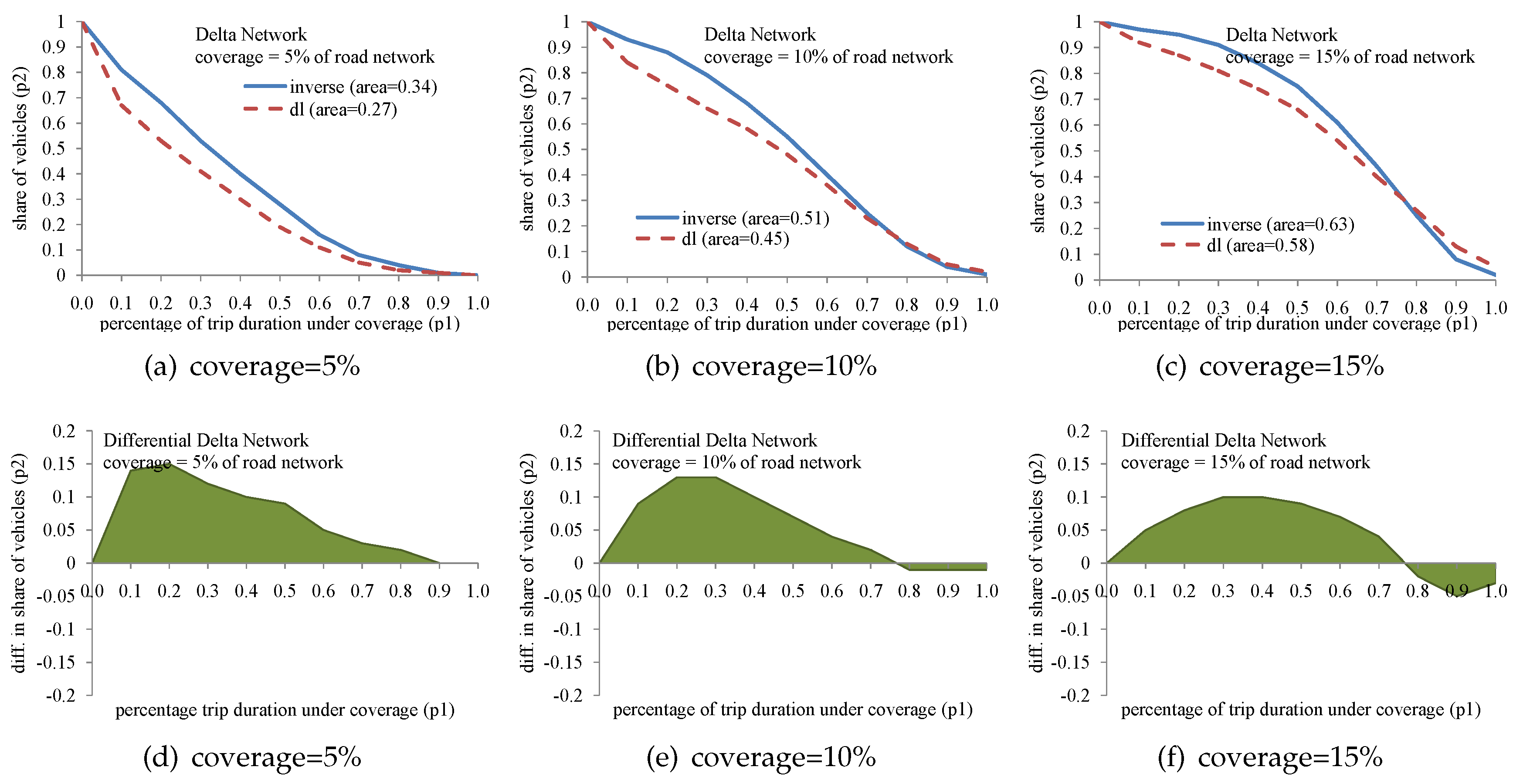
Algorithm 2 Strategy dl: Covering the most popular cells firstly.
Input:V, α;
Output: Y;	▹ Cells to be covered
1: $V^{\prime }\leftarrow$ sort(V);	▹ Sort cells according to volume of traffic
2: Y$\leftarrow$ get_initial_elements($V^{\prime }$,$\alpha$);	▹ Gets the $\alpha$ initial elements of $V^{\prime }$
3: return Y;

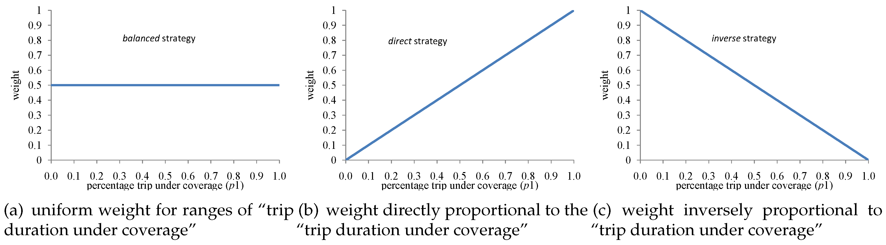
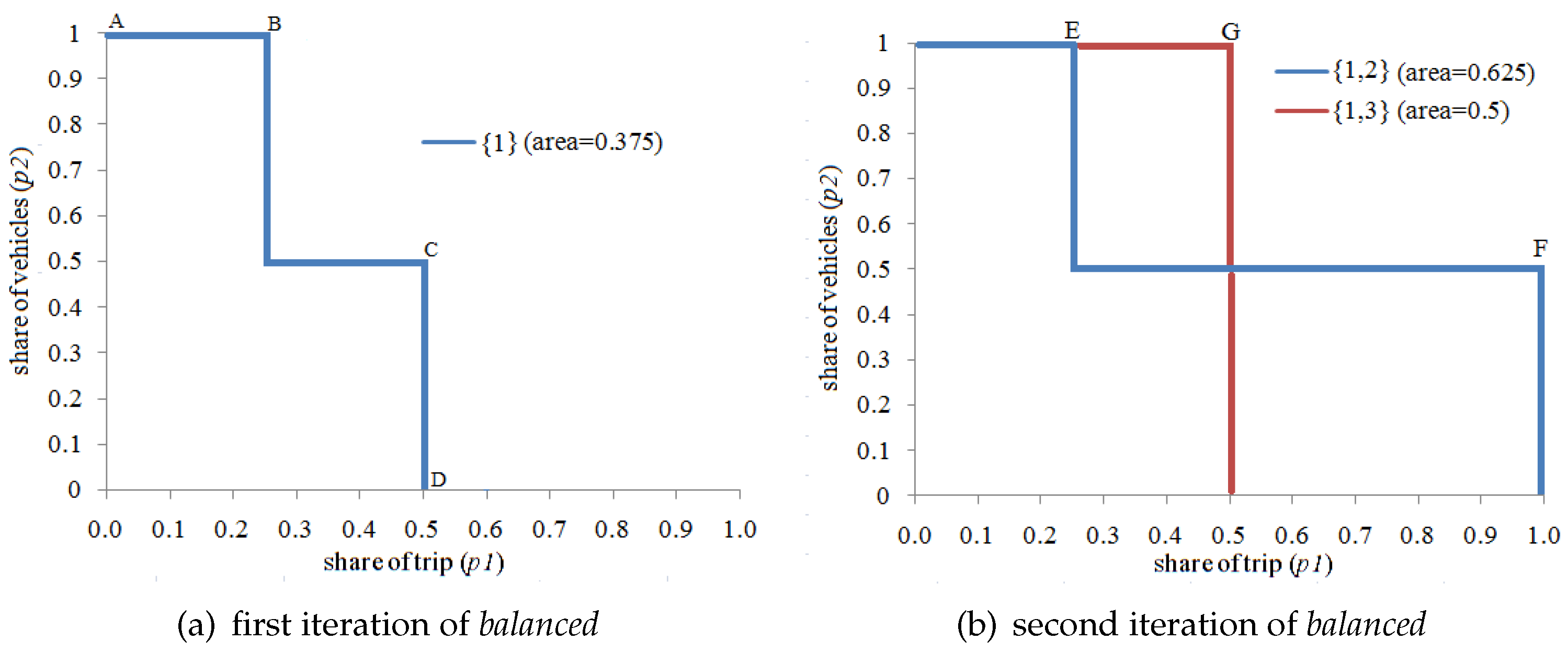
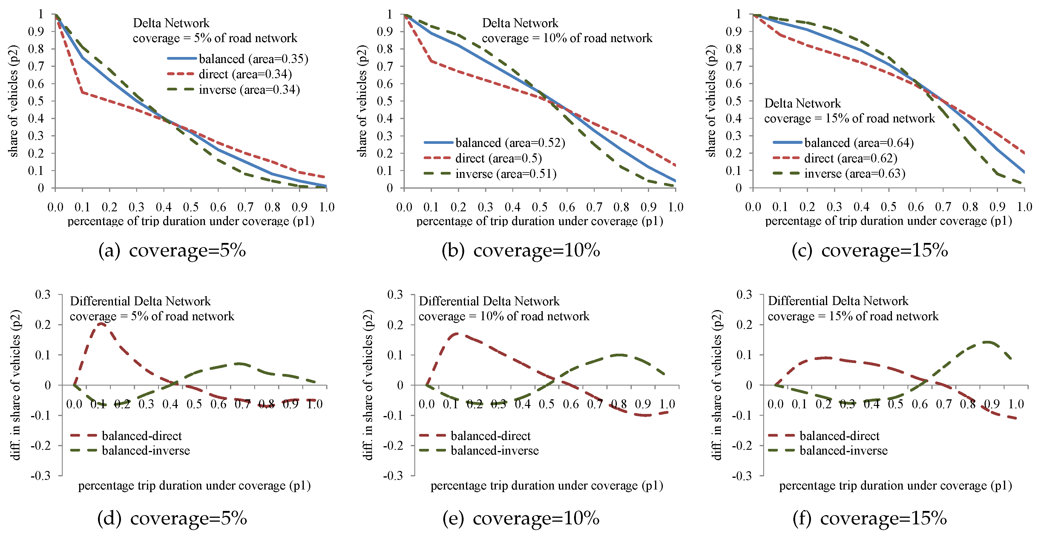
5.1. Strategy balanced: Uniform Distribution of Weights, Regardless of the Percentage Trip Duration under Coverage: An Alternative to Maximize the Area under the Delta Curve

By using an uniform distribution of weights across the entire range of “trip duration under coverage” (${\rho }_1$), we intend to maximize the area under the Delta curve. The area is computed using the trapezoidal rule [55], a technique for approximating the definite integral. Computing the integral demands partitioning the integration interval, applying the trapezoidal rule to each sub-interval, and summing the results. The approximation becomes more accurate as the resolution of the partition increases. In this work, we consider 1000 partitions dividing the x-axis (that has range [0…1]). In order to be more didactic, now we present an illustrative example: Let us suppose that we have only two vehicles traveling along the road network divided into 5 cells. Let us also assume that such vehicles remain the same amount of time inside each cell, and we have communication devices for covering only two cells ($\alpha$ = 2). Vehicle $v_1$ crosses cells {1,2}, while vehicle $v_2$ crosses cells {1,3,4,5}.

$$v_1=\{1,2\};$$

$$v_2=\{1,3,4,5\};$$

Since cell 1 is crossed by both vehicles, it intuitively maximizes the area under the Delta curve. After covering cell 1, we have vehicle $v_1$ covered during 50% of the trip, and vehicle $v_2$ covered during 25% of the trip. Figure 5a plots the Delta Network for this hypothetical scenario. Point A is (${\rho }_1$ = 0.00, ${\rho }_2$ = 1.00), i.e., 100% of vehicles are covered during 0% of the trip duration (true, vehicles $v_1$ and $v_2$). Point B is (${\rho }_1$ = 0.25, ${\rho }_2$ = 1.00), i.e., 100% of vehicles are covered during 25% of the trip duration (true, vehicles $v_1$ and $v_2$). Point C is (${\rho }_1$ = 0.50, ${\rho }_2$ = 0.50), i.e., 50% of vehicles are covered during 50% of the trip duration (true, vehicle $v_1$). Point D is (${\rho }_1$ = 0.50, ${\rho }_2$ = 0.00), i.e., no vehicle is covered more than 50% of the trip duration. Moreover, the plot indicates that covering cell 1 leads to area = 0.375.

In the second iteration, there are two possibilities: (a) Cover cell 2 crossed by vehicle $v_1$; (b) cover one of the cells crossed by vehicle $v_2$ (cell 3, cell 4, or, cell 5). In case the strategy selects one of the cells crossed by vehicle $v_2$ (let us say, cell 3), we notice vehicles $v_1$ and $v_2$ covered during 50% of the trip duration represented by point G in Figure 5b (red). In case the strategy covers cell 2, we notice vehicle $v_1$ covered during 100% of the trip duration, and vehicle $v_2$ covered during 25% of the trip duration. Thus, 100% of vehicles are covered during 25% of the trip duration (point E), and 50% of vehicles are covered during 100% of the trip duration (point F). Finally, the plot indicates that covering cells {1,2} leads to area = 0.625, while covering cells {1,3} leads to area = 0.500. Since the balanced strategy focuses on maximizing the area, the strategy selects cell 2 for coverage.

Figure 6 presents the performance of dl versus balanced for scenarios where {5%, 10%, 15%} of the road network is covered. Each plot presents the percentage of trip duration under coverage (y-axis) versus the share of vehicles receiving such coverage (x-axis). In fact, such measure is the Delta Network, showing how connectivity is distributed across the range of vehicles. The balanced strategy (blue) provides more coverage than the dl strategy (red). As we increase the number of covered cells (from 5% up to 15%), we notice an increase in the area below both curves. The maximum area below the curves is 1 (square with both sides equal 1). The legend of each plot indicates the area achieved. When considering Figure 6a, balanced reaches area = 0.35, while dl reaches area = 0.27. Deploying roadside units in 100% of the road network allows 100% of vehicles meeting coverage during 100% of the trip duration, yielding area = 1. Figure 6d–f present the Differential Delta Network, i.e., they plot only the difference “balanced minus dl”. As we can notice, all three plots are positive, also indicating that balanced provides better coverage than dl.

Figure 7 presents the layout of roadside units deployed by both strategies. Figure 7a shows the Cologne traffic. The darker is the area, the more intense is the flow. Figure 7b–e show the layout of roadside units deployed by dl for covering 5%, 10%, and 15% (respectively) of the road network. Similarly, Figure 7f–i present the layout of roadside units deployed by balanced for covering the same scenarios. When comparing the pairs of layouts considering the same scenario, we notice that dl and balanced follow a very distinct strategy. Since dl follows popular locations, most roadside units are deployed lined up, following the flow of vehicles. On the other hand, balanced follows a pattern based on circles emerging from the epicenter of traffic.

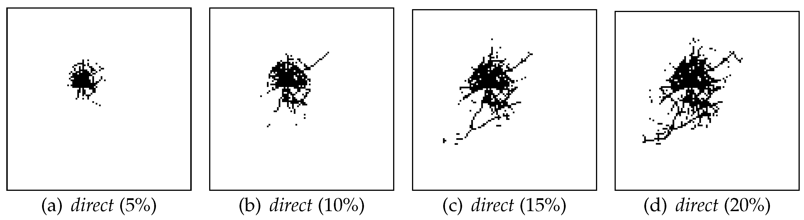
5.2. Strategy direct: Distribution of Weights Directly Proportional to the Percentage of Trip Traveled under Coverage: An Alternative to Prioritize Vehicles with High Coverage

Strategy direct considers a different score computation. Instead of assigning the same weight for all classes of coverage (as done by the strategy balanced), direct assumes weights equal to the value to the percentage of trip duration under coverage (weight = ${\rho }_1$), as presented in Figure 4b. By doing so, the strategy increases the reward for covering highly connected vehicles (instead of maximizing the area under the Delta curve).

Figure 8 shows the comparison between dl and direct. In Figure 8a–c, we notice that direct reduces the coverage for low connected vehicles, increasing the coverage for highly connected ones, as indicated by marks H, I, and J in such figures. We notice a distinct shape of coverage, different than the one presented by strategy balanced in the previous section. Such distinct shape of coverage is highlighted in Figure 8d–f, where the first half of the green area is negative (indicating the reduction of coverage for low connected vehicles), and the second half is highly positive (indicating increase of coverage of highly connected vehicles). Such shape of coverage is interesting when the applications running on top of the vehicular network demand highly connected vehicles (such as streaming delivery).

Figure 9a–d show the layout of roadside units provided by direct. Just like the strategy balanced, the strategy direct also deploy roadside units in circles from the epicenter of traffic. However, the layout provided by direct is much more concentrated around the epicenter of traffic (assuring more connectivity to highly connected vehicles). The pattern is characterized by connected islands of coverage along the core of the road network, an interesting topology when we intend high connectivy of vehicles in special zones, such as commercial zones in the city.

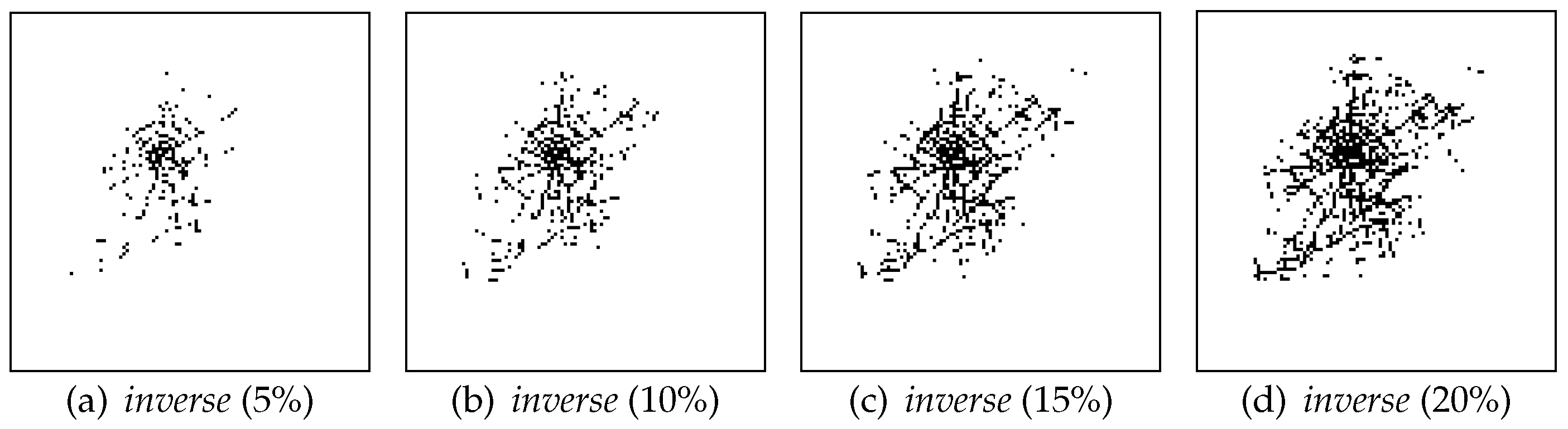
5.3. Strategy inverse: Distribution of Weights Inversely Proportional to the Percentage of Trip Traveled under Coverage: An Alternative to Prioritize Vehicles with Low Coverage

Strategy inverse assumes weights inversely proportional to the “trip duration under coverage” (i.e., weight = $1-{\rho }_1$), as presented in Figure 4c. It increases the reward for covering low connected vehicles, an interesting strategy when we intend to provide small contact opportunities for a large share of vehicles.

Figure 10 characterizes the strategy inverse using dl as baseline. We notice that inverse provides more connectivity than dl for all three scenarios presented in Figure 10a–c. When considering the shape of coverage, Figure 10d,e show better coverage when compared to other strategies in the first half of the x-axis (indicating that inverse is prioritizing the coverage of vehicles with small connectivity along the trip), while Figure 10e,f show the green curve negative for ${\rho }_1>0.80$, showing reduction in terms of highly connected vehicles.

Figure 11a–d Show the layout of roadside units provided by inverse. Just like the strategy balanced and direct, the strategy inverse also deploys roadside units in circles from the epicenter of traffic. However, the layout provided by the strategy inverse is much less concentrated around the epicenter of traffic. Such issue illustrates that the strategy inverse is more focused on providing coverage for new vehicles, than extending the coverage of highly connected ones.

In order to highlight differences among the proposed strategies (balanced, direct, inverse), we plot them all together. Figure 12a–c plot the Delta Network for the strategies balanced (blue), direct (red), and inverse (green). We consider the same coverage scenarios ranging from 5% up to 15% of the road network. We notice that strategy inverse (green) provides more connectivity than balanced (blue) in the first half of the x-axis. This indicates that inverse provides more low connected vehicles contacting roadside units. On the other hand, direct (red) provides more connectivity along the second half of the x-axis, indicating that direct increases the coverage of highly connected vehicles, while strategy balanced represents a trade-off between both strategies. By observing the legend of these figures, we also notice that balanced provides the largest area under the Delta curve.

Figure 12d–f present the Differential Delta Network of (i) direct compared to balanced, and (ii) inverse compared to balanced. The red curve indicates the value “balanced minus direct”, while the green curve plots “balanced minus inverse”. All three figures show the same behavior:

(a)

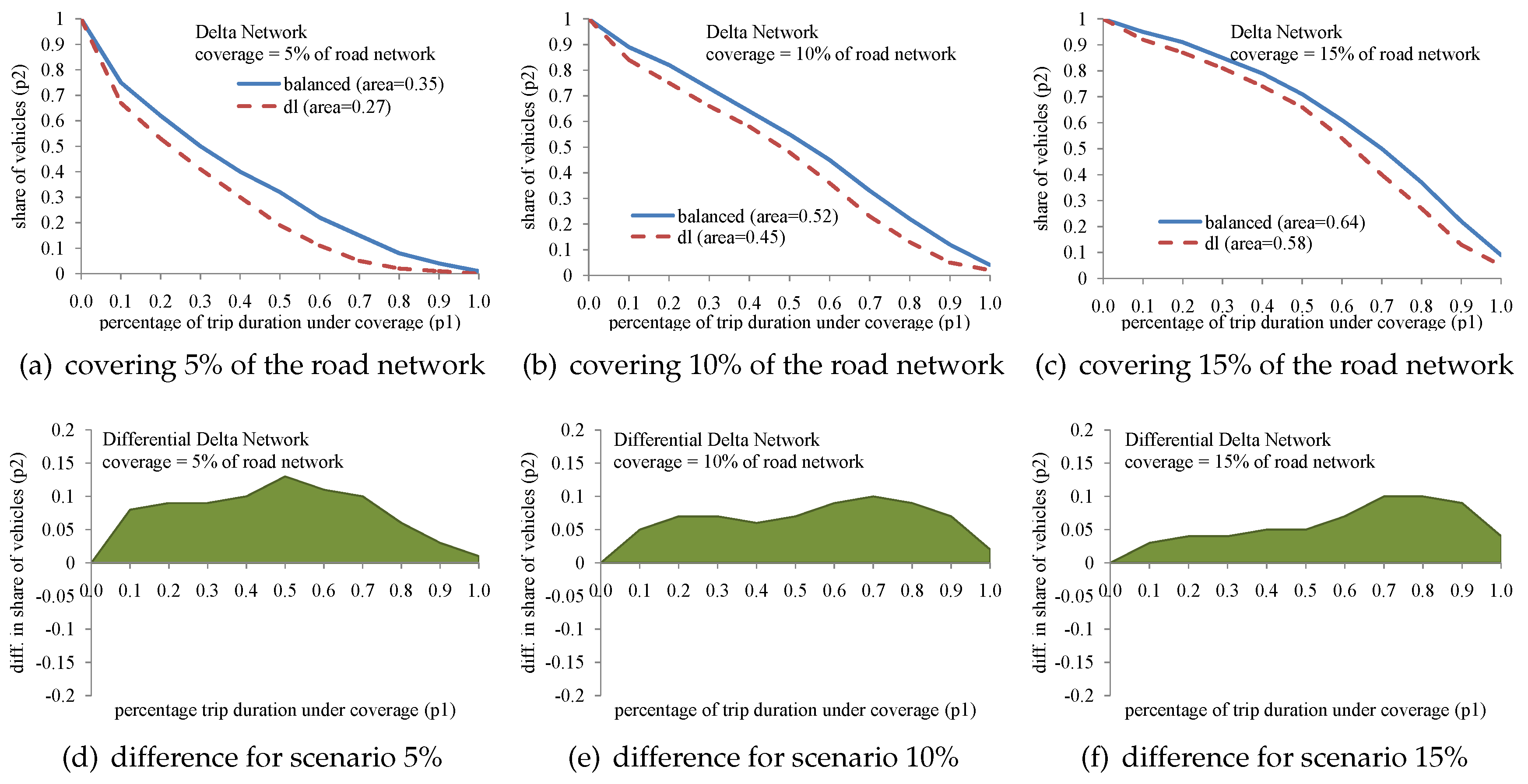
red curve (direct) positive in the first half of the x-axis indicates that balanced provides more connectivity than direct for low connected vehicles;

(b)

red curve (direct) negative in the second half of the x-axis indicates that balanced provides less connectivity than direct for highly connected vehicles;

(c)

green curve (inverse) negative in the first half of the x-axis indicates that balanced provides less connectivity than inverse for low connected vehicles;

(d)

green curve positive in the first half of the x-axis indicates that balanced provides more connectivity than inverse for highly connected vehicles.

Finally,

Table 1. Summary of strategies.

Strategy	Score Computation	Style of Coverage
balanced	select cell maximizing the area under the Delta curve	moderate density around the epicenter of traffic
direct	select cell prioritizing vehicles with high coverage	high density around the epicenter of traffic
inverse	select cell prioritizing vehicles with low/no coverage	low density around the epicenter of traffic

summarizes the most important characteristics of each strategy.

6. Conclusions

In this work, we discuss the performance of vehicular networks in terms of the metric Delta Network [29]. The Delta Network characterizes the connectivity of the vehicular network through the percentage of travel time in which vehicles are connected to roadside units. In summary, this article reviews the concept of the Delta Network and extends its study through the presentation of a general heuristic in Algorithm 1, which is based on the definition of scores to identify areas of the road network that should receive coverage under different objectives. We consider the Vehicular Mobility Trace of Cologne, Germany, with the road network partitioned into a grid-like structure of dimensions 100 × 100, resulting in urban cells of dimension 270 m × 260 m, holding more than 75 thousand vehicles.

After defining the general heuristic, we show how small changes in the score computation can generate very distinct (and interesting) patterns of coverage, each one suited to a given coverage objective. The definition of the score is based on the number of vehicles meeting coverage in relation to the distance traveled. In particular, when we consider the same weight for all travel classes (strategy balanced), we obtain as a result the maximization of the area under the Delta curve. On the other hand, when we consider the score directly proportional to the percentage of the trip that vehicles travel with coverage (strategy direct), we obtain a pattern that privileges the coverage of vehicles with high connectivity, resulting in increasing the share of vehicles experiencing high coverage, where the resulting layout of roadside units becomes more condensed around the traffic epicenter.

However, when we consider scores inversely proportional to the percentage of the trip that vehicles meet coverage, we get a more inclusive pattern where new vehicles get the opportunity to meet coverage. In such a case, we have the least concentrated roadside units layout when considering all experiments performed along this study (strategy inverse). Finally, for all strategies evaluated, the layout of roadside units follows a circular pattern around the traffic epicenter.

References

1. Washburn, D.; Sindhu, U.; Balaouras, S.; Dines, R.A.; Hayes, N.; Nelson, L.E. Helping CIOs understand “smart city” initiatives. Growth 2009, 17, 1–17. [Google Scholar]
2. Nam, T.; Pardo, T.A. Conceptualizing smart city with dimensions of technology, people, and institutions. In Proceedings of the 12th Annual International Digital Government Research Conference: Digital Government Innovation in Challenging Times, College Park, MD, USA, 12–15 June 2011; pp. 282–291. [Google Scholar]
3. Caragliu, A.; Del Bo, C.; Nijkamp, P. Smart cities in Europe. J. Urban Technol. 2011, 18, 65–82. [Google Scholar] [CrossRef]
4. Van Audenhove, F.J.; Korniichuk, O.; Dauby, L.; Pourbaix, J. The Future of Urban Mobility 2.0: Imperatives to Shape Extended Mobility Ecosystems of Tomorrow; Arthur D. Little in collaboration with UITP: Brussels, Belgium, 2014. [Google Scholar]
5. Lozano-Perez, T. Autonomous Robot Vehicles; Springer Science & Business Media: Berlin, Germany, 2012. [Google Scholar]
6. Katzev, R. Car sharing: A new approach to urban transportation problems. Anal. Soc. Issues Public Policy 2003, 3, 65–86. [Google Scholar] [CrossRef]
7. Silva, C.M.; Masini, B.M.; Ferrari, G.; Thibault, I. A Survey on Infrastructure-Based Vehicular Networks. Mobile Inf. Syst. 2017, 2017, 28–56. [Google Scholar]
8. Dighriri, M.; Lee, G.M.; Baker, T. Measurement and Classification of Smart Systems Data Traffic Over 5G Mobile Networks. In Technology for Smart Futures; Dastbaz, M., Arabnia, H., Akhgar, B., Eds.; Springer International Publishing: Cham, Switzerland, 2018; pp. 195–217. [Google Scholar]
9. Swain, P.; Christophorou, C.; Bhattacharjee, U.; Silva, C.M.; Pitsillides, A. Selection of UE-based Virtual Small Cell Base Stations using Affinity Propagation Clustering. In Proceedings of the 2018 14th InternationalWireless Communications Mobile Computing Conference (IWCMC), Limassol, Cyprus, 25–29 June 2018; pp. 1104–1109. [Google Scholar]
10. Vegni, A.M.; Loscri, V. A survey on vehicular social networks. IEEE Commun. Surv. Tutor. 2015, 17, 2397–2419. [Google Scholar] [CrossRef]
11. Silva, C.M.; Sarubbi, J.F.; Silva, D.F.; Porto, M.F.; Nunes, N.T. A Mixed Load Solution for the Rural School Bus Routing Problem. In Proceedings of the 2015 IEEE 18th International Conference on Intelligent Transportation Systems (ITSC), Las Palmas, Spain, 15–18 September 2015; pp. 1940–1945. [Google Scholar]
12. Lee, S.; Tewolde, G.; Kwon, J. Design and implementation of vehicle tracking system using GPS/GSM/GPRS technology and smartphone application. In Proceedings of the 2014 IEEE World Forum on Internet of Things (WF-IoT), Seoul, Korea, 6–8 March 2014; pp. 353–358. [Google Scholar]
13. Araujo, R.; Igreja, A.; de Castro, R.; Araujo, R. Driving coach: A smartphone application to evaluate driving efficient patterns. In Proceedings of the 2012 IEEE Intelligent Vehicles Symposium (IV), Alcala de Henares, Spain, 3–7 June 2012; pp. 1005–1010. [Google Scholar]
14. Johnson, D.A.; Trivedi, M.M. Driving style recognition using a smartphone as a sensor platform. In Proceedings of the 2011 14th International IEEE Conference on Intelligent Transportation Systems (ITSC), Washington, DC, USA, 5–7 October 2011; pp. 1609–1615. [Google Scholar]
15. Eriksson, J.; Girod, L.; Hull, B.; Newton, R.; Madden, S.; Balakrishnan, H. The pothole patrol: using a mobile sensor network for road surface monitoring. In Proceedings of the ACM MobiSys, Breckenridge, CO, USA, 17–20 June 2008. [Google Scholar]
16. McClellan, S.; Follmer, T.; Maynard, E.; Capps, E.; Larson, G.; Ord, D.; Eyre, R.; Russon, V.; Watkins, C.; Vo, V.; et al. System and Method for Monitoring Vehicle Parameters and Driver Behavior. U.S. Patent 8,630,768, 2014. [Google Scholar]
17. Oliveira, T.R.; Silva, C.M.; Macedo, D.F.; Nogueira, J.M. SNVC: Social networks for vehicular certification. Comput. Netw. 2016, 111, 129–140. [Google Scholar] [CrossRef]
18. Zhang, Z.; Boukerche, A.; Ramadan, H. Design of a lightweight authentication scheme for IEEE 802.11p vehicular networks. Ad Hoc Netw. 2012, 10, 243–252. [Google Scholar] [CrossRef]
19. Koukoumidis, E.; Peh, L.S.; Martonosi, M.R. SignalGuru: leveraging mobile phones for collaborative traffic signal schedule advisory. In Proceedings of the 9th International Conference on Mobile Systems, Applications, and Services, Bethesda, MD, USA, 28 June–1 July 2011; pp. 127–140. [Google Scholar]
20. Rybick, J.; Scheuermann, B.; Kiess, W.; Lochert, C.; Fallahi, P.; Mauve, M. Challenge: Peers on wheels—A road to new traffic information systems. In Proceedings of the 13th Annual ACM International Conference on Mobile Computing and Networking (MobiCom 2007), Montreal, QC, Canada, 9–14 September 2007; pp. 215–221. [Google Scholar]
21. Zaldivar, J.; Calafate, C.T.; Cano, J.C.; Manzoni, P. Providing accident detection in vehicular networks through OBD-II devices and android-based smartphones. In Proceedings of the 2011 IEEE 36th Conference on Local Computer Networks (LCN), Bonn, Germany, 4–7 October 2011; pp. 813–819. [Google Scholar]
22. Thompson, C.; White, J.; Dougherty, B.; Albright, A.; Schmidt, D.C. Using smartphones to detect car accidents and provide situational awareness to emergency responders. In Mobile Wireless Middleware, Operating Systems, and Applications; Springer: Berlin, Germany, 2010; pp. 29–42. [Google Scholar]
23. Masini, B.; Bazzi, A.; Zanella, A. A survey on the roadmap to mandate on board connectivity and enable V2V-based vehicular sensor networks. Sensors 2018, 18, 2207. [Google Scholar] [CrossRef]
24. Mukhtar, A.; Xia, L.; Tang, T.B. Vehicle Detection Techniques for Collision Avoidance Systems: A Review. IEEE Trans. Intell. Transp. Syst. 2015, 16, 2318–2338. [Google Scholar] [CrossRef]
25. Di Bernardo, M.; Salvi, A.; Santini, S. Distributed consensus strategy for platooning of vehicles in the presence of time-varying heterogeneous communication delays. IEEE Trans. Intell. Transp. Syst. 2015, 16, 102–112. [Google Scholar] [CrossRef]
26. Silva, C.M.; Aquino, A.L.L.; Meira, W., Jr. Smart Traffic Light for Low Traffic Conditions. Mob. Netw. Appl. 2015, 1–9. [Google Scholar] [CrossRef]
27. Ferreira, M.C.P.; Tonguz, O.; Fernandes, R.J.; DaConceicao, H.M.F.; Viriyasitavat, W. Methods and Systems for Coordinating Vehicular Traffic Using in-Vehicle Virtual Traffic Control SignalS Enabled by Vehicle-to-Vehicle Communications. U.S. Patent 8,972,159, 2015. [Google Scholar]
28. Kim, I.H.; Bong, J.H.; Park, J.; Park, S. Prediction of driver’s intention of lane change by augmenting sensor information using machine learning techniques. Sensors 2017, 17, 1350. [Google Scholar] [CrossRef] [PubMed]
29. Silva, C.M.; Meira, W., Jr. Evaluating the Performance of Heterogeneous Vehicular Networks. In Proceedings of the 2015 IEEE 82nd Vehicular Technology Conference (VTC2015-Fall), Boston, MA, USA, 6–9 September 2015; pp. 1–5. [Google Scholar]
30. Weeratunga, K.; Somers, A. Connected Vehicles: Are We Ready? Internal Report on Potential Implications for Main RoadsWA; Main RoadsWestern Australia: Perth, Australia, 2015. [Google Scholar]
31. Lu, N.; Cheng, N.; Zhang, N.; Shen, X.; Mark, J.W. Connected vehicles: Solutions and challenges. IEEE Internet Things J. 2014, 1, 289–299. [Google Scholar] [CrossRef]
32. Sanguesa, J.A.; Fogue, M.; Garrido, P.; Martinez, F.J.; Cano, J.C.; Calafate, C.T. A Survey and Comparative Study of Broadcast Warning Message Dissemination Schemes for VANETs. Mobile Inf. Syst. 2016, 2016, e16. [Google Scholar] [CrossRef]
33. Liu, K.; Lee, V.S. RSU-based real-time data access in dynamic vehicular networks. In Proceedings of the 2010 13th International IEEE Conference on Intelligent Transportation Systems (ITSC), Funchal, Portugal, 19–22 September 2010; pp. 1051–1056. [Google Scholar]
34. Bruno, R.; Nurchis, M. Robust and efficient data collection schemes for vehicular multimedia sensor Networks. In Proceedings of the 2013 IEEE 14th International Symposium and Workshops on World of Wireless, Mobile and Multimedia Networks (WoWMoM), Madrid, Spain, 4–7 June 2013; pp. 1–10. [Google Scholar]
35. Shumao, O.; Kun, Y.; Hsiao-Hwa, C.; Alex, G. A selective downlink scheduling algorithm to enhance quality of VOD services for WAVE networks. EURASIP J. Wirel. Commun. Netw. 2009, 2009, 2. [Google Scholar]
36. Zhang, Y.; Zhao, J.; Cao, G. Service Scheduling of Vehicle-Roadside Data Access. Mob. Netw. Appl. 2010, 15, 83–96. [Google Scholar] [CrossRef]
37. Dighriri, M.; Lee, G.M.; Baker, T. Applying Scheduling Mechanisms Over 5G Cellular Network Packets Traffic. In Third International Congress on Information and Communication Technology; Yang, X.S., Sherratt, S., Dey, N., Joshi, A., Eds.; Springer: Singapore, 2019; pp. 119–131. [Google Scholar]
38. Baker, T.; García-Campos, J.M.; Reina, D.G.; Toral, S.; Tawfik, H.; Al-Jumeily, D.; Hussain, A. GreeAODV: An Energy Efficient Routing Protocol for Vehicular Ad Hoc Networks. In Intelligent Computing Methodologies; Huang, D.S., Gromiha, M.M., Han, K., Hussain, A., Eds.; Springer International Publishing: Cham, Switzerland, 2018; pp. 670–681. [Google Scholar]
39. Korkmaz, G.; Ekici, E.; Ozguner, F. A cross-layer multihop data delivery protocol with fairness guarantees for vehicular networks. IEEE Trans. Veh. Technol. 2006, 55, 865–875. [Google Scholar] [CrossRef]
40. Hadaller, D.; Keshav, S.; Brecht, T. MV-MAX: Improving wireless infrastructure access for multi-vehicular communication. In Proceeding of the 2006 SIGCOMM Workshop, Pisa, Italy, 11–15 September 2006; pp. 269–276. [Google Scholar]
41. Bazzi, A.; Masini, B.M.; Zanella, A.; Pasolini, G. IEEE 802.11P for Cellular Offloading in Vehicular Sensor Networks. Comput. Commun. 2015, 60, 97–108. [Google Scholar] [CrossRef]
42. Trullols-Cruces, O.; Fiore, M.; Barcelo-Ordinas, J. Cooperative download in vehicular environments. IEEE Trans. Mob. Comput. 2012, 11, 663–678. [Google Scholar] [CrossRef]
43. Silva, C.M.; Silva, F.A.; Sarubbi, J.F.; Oliveira, T.R.; Meira, W., Jr.; Nogueira, J.M.S. Designing mobile content delivery networks for the Internet of vehicles. Veh. Commun. 2017, 8, 45–55. [Google Scholar] [CrossRef]
44. Lochert, C.; Scheuermann, B.; Wewetzer, C.; Luebke, A.; Mauve, M. Data Aggregation and Roadside Unit Placement for a Vanet Traffic Information System. In Proceedings of the Fifth ACM International Workshop on VehiculAr Inter-NETworking, San Francisco, CA, USA, 15 September 2008; pp. 58–65. [Google Scholar]
45. Cavalcante, E.S.; Aquino, A.L.; Pappa, G.L.; Loureiro, A.A. Roadside Unit Deployment for Information Dissemination in a VANET: An Evolutionary Approach. In Proceedings of the Fourteenth International Conference on Genetic and Evolutionary Computation Conference Companion, Philadelphia, PA, USA, 7–11 July 2012; pp. 27–34. [Google Scholar]
46. Aslam, B.; Amjad, F.; Zou, C. Optimal roadside units placement in urban areas for vehicular networks. In Proceedings of the 2012 IEEE Symposium on Computers and Communications (ISCC), Cappadocia, Turkey, 1–4 July 2012; pp. 000423–000429. [Google Scholar]
47. Liang, Y.; Liu, H.; Rajan, D. Optimal Placement and Configuration of Roadside Units in Vehicular Networks. In Proceedings of the 2012 IEEE 75th Vehicular Technology Conference (VTC Spring), Yokohama, Japan, 6–9 May 2012; pp. 1–6. [Google Scholar]
48. Trullols, O.; Fiore, M.; Casetti, C.; Chiasserini, C.; Ordinas, J.B. Planning roadside infrastructure for information dissemination in intelligent transportation systems. Computer Commun. 2010, 33, 432–442. [Google Scholar] [CrossRef]
49. Silva, C.M.; Meira, W.; Sarubbi, J.F.M. Non-Intrusive Planning the Roadside Infrastructure for Vehicular Networks. IEEE Trans. Intell. Transp. Syst. 2016, 17, 938–947. [Google Scholar] [CrossRef]
50. Bazzi, A.; Masini, B.M.; Andrisano, O. On the Frequent Acquisition of Small Data Through RACH in UMTS for ITS Applications. IEEE Trans. Veh. Technol. 2011, 60, 2914–2926. [Google Scholar] [CrossRef]
51. Zheng, Z.; Sinha, P.; Kumar, S. Alpha Coverage: Bounding the Interconnection Gap for Vehicular Internet Access. In Proceedings of the INFOCOM 2009, Rio de Janeiro, Brazil, 19–25 April 2009; pp. 2831–2835. [Google Scholar]
52. Sarubbi, J.F.M.; Silva, C.M. Delta-r: A novel and more economic strategy for allocating the roadside infrastructure in vehicular networks with guaranteed levels of performance. In Proceedings of the NOMS 2016 IEEE/IFIP Network Operations and Management Symposium, Istanbul, Turkey, 25–29 April 2016; pp. 665–671. [Google Scholar]
53. Silva, C.M.; Silva, F.; Nogueira, J.M.S. Delivering Heterogeneous Contents with Distinct Performance Requirements in Vehicular Networks. In Proceedings of the 2016 IEEE Symposium on Computers and Communications (ISCC), Messina, Italy, 27–30 June 2016. [Google Scholar]
54. Uppoor, S.; Trullols-Cruces, O.; Fiore, M.; Barcelo-Ordinas, J.M. Generation and analysis of a large-scale urban vehicular mobility dataset. IEEE Trans. Mob. Comput. 2014, 13, 1061–1075. [Google Scholar] [CrossRef]
55. Rice, S. Efficient evaluation of integrals of analytic functions by the trapezoidal rule. Bell Syst. Tech. J. 1973, 52, 707–722. [Google Scholar] [CrossRef]
Figure 1. Delta governs the combinations of ρ 1 (share of trip under coverage) and ρ 2 (share of vehicles meeting coverage). Source: Silva et al. [29].
Futureinternet 11 00001 g001
Figure 2. Partitioning the road network in a grid-like structure. Source: [29] With kindly permission.
Futureinternet 11 00001 g002
Figure 3. Percentage of road network that must be covered in order to achieve the Delta Network for pairs of ρ 1 and ρ 2 when solving the deployment using Delta-g. Recall that ρ 2 indicates the share of vehicles that must be connected during ρ 1 percent of the trip duration. Results consider the Cologne mobility trace. Source: Silva et al. [53] with kindly permission.
Futureinternet 11 00001 g003
Figure 4. Figure shows the distribution of weights used for computing the score indicating the next cell to be covered by Algorithm 1. (a) Shows the distribution used for the strategy balanced. All ranges of “percentage trip duration under coverage” receive the same weight, and the goal is to maximize the area under the Delta curve. (b) Shows the distribution used for the strategy direct, where weights are directly proportional to the “percentage trip duration under coverage” shown in the x-axis. By using such distribution, we intend to increase the share of highly connected vehicles. (c) Shows the distribution used for the strategy inverse, where weights are inversely proportional to the “percentage trip duration under coverage”. By using such distribution, we intend to democratize the coverage.
Futureinternet 11 00001 g004
Figure 5. Didactic example on how the balanced strategy operates. (a) Presents the Delta Network after covering cell 1. (b) Presents the Delta Network considering two options: (a) Covering cell 2; (b) covering cell 3. Since covering cell 2 leads to a major area under the curve, cell 2 is selected.
Futureinternet 11 00001 g005
Figure 6. Delta Network: dl deploys roadside units at the most popular locations (red color), while balanced assumes an uniform distribution of weights (color blue). The y-axis indicates the share of vehicles ( ρ 2 ), while the x-axis indicates percentage of trip under coverage ( ρ 1 ). (ac) Consider coverage ranging from 5% up to 15% of the road network. (df) Represent the difference “balanced minus dl”. Since the green area is positive, balanced is always providing more coverage.
Futureinternet 11 00001 g006
Figure 7. Layout of roadside units deployed by dl and balanced. (a) Shows the Cologne traffic. The darker the area, the more intense is the flow. (be) Show the layout of roadside units deployed by dl for covering 5%, 10%, 15%, and 20% (respectively) of the road network. Similarly, (fi) present the layout of roadside units deployed by balanced for covering the same scenarios.
Futureinternet 11 00001 g007
Figure 8. Strategy dl deploys roadside units at the most popular locations (red color), while direct assumes a distribution of weights equal to ρ 1 (color blue). The y-axis indicates the share of vehicles ( ρ 2 ), while the x-axis indicates percentage of trip under coverage ( ρ 1 ). (ac) Consider coverage ranging from 5% up to 15% of the road network. (df) Represent the difference “direct minus dl”.
Futureinternet 11 00001 g008
Figure 9. (ad) Show the layout of roadside units deployed by direct for covering 5%, 10%, 15%, and 20% (respectively) of the road network. We notice that direct presents a denser distribution of roadside units around the epicenter of traffic when compared to strategy balanced (Figure 7f–i).
Futureinternet 11 00001 g009
Figure 10. Strategy dl deploys roadside units at the most popular locations (red color), while inverse assumes a distribution of weights inversely proportional to ρ 1 (color blue). The y-axis indicates the share of vehicles ( ρ 2 ), while the x-axis indicates percentage of trip under coverage ( ρ 1 ). (ac) Consider coverage ranging from 5% up to 15% of the road network. (df) Represent “inverse minus dl”.
Futureinternet 11 00001 g010
Figure 11. (ad) Show the layout of roadside units deployed by inverse for covering 5%, 10%, 15%, and 20% (respectively) of the road network. When compared to balanced and direct, we notice that inverse presents the lowest density of roadside units around the epicenter of traffic.
Futureinternet 11 00001 g011
Figure 12. (ac) Present the Delta Network in a single plot for the three proposed strategies: balanced (blue), direct (red), and inverse (green). (df) Present the Differential Delta Network. In these figures, the red curve indicates the value “balanced minus direct”, while the green curve shows “balanced minus inverse”.
Futureinternet 11 00001 g012