A Scheme to Design Community Detection Algorithms in Various Networks

Abstract

Network structures, consisting of nodes and edges, have applications in almost all subjects. A set of nodes is called a community if the nodes have strong interrelations. Industries (including cell phone carriers and online social media companies) need community structures to allocate network resources and provide proper and accurate services. However, most detection algorithms are derived independently, which is arduous and even unnecessary. Although recent research shows that a general detection method that serves all purposes does not exist, we believe that there is some general procedure of deriving detection algorithms. In this paper, we represent such a general scheme. We mainly focus on two types of networks: transmission networks and similarity networks. We reduce them to a unified graph model, based on which we propose a method to define and detect community structures. Finally, we also give a demonstration to show how our design scheme works.

1. Introduction

Our real world consists of elements associated with relations. The group, consisting of elements with relationships among them, is called a network. Real-world networks are mostly not random as they reveal big homogeneity, a high level of order and organization [1]. For example, a person would have stronger relations with his colleagues working at the same place than those working at some other branches. The observation inspires people to partition the elements into groups (communities) such that the relations are strong and dense within the groups but sparse and weak among them [1,2,3].

Community detections have widespread applications. Amazon groups customers purchasing similar products together for better commodity recommendations. Facebook clusters its users by relationships and hobbies for accurate friend and circle suggestions. Carriers group the locations among which customers have high transportation demands for better transportation resource allocation.

Due to the omnipresent community structures in practice, researchers try to find proper algorithms to detect them. There are mainly four traditional methods [1]: graph partitioning [4], hierarchical clustering [5], partitional clustering [6,7], and spectral clustering [8,9,10,11]. These methods are designed for different purposes and reveal many fundamental network properties. After that, many related algorithms are proposed (for instances, modularity-based methods [12,13,14], dynamic algorithms [15], methods based on statistical inference [16,17], maximum likelihood [18,19] and network motifs [20,21,22]). In addition, some detection algorithms’ clustering nodes according to their attribute similarities are also reported [23]. Recent research reveals the equivalence between the modularity optimization and maximum likelihood algorithms [24], and significant contributions have been made regarding the detection efficiency [25,26,27].

Most algorithms work well in the areas from which they are derived. However, the reliabilities outside their zones are controversial. Recent research has shown that a particular network can be derived from multiple backgrounds, which can have various ground truth results. In other words, for one graph, the detection results of an algorithm may be considered good under one background but bad under another one. This implies that there does not exist a general detection algorithm to solve all community detection problems [28].

Although it has been proved that no general detection method exists, we believe the existence of a design procedure for deriving ad hoc algorithms. In this paper, we propose such a general design scheme. In particular, we represent a method for converting practical problems into graph models. We mainly focus on the networks constructed by material transmission and node attribute similarities. Based on the graph models, we discuss the common properties shared by various community definitions, followed by a method for detecting them. Finally, we provide a demonstration to show how our scheme works. The comparison results show that an algorithm derived from our scheme can produce reasonable detection results.

We want to emphasize that our scheme does not provide a deterministic way to implement community detection. Instead, we discuss the common properties shared by the most of the algorithms. While our work can facilitate the development of new algorithms, readers need to derive algorithms according to their practical problems. Thus, our work does not conflict with but supplements the result reported in Ref. [28].

The rest of the paper is organized as follows. Section 2 provides a brief review of the popular community detection algorithms. Section 3 discusses the general properties of the graph models that should be considered during the model construction. Based on this, in Section 4, we define the community structures and discuss their fundamental properties. We also provide a corresponding detection algorithm. Finally, we derive an algorithm through our scheme for demonstration in Section 5. We also discuss its performance by comparing it with other famous algorithms.

2. Related Work

The research of community detection starts from solving practical problems. For instance, Kernighan–Lin algorithm [4] clusters digital components into similar size groups with the minimized inter-group connections. In this way, engineers decrease the electronic device costs and enhance their stability.

Conventionally, real-world networks are represented by nodes and edges. Two nodes connected by edges have some kind of relations. Although the meanings of relations vary in different problems, there are two main types: two nodes are related if

• There is material transmission between them, and/or
• they share some identical or similar properties.

The material here represents concrete objects (like goods) or information (like data packages). A typical example is the transportation among cities. The cities among which people can easily travel have stronger relations and could be considered as a community [29].

Node attribute similarities also derive relations. In protein–protein interaction networks, biologists cluster proteins with equivalent or similar functions into one group [30]. Here, the relations are their function similarities. In social networks, the people active in similar locations and/or the time slots could be considered as a community. Here, the relations are the location and schedule similarities.

Based on graph models, lots of community detection algorithms have been proposed.

Graph partitioning method groups the vertices into a predefined number of communities and minimize the number of edges among them. The algorithms belonging to this method can perfectly solve many practical problems. However, they cannot be adapted to community detections as the algorithms require a pre-specified number of groups that is generally unknown in a community detection problem [1]. In addition, the graph partitioning method is not derived from an explicit definition of communities. Thus, there is no guarantee that the method finds the vertex groups consistent with our intuitions.

Real-world networks commonly have hierarchical structures from which the abstracted graph models are usually inherited. The related detection algorithms fall into two categories: agglomerative (bottom–up) approach and divisive (top–down) approach [5]. Briefly, the agglomerative approach starts by considering each node as a community and merges the community pairs while moving up the hierarchy. The divisible algorithm works in the opposite way. It starts by grouping all the nodes in one cluster and performs splitting recursively as moving down the hierarchy.

Partitional clustering also plays an important role in the graph clustering family. In order to apply the algorithm, the user must specify the number of clusters. Thus, it has the same disadvantages as the ones belonging to graph partitioning [1]. The method puts all nodes in a metric space, and thus the distance between each pair of the nodes in the space is defined. The distance here can be considered as a measure of the dissimilarities between the nodes. The algorithm needs to cluster the nodes into a fixed number of groups to minimize a pre-specified cost function.

All community detection methods and techniques related to matrix eigenvectors belong to spectral clustering. The clustering method requires a distance function to measure the similarity among the objects. The fundamental idea of the algorithm is to use eigenvectors to cluster objects by connectedness rather than the distance. Although there are many successful applications in image segmentation and machine learning, researchers have already found several fundamental limitations. For instance, spectral clustering would fail if it uses the first k eigenvectors to find k clusters but confronts with clusters of various scales regarding a multi-scale landscape potential [31].

3. Concrete Problem Reduction

Intuitively, a community is some set of objects that have strong interrelations. In this section, we discuss how these relations are constructed and what properties can be shared by them. We focus on the relations derived in two ways: material transmission (Section 3.1) and node attribute similarities (Section 3.2). For both types, we first discuss the properties shared by the relations under various backgrounds. Then, we provide a scheme to abstract a concrete network into the node-edge model, which will be used for defining and detecting communities in Section 4. In Section 3.3, we discuss the relations between these two types of networks. We also show that they can be reduced to the same graph model.

3.1. Transmission Network

In this section, we discuss the relation derived from material transmission. The materials here can represent both material substance (like goods) or information (like data). Intuitively, the objects that can easily communicate with each other have strong relations. Then, these objects can somehow be considered as a community. We start our discussion by showing how a transmission network is constructed. Based on this, we derive the special relation strength measurement (SRSM) for measuring the relation of two nodes that have direct connections. Since SRSM cannot represent all the relations in a practical transmission network, we derived a generalized one called relation strength measurement for transmission network (RSMFTN). Finally, we prove that the shortest distance function is in fact an RSMFTN.

Our discussion is based on the following definitions and assumptions.

Assumption 1.

For any material, there is a minimal transmission unit, which is named point.

Definition 1 (Node).

The objects that receive and send point are nodes.

Definition 2 (Medium).

The one through which the points are propagated is a medium.

Nodes, media and points construct the transmission relations and determine their properties. We call a network based on the transmission relations transmission network. Two important characteristics in this network type are the number of points transferred and the time consumed in a transmission process. Their ratio is termed as speed.

Definition 3 (Speed).

Speed is the number of points transferred in a unit time interval.

The transmission capability can be described by the speed function of time (denoted by f). We first consider the node pairs connected by media directly. The behaviour of f depends on the properties of the nodes, media, and points. Thus, its algebraic expression cannot be given unless all the properties are designated. However, some properties should be shared by all transmission networks. Figure 1 represents how the speed function f changes for a pair of nodes $(u,v)$ connected by media directly. In particular, the speed function $f_{(u,v)}(t)$ has value zero when the transmission starts due to the latency of the point sending, propagation and reception.

We call the moment that the function value becomes nonzero the shortest transmission time (STT) (theoretically, $STT=\mathrm{sending}\mathrm{time}+\mathrm{transmission}\mathrm{time}+\mathrm{receiving}\mathrm{time}$). In addition, the speed function is upper bounded as the transmission speed cannot approach infinity in practice. We call the least upper bound theoretically transmission speed (TTS). Remarkably, TTS may never be reached and is thus not very useful. To solve the problem, we can choose some proper threshold $\delta \in {\mathbb{R}}^{*}$, the lowest acceptable speed. We call the time to reach the threshold the critical moment (CM).

Remark 1.

Suppose two towns A and B are connected by a river. A is upstream of B. For goods transported through the river, due to the water stream, the transformation speed from A to B is higher than the one in the opposite direction. Thus, $f_{(A,B)}(t)\ge f_{(B,A)}(t)$. This example implies that, in general, $f_{(u,v)}(t)\ne f_{(v,u)}(t)$.

The speed function characterizes the relation properties in a transmission network. Based on the function and the objectives needed to be achieved in a concrete problem, we can devise a measurement of the relation strength for a pair of nodes connected by the medium directly. We call this measurement special relation strength measurement (SRSM) which should have the following properties:

• The shorter STT is, the stronger the corresponding relation is.
• The shorter CM is, the stronger the corresponding relation is.
• The shorter the time to transfer a certain number of points is, the stronger the corresponding relation is.

Although a proper SRSM cannot be constructed until a concrete problem is given, several key properties should be shared by all SRSMs. In particular, relations of a transmission network should not cancel each other out. Thus, the SRSM is non-negative. In addition, the self-related relation is the strongest as the transmission speed is unbounded. Intuitively, all SRSMs should have the same value in this case and so are assigned value zero. In addition, the relation strength will get weaker if the function value increases. To sum up, we have

Definition 4 (Special relation strength measurement (SRSM)).

For a network, let s be a real-valued function defined on the set of node pairs that are directly connected by media. Then, s is an SRSM if

1. 

$s(u,v)\ge 0$, and

2. 

$s(u,v)=0$ if and only if $u=v$.

Remark 2.

By Remark 1, for a pair of nodes $(u,v)$, $f_{(u,v)}(t)\ne f_{(v,u)}(t)$ in general. Thus, for SRSMs, we also have $s(u,v)\ne s(v,u)$.

By SRSM, the transmission network is reduced to a graph model. Specifically, the nodes are represented by the vertices. Two nodes directly connected by the medium are linked by an edge of the weight given by the SRSM. In general, the graph is directed. If $s(u,v)=s(v,u)$ for all applicable node pairs, the graph can be considered undirected.

Let $G=(V_G,E_G)$ be a weighted graph with vertex set $V_G$ and edge set $E_G$. For edge $e\in E_G$, let $\left|e\right|$ denote its weight. If there is no ambiguity, we abbreviate $V_G$ and $E_G$ to V and E. In the sequel, node and vertex are used alternatively without considering the difference and thus relations and edges also.

SRSM only considers the direct material transmission of two nodes that cannot be redirected by the third one. However, in practice, the redirection happens frequently (such as in express service and internet data transmission). To overcome the deficiency of SRSM, we derive a more general relation strength measurement named relation strength measurement for transmission network (RSMFTN). For the same reason, an analytic expression of RSMFTN cannot be given until a concrete problem is designated. However, a reasonable RSMFTN must hold several key properties.

First of all, the relation between any pair of nodes should be measurable. That is, the domain of RSMFTN is $V\times V$. The properties of SRSM should be inherited. Then, RSMFTN is also non-negative and $RSMFTN(u,v)=0$ if and only if $u=v$. In addition, there is no relation between the nodes belonging to two disconnected components. In contrast to the coincidence of two nodes, it is reasonable to set the value of $RSMFTN$ to infinity (∞), an element greater than any real number. A closer-to-zero $RSMFTN(u,v)$ implies a stronger relation between u and v.

Consider a linear graph (see Figure 2a). The points sent by u and received by v must be retransmitted by w. Thus, the difficulty to transfer points from u to v is not less than the one from u to v through w. Notice that the difficulty for nodes to receive and send points has been included in SRSM and so indicated in the edge’s weights. Hence, the equality should hold. In other words, $RSMFTN(u,v)=RSMFTN(u,w)+RSMFTN(w,v)$ if w is a cutting node on the path from u to v. To add on, the transmission difficulty does not increase if we add another node s for redirection (see Figure 2b). Thus, in general, we have $RSMFTN(u,v)\le RSMFTN(u,w)+RSMFTN(w,v)$.

In addition, the relation strength of a pair of nodes should be proportional to the weights of the edges taken into account. In addition, for an undirected graph, $\forall (u,v)\in V\times V$, $RSMFTN(u,v)=RSMFTN(v,u)$. To sum up, RSMFTN is defined as

Definition 5 (Relation strength measurement for transmission network (RSMFTN)).

Suppose G is a graph and $g:V\times V\to \mathbb{R}\cup \{\infty \}$ a function. Then, g is an RSMFTN if and only if for $u,v,w\in V$,

1. 

$g(u,v)\ge 0$. (non-negativity)

2. 

$g(u,v)=0$ if and only if u and v coincide. (coincidence axiom)

3. 

$g(u,v)=\infty$ if and only if there is no path between u and v.

4. 

$g(u,v)\le g(u,w)+g(w,v)$, and the equality holds if the components containing u and v are connected by the cutting node w.

5. 

Suppose $G^{\prime }$ is a graph that is the same as G except that for $e^{\prime }\in E_{G^{\prime }}$ and its counterpart $e\in E_G$, $|e^{\prime }|=\alpha |e|$. Then, for $u^{\prime },v^{\prime }\in V_{G^{\prime }}$ and their counterparts $u,v\in V_G$, $g(u^{\prime },v^{\prime })=\alpha g(u,v)$.

In addition, if G is undirected,

6. 

$g(u,v)=g(v,u)$. (symmetry)

Example 1.

Some reported measurements are RSMFTNs. A well-known one is the shortest distance function (SDF), which returns the shortest distance between the given pair of nodes. Here is the proof.

Proof. 

Suppose u, v and w are vertices in a directed graph G. Let g denote the SDF. Since $g(u,v)$ returns the weight sum of over the shortest path from u to v, $g(u,v)\ge 0$. Property 1 holds. Properties 2 and 3 hold by the definition of SDF. For property 4, assume $g(u,v)>g(u,w)+g(w,v)$. Consider the paths p consisting of the shortest paths from u to w and from w to v. The length of the path is $g(u,w)+g(w,v)$, which is shorter than $g(u,v)$. Thus, $g(u,v)$ cannot be the length of the shortest path. We get a contradiction. Moreover, if there exists a cutting node w connecting the components containing u and v respectively, the shortest path between u and v can be split into the one from u to w and the one from w to v. Thus, $g(u,v)=g(u,w)+g(w,v)$. Therefore, property 4 holds. For property 5, suppose path p is some shortest path from u to v in graph G. Then, $l(u,v)=g(u,v)$. Let $p^{\prime }$ denote its counterpart in $G^{\prime }$. Since the weights in $G^{\prime }$ are α times the ones in G, so is the length of path $p^{\prime }$. That is, $l(p^{\prime })=\alpha l(p)$. Since path $p^{\prime }$ connects $u^{\prime }$ and $v^{\prime }$ in $G^{\prime }$, we have $g(u^{\prime },v^{\prime })\le l(p^{\prime })$. In other words, $g(u^{\prime },v^{\prime })\le \alpha l(u,v)$. Similarly, consider the reverse transformation from $G^{\prime }$ to G. That is, all the weights of edges in $G^{\prime }$ are $\frac{1}{\alpha }$ times in the ones in G. Thus, we have $\frac{1}{\alpha }l(u^{\prime },v^{\prime })\ge g(u,v)$, which is equivalent to $l(u^{\prime },v^{\prime })\ge \alpha g(u,v)$. Combining with $g(u^{\prime },v^{\prime })\le \alpha l(u,v)$, we conclude that $g(u^{\prime },v^{\prime })=\alpha l(u,v)=\alpha g(u,v)$. Thus, property 5 holds.

If G is an undirected graph, then by the commutativity and associativity of the addition operator, $g(u,v)=g(v,u)$. In other words, the order to add the weights of the edges compounding the shortest path does not change the final result.

To sum up, SDF is an RSMFTN. □

By RSMFTN, we get a weighted completed graph $\mathcal{C}=(V,E_{\mathcal{C}})$ whose edge’s weights are designated by RSMFTN. In Section 4, $\mathcal{C}$ will be use to define and detect communities.

3.2. Similarity Network

The other typical relation type is derived by attribute similarities (for example, people buying similar books might be considered as a community). In usual cases, we believe that the objects in the same community should have similar patterns. Then, we can make reasonable predictions on the community level (for example, Amazon uses this trick to recommend commodities).

We name the objects nodes that have similarity relations. Each node may have various properties that own a few options (for example, red, blue, yellow are possible options for property color), and we name these options cases. The similarity network is constructed according to the similarities among the nodes. We assume that, for a certain problem, there exists a fixed number of properties with the corresponding real-valued functions (named the similarity function) that measure the similarity of any two options. Intuitively, the measure of similarity should not be negative, which implies that the similarity function is non-negative. In addition, to keep the consistency with the definition of SRSM given in Section 3.1, the function value increases while the similarity decreases. Moreover, for some objects A and B, if A is similar to B, then B is also similar to A. Then, we formalize the preliminary idea as follows.

Definition 6.

Let P be some property of the nodes and $C_P$ its set of possible cases, then we say s is a similarity function $s:P\times P\to \mathbb{R}$ if for $({\gamma }_1,{\gamma }_2)\in C_P\times C_P$

1. 

$s({\gamma }_1,{\gamma }_2)\ge 0$, (non-negativity)

2. 

$s({\gamma }_1,{\gamma }_2)=0$ if and only if $p_1=p_2$, and (coincidence axiom)

3. 

$s({\gamma }_1,{\gamma }_2)=s({\gamma }_2,{\gamma }_1)$. (symmetry)

If multiple properties $P_1,P_2,\cdots$ are under the consideration, we need to define a list of similarity functions $s_{P_1},s_{P_2},\cdots$. For convenience, we write them in a matrix form. That is, $[P_1{P}_2\cdots ]$ and $[s_{P_1}{s}_{P_2}\cdots ]$.

Considering that it is hard to analyze a list of similarities simultaneously and the properties may be of different importance, we need a function (called weight function) to translate it into an index.

Definition 7 (Weight function).

Let N be a set of nodes having properties $P_1,P_2\cdots$ and $[s_{P_1}{s}_{P_2}\cdots ]$ the list of the corresponding similarity functions. A function w mapping $[s_{P_1}{s}_{P_2}\cdots ]$ to a non-negative function f is called a weight function.

Remark 3.

The choice of the weight function depends on the practical problem. A trivial weight function is just a list of weights. In more detail, suppose $[s_{P_1}{s}_{P_2}\cdots s_{P_n}]$ is a list of similarity functions. Let ${\alpha }_1,{\alpha }_2\cdots ,{\alpha }_n$ be the weights indicating their importance (a method to determine the importance is discussed by Li and Daniels [32]). Then, $w=[{\alpha }_1{\alpha }_2\cdots {\alpha }_n]$ can be a potential weight function that generates non-negative

$$f=[{\alpha }_1{\alpha }_2\cdots {\alpha }_n]\times {[s_{P_1}{s}_{P_2}\cdots s_{P_n}]}^T=\sum _{i=1}^n{\alpha }_i·s_{P_i}.$$

Example 2.

Suppose we take two properties $P_1$ and $P_2$ into account. In addition, we have the possible cases ${\gamma }_1,{\gamma }_2,{\gamma }_3$ for $P_1$ and ${\zeta }_1,{\zeta }_2$ for $P_2$. For two nodes u and v, assume u has properties ${\gamma }_1$ and ${\zeta }_2$, and v has properties ${\gamma }_3$ and ${\zeta }_1$. Let $s_{P_1}$ and $s_{P_2}$ be the similarity function we created for $P_1$ and $P_2$. If we apply the method in Remark 3 to define w, we have $w=[{\alpha }_1{\alpha }_2]$. Thus, $f(s,t)={\alpha }_1{s}_{P_1}(s^{\prime }s{P}_1,t^{\prime }s{P}_1)+{\alpha }_2{s}_{P_2}(s^{\prime }s{P}_2,t^{\prime }s{P}_2)$. Then, in particular, for nodes u and v, $f(u,v)={\alpha }_1·s_{P_1}({\gamma }_1,{\gamma }_3)+{\alpha }_2·s_{P_2}({\zeta }_2,{\zeta }_1)$.

The weight function generates a function f that measures the node similarities. However, there is no guarantee that f always gives the measurement following our intuition. To avoid the problem, f should satisfy the following properties:

Let u, v and w be the nodes within the network and P the set of properties. Then,

• $f(u,v)\ge 0$.
• $f(u,v)=0$ if and only if for all properties in P, u and v have the same cases.
• $f(u,v)\le f(u,w)+f(w,v)$.
• $f(u,v)=f(v,u)$.

Remark 4.

In other words, f is a distance function. In fact, the example we give in Remark 3 is an RSMFSN.

The first two properties are inherited from the similarity function. Since the similarity relation is symmetric (that is, if A is similar to B, then B is also similar to A), we have property 4. Property 3 shows that the direct measurement of any pair of nodes is at least not greater than the sum of the ones with an intermediate point. Since this function is defined for similarity measurement, we name it the relation strength measurement for similarity network (RSMFSN). By connecting each pair of nodes through the edges of weights valued by RSMFSN, we get a weighted undirected complete graph $\mathcal{C}$, which will be used for defining and detecting communities.

3.3. Relations between Similarity Networks and Transmission Networks

In many cases, strong relations can be found between similarity networks and transmission networks. A typical example is the pathogen infection among species. If we consider the DNA similarity among the organisms, it is easier for a pathogen to infect organisms that have similar DNAs. In other words, the easiness of pathogen transmission has a positive relationship with the DNA similarity. This implies that the relation strength among the organisms should be similar whichever relation type we consider here.

Since both RSMFTN and RSMFSN are for measuring the relations among the nodes, and the follow-up propositions only depend on their shared properties, we refer to both of them as the relation strength measurement (RSM) in the sequel.

4. Communities and Detection Algorithms

Based on the network model we discussed in Section 3, we formally define the communities and provide an algorithm to detection them.

In most of the cases, a community relation is not transitive. That is, that A and B are contained in one community and so as B and C cannot imply that A and C are in one community. A typical counterexample is “your friend’s friends may not be your friends”. In addition, since only the groups of nodes having mutually strong enough relations are considered as communities, a relation strength threshold (named community parameter) needs to be designated. Thus, a community is defined as

Definition 8 (Community).

Suppose that vertex set $W^{\mathcal{C}}\subseteq V_{\mathcal{C}}$ is a weighted complete graph $\mathcal{C}$ derived in Section 3, $ϵ\in {\mathbb{R}}^{*}$, and g is some RSM. Then, $W^{\mathcal{C}}$ is a community with respect to RSM g and constant ϵ if and only if for all $(u,v)\in W^{\mathcal{C}}\times W^{\mathcal{C}}$, $g(u,v)\le ϵ$. Moreover, we say ϵ is the community parameter (CP) of $W^{\mathcal{C}}$ with respect to g. If there is no ambiguity of the choice of RSM and CP, we briefly say $W^{\mathcal{C}}$ is a community.

Since CP gives a threshold of the relation strength, whichever pair of nodes we choose in a community, the relation strength of the pair cannot be weaker than the ones the CP represents. Thus, for those problems considering the worst cases, the CP can be designated according to some CM with some certain threshold (in Section 3.1). Then, the inner structure of the community can be ignored since the poorest performance of the community satisfies the requirement. In other words, a community can be considered as a relatively independent entity, and the CP is a global property of it.

Remark 5.

A small CP implies that a set of vertices is considered as community only if their mutual relations are very strong. In the extreme case, by setting CP equal to zero, each node is a community because only the self-related relation strength satisfies the requirement. In contrast, a large CP means the internal relation strength of a community is weak. If CP is greater than any edge’s weights within the graph $\mathcal{C}$, the whole vertex set $V_{\mathcal{C}}$ is considered as a single community. To sum up, when CP decreases, the number of communities increases and reaches the maximum, the number of nodes in $\mathcal{C}$, when $CP=0$. If CP increases, the community number decreases and finally reduces to one when CP is greater than any edge’s weights within the graph.

Remark 6.

Notice that the definition is based on the set of vertices instead of the subgraph used in many other papers. In addition, the choice of communities considers the whole graph’s topology rather than the local ones (this shows that the community is some higher level structure based on the original graph). Since the results might be different for various choices of the graph topology, the superscripts are used to make the description clear (for example, $W^{\mathcal{C}}$ means W is a vertex set and graph $\mathcal{C}$ is the working topology).

The definition of communities uses CP to give a threshold of the relation strength. That means, if the relation strength is not strong enough, the relation is ignored during the community detection. Moreover, for any pair of nodes, the definition of communities requires enough strengths of the relations in both two directions. Hence, we can remove the relations not satisfying the requirement to simplify our graph without altering the community detection result. With this trick in mind, we have the following transformation.

Definition 9 (Refinement transformation).

Suppose G is a directed weighted graph, $D_G\subseteq E_G$, and $ϵ\in {\mathbb{R}}^{*}$ is some CP. The refinement transformation is defined like this:

$$R_{ϵ}(D_G):=\{(u,v)\in D_G:|(u,v)|\le ϵ\wedge |(v,u)|\le ϵ\}.$$

In addition, all the edges’ weights are set to one after applying the transformation.

Remark 7.

For convenience, the relations $(u,v)$ and $(v,u)$ are together denoted by $u\leftrightarrow v$. In this case, the weight is not applicable.

The definition of refinement transformation shows that, if some edges $(u,v)$ are in $R_{ϵ}(D_G)$, then so is $(v,u)$. Moreover, the weights become unnecessary since they all equal one. Therefore, in $R_{ϵ}(D_G)$, there is no need to consider the directions and weights of the edges anymore. Thus, from now on, $R_{ϵ}(D_G)$ is thought of as a set of undirected unweighted edges. Moreover, if $(u,v)\in R_{ϵ}(D_G)$, then we say the relation between u and v is reserved, or, in brief, $u\leftrightarrow v$ is reserved.

In fact, the refinement transformation is a higher order function that applies a Boolean function to all the edges. The Boolean function checks whether the corresponding relation is strong enough for consideration in the community detection. Thus, for a certain refinement transformation, the reservation of the relation depends on the strength of the relation itself rather than the topology that contains it.

Lemma 1.

Suppose G is some directed graph. If $F_1\subseteq F_2\subseteq E_G$, then $R_{ϵ}(F_1)\subseteq R_{ϵ}(F_2)$.

Proof. 

Pick $(u,v)\in R_{ϵ}(F_1)$ arbitrary. Thus, $u\leftrightarrow v$ is in $F_1$ and reserved after applying the refinement transformation. Since $F_1\subseteq F_2$, then $u\leftrightarrow v\in F_2$. Thus, $(u,v)\in R_{ϵ}(F_2)$. □

Then, the complete graph $\mathcal{C}$ developed in Section 3 can be simplified to an undirected unweighted graph whose edges indicate bidirectional relations strong enough to construct communities.

Definition 10 (Effective edge graph).

Suppose $\mathcal{C}$ is some complete weighted directed graph derived in Section 3, g is some RSM, and ϵ is some CP. Then, the effective edge graph (denoted by $ee{g}_{(g,ϵ)}(\mathcal{C})$) is $(V_{\mathcal{C}},R_{ϵ}(E_{\mathcal{C}}))$. Moreover, suppose the vertices set $A^{\mathcal{C}}$ is a subset of $V_{\mathcal{C}}$. The full subgraphs of $ee{g}_{(g,ϵ)}(\mathcal{C})$ over $A^{\mathcal{C}}$ are denoted by $ee{g}_{(g,ϵ)}(\mathcal{C})[A^{\mathcal{C}}]$.

Lemma 2.

Let g be some RSM, $ϵ\in {\mathbb{R}}^{*}$ some CP and $\mathcal{C}$ some complete weighted graph derived in Section 3. Assume that $W^{\mathcal{C}}\subseteq V_{\mathcal{C}}$. Then, the vertices set $W^{\mathcal{C}}$ is a community if and only if, for all $u,v\in W^{\mathcal{C}}$, $u\leftrightarrow v$ is reserved after applying the refinement transformation.

Proof. 

The refinement transformation will remove all the relations that cannot be used in a community structure. In other words, if all relations are reserved after applying refinement transformation, the relation in any pair of nodes is strong enough. This is exactly what the definition of communities requires. Thus, $W^{\mathcal{C}}$ is a community. On the other hand, if $W^{\mathcal{C}}$ is a community, the relation (in both directions) in any pair of nodes should be strong enough. Thus, all of them are reserved after applying the refinement transformation. □

Lemma 3.

Any full subgraph of a complete graph is again complete.

Proof. 

Suppose S is a full subgraph of $C_n$ for some n. Then, for arbitrary vertices u and v in S, edge $(u,v)\in E_{C_n}$. Thus, by the definition of full subgraphs, $(u,v)\in E_S$. That is, there is an edge in an arbitrary pair of nodes in S. Thus, S is a complete graph. □

Theorem 1.

With the configuration in Lemma 2, $A^{\mathcal{C}}\subseteq V_{\mathcal{C}}$ is a community if and only if $ee{g}_{(g,ϵ)}(\mathcal{C})[A^{\mathcal{C}}]$ is complete.

Proof. 

$(\Rightarrow )$ Suppose $A^{\mathcal{C}}$ is a community. Pick vertices u and v in $A^{\mathcal{C}}$ arbitrary. Since $A^{\mathcal{C}}$ is a community, then all the relations will be reserved after applying the refinement transformation. Moreover, since $\mathcal{C}[A^{\mathcal{C}}]$ is complete, then $u\leftrightarrow v\in E_{\mathcal{C}[A^{\mathcal{C}}]}$. Thus, $(u,v)\in R_{ϵ}(E_{\mathcal{C}[A^{\mathcal{C}}]})$. Since we pick u and v arbitrary in $A^{\mathcal{C}}$, there is an edge between any pair of nodes in $ee{g}_{(g,ϵ)}(\mathcal{C})[A^{\mathcal{C}}]$. Hence, $ee{g}_{(g,ϵ)}(\mathcal{C})[A^{\mathcal{C}}]$ is complete.

$(\Leftarrow )$ Suppose $ee{g}_{(g,ϵ)}(\mathcal{C})[A^{\mathcal{C}}]$ is complete. Then, $\forall (u,v)\in A^{\mathcal{C}}\times A^{\mathcal{C}}$, $(u,v)\in R_{ϵ}(E_{\mathcal{C}[A^{\mathcal{C}}]})$. Since $ee{g}_{(g,ϵ)}(\mathcal{C})[A^{\mathcal{C}}]$ is complete, all the relations in $E_{\mathcal{C}[A^{\mathcal{C}}]}$ are reserved after applying the refinement function. Therefore, $A^{\mathcal{C}}$ is a community. □

It is easy to check that all single nodes can be considered as a community because they relate to themselves trivially, and the RSM is zero. However, this kind of result does not follow our intuition since the community should be some set of nodes. The definition of the maximal community tackles this problem. For a better understanding of the definition, we introduce a theorem first.

Theorem 2.

With the configuration in Lemma 2, let $A^{\mathcal{C}}\subseteq B^{\mathcal{C}}\subseteq V_{\mathcal{C}}$. If $B^{\mathcal{C}}$ is a community, then so is $A^G$.

Proof. 

Since $B^{\mathcal{C}}$ is a community, then, by Theorem 1, $ee{g}_{(g,ϵ)}(\mathcal{C})[B^{\mathcal{C}}]$ is complete. In addition, since $A^{\mathcal{C}}\subseteq B^{\mathcal{C}}$, then, by Lemma 1, $ee{g}_{(g,ϵ)}(\mathcal{C})[A^{\mathcal{C}}]$ is a subgraph of $ee{g}_{(g,ϵ)}(\mathcal{C})[B^{\mathcal{C}}]$.

Moreover, pick $u,v\in A^{\mathcal{C}}$ arbitrary. Then, $u,v\in B^{\mathcal{C}}$ as well. Notice that $ee{g}_{(g,ϵ)}(\mathcal{C})[B^{\mathcal{C}}]$ is complete. Thus, the relation $u\leftrightarrow v\in E_{adj(G,g)[B^{\mathcal{C}}]}$ is reserved, which implies $(u,v)\in E_{ee{g}_{(g,ϵ)}(\mathcal{C})[A^{\mathcal{C}}]}$. Thus, $ee{g}_{(g,ϵ)}(\mathcal{C})[A^{\mathcal{C}}]$ is complete. Thus, $A^{\mathcal{C}}$ is a community as well. □

Theorem 2 shows that, if $B^{\mathcal{C}}$ can be considered as a community with respect to some RSM and CP, then all the subsets of $B^{\mathcal{C}}$ can be considered as a community. This observation leads to the definition of maximal community.

Definition 11 (Maximal community).

With the configuration in Lemma 2, let $A^{\mathcal{C}}$ be a subset of $V_{\mathcal{C}}$. Then, $A^{\mathcal{C}}$ is a maximal community if and only if

1. 

$A^{\mathcal{C}}$ is a community, and

2. 

There is no $B^{\mathcal{C}}\subseteq V_{\mathcal{C}}$ such that $B^{\mathcal{C}}$ is a community and $A^{\mathcal{C}}⊊B^{\mathcal{C}}$.

With the maximal community definition in mind, we introduce an algorithm to detect them if RSM and CP are specified. For easier explanation, we define problems A and B as this:

Definition 12 (Problem A).

With the configuration in Lemma 2, find all the maximal communities in $\mathcal{C}$ (the set of the maximal communities is denoted Ψ).

Definition 13 (Problem B).

Given the effective edge graph $ee{g}_{(g,ϵ)}(C)$, find the all the maximal cliques in $ee{g}_{(g,ϵ)}(C)$ (the set of the maximal cliques is denoted by Φ).

The following theorem shows the equivalence of problems A and B.

Theorem 3.

With the configuration in Lemma 2. Let $A^{\mathcal{C}}$ be a subset of $V_{\mathcal{C}}$. Then, $A^{\mathcal{C}}$ is a maximal community if and only if $ee{f}_{(g,ϵ)}(\mathcal{C})[A^{\mathcal{C}}]$ is a maximal clique in graph $ee{f}_{(g,ϵ)}(\mathcal{C})$. Therefore, $\mathsf{\Psi }=\mathsf{\Phi }$.

Proof. 

$(\Rightarrow )$ Suppose $A^{\mathcal{C}}$ is a maximal community. Since $A^{\mathcal{C}}$ is a community, then $ee{f}_{(g,ϵ)}(\mathcal{C})[A^{\mathcal{C}}]$ is complete (Theorem 1). Thus, it is a clique. Assume $ee{f}_{(g,ϵ)}(\mathcal{C})[A^{\mathcal{C}}]$ is not maximal. Then, there exists some vertices set $B^{\mathcal{C}}$ such that $ee{f}_{(g,ϵ)}(\mathcal{C})[A^{\mathcal{C}}]⊊ee{f}_{(g,ϵ)}(\mathcal{C})[B^{\mathcal{C}}]$ and $ee{f}_{(g,ϵ)}(\mathcal{C})[B^{\mathcal{C}}]$ is complete. Thus, $A^{\mathcal{C}}\subseteq B^{\mathcal{C}}$. Moreover, since both two graphs are complete, the equality cannot hold. Otherwise, $ee{f}_{(g,ϵ)}(\mathcal{C})[A^{\mathcal{C}}]=ee{f}_{(g,ϵ)}(\mathcal{C})[B^{\mathcal{C}}]$. Thus, we have $A^{\mathcal{C}}⊊B^{\mathcal{C}}$. In addition, since $ee{f}_{(g,ϵ)}(\mathcal{C})[B^{\mathcal{C}}]$ is complete, $B^{\mathcal{C}}$ is a community. Hence, $A^{\mathcal{C}}$ cannot be a maximal community, which is a contradiction.

$(\Leftarrow )$ Suppose $ee{f}_{(g,ϵ)}(\mathcal{C})[A^{\mathcal{C}}]$ is a maximal clique. Since $ee{f}_{(g,ϵ)}(\mathcal{C})[A^{\mathcal{C}}]$ is complete, then $A^{\mathcal{C}}$ is a community (Theorem 1). Assume $A^{\mathcal{C}}$ is not maximal; then, there exists some community $B^{\mathcal{C}}$ such that $A^{\mathcal{C}}⊊B^{\mathcal{C}}$. Then, $ee{f}_{(g,ϵ)}(\mathcal{C})[B^{\mathcal{C}}]$ is complete. Moreover, we have $ee{f}_{(g,ϵ)}(\mathcal{C})[A^{\mathcal{C}}]⊊ee{f}_{(g,ϵ)}(\mathcal{C})[B^{\mathcal{C}}]$ by Lemma 1. Therefore, $ee{f}_{(g,ϵ)}(\mathcal{C})[A^{\mathcal{C}}]$ cannot be maximal, which is a contradiction. □

Remark 8.

The Bron–Kerbosch algorithm [33] is a well-known algorithm to find maximal cliques. Then, by Theorem 3, we can reduce problem A to problem B and apply the Bron–Kerbosch algorithm to find Φ that equals Ψ. Remarkably, the Bron–Kerbosch algorithm in general has an exponential complexity, which limits the capability of Algorithm 1 over a large scale network. However, in practice, $ee{g}_{(g,ϵ)}(C)$ is mostly likely to be sparse, in which case a linear complexity can be achieved [34].

Figure 3 shows the relationships among the important concepts and transformations introduced.

Suppose g is some RSM, $ϵ$ some CP and $\mathcal{C}$ some complete weighted graph derived in Section 3. Index the vertices of $\mathcal{C}$ from 1 to $|V_{\mathcal{C}}|$. Then, we have the following algorithm:

Algorithm 1 Find Maxiaml Communities

for $(i,j)\in V_{\mathcal{C}}\times V_{\mathcal{C}}$ where $i\le j$ do   if $g(i,j)\le ϵ$ & $g(j,i)\le ϵ$ then    $EEG[i,j]=1$   else    $EEG[i,j]=0$   end if  end for  $\mathit{Set}\mathit{of}\mathit{Maximal}\mathit{Communities}\mathsf{\Phi }\leftarrow \mathrm{Bron}--\mathrm{Kerbosch}\mathrm{algorithm}(\mathrm{EEG})$

5. Demonstration

In this section, we demonstrate how our scheme works by applying it to Zachary’s karate club network [35]. We choose resistance distance [36] as our RSM. We also compare our algorithm with other well-known ones by testing them through LFR benchmark networks [37]. It is worth to noting that, in this section, we do not intend to show that the algorithm for demonstration has a better performance than others. Instead, we only try to show that an algorithm following our scheme can produce reasonable community detection results. In practice, good results can be achieved by choosing proper RSMs and CPs, which depend on the concrete problems that readers intend to solve.

5.1. The Current Model and Klein and Randic’s Effective Resistance

In this section, we introduce Klein and Randic’s effective resistance function (ERF) [36]. In addition, we show that it is an RSM.

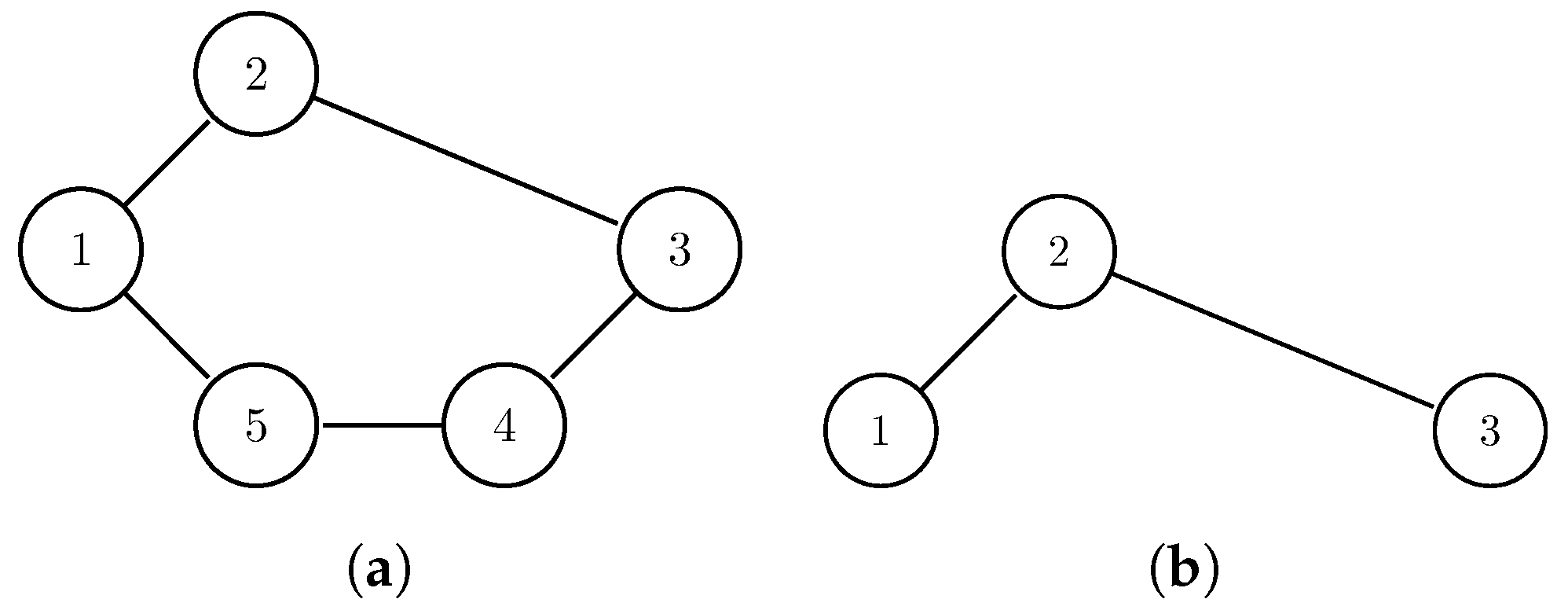
The definition of communities indicates that a certain RSM is required. We have shown that SDF is RSMFTN in Example 1, so that SDF is RSM. Although many community detection algorithms work on SDF, they may not always give a reasonable result. Intuitively, the relation of a pair of nodes will get stronger if there are more paths between them. However, the SDF does not consider this case (see Figure 4). More specifically, in SDF view, the relation will not get stronger unless a path shorter than the previous shortest path is added.

To avoid this problem, we use the Klein and Randic’s effective resistance function (ERF) [36] to measure the relation strength, which is later proved to be an RSM.

Suppose G is an indirectly connected graph. Then, G can be considered as an electrical network that all the edges are resistances with the corresponding weight values (if G is an unweighted graph, then the resistances of all edges are one). Let u and v be two vertices in the graph. Then, the effective resistance of these two vertices is

Definition 14.

Let the voltage of u be U and the one of v be 0. We can measure the current I from u to v. Then, the efficient resistance $R(u,v)$ between u and v is $\frac{U}{I}$. Briefly, $R(u,v)=\frac{U}{I}$.

Klein and Randic [36] provide an algorithm to compute the resistance distance for a connected indirect weighted graph. Suppose graph G is connected. Let A be the adjacent matrix and D the diagonal degree matrix of G. It is worth noting that, in a weighted undirected graph, the degree of a vertex is the sum of the weights of all its adjacent edges. Then, the Laplacian matrix L can be computed using formula $L=D-A$. Let $L^{†}$ be the generalized inverse [38] of L. Then, the efficient resistance distance $R_{i,j}$ of any pair of vertices $(i,j)$ in graph G can be obtained by

$$R_{i,j}=L_{i,i}^{†}+L_{j,j}^{†}-2L_{i,j}^{†},$$

and we usually call the corresponding matrix R resistance matrix.

Then, we show that ERF is an RSM. In this case, the relations among the nodes are derived from the electron flow in the wires among the vertices. Thus, we need to consider the criteria of RSMFTN.

Lemma 4.

Resistance is distance. That is, the resistance satisfies the following properties:

1. 

$R_{a,b}\ge 0,$

2. 

$R_{a,b}=0\iff a=b,$

3. 

$R_{a,b}=R_{b,a},$

4. 

$R_{a,c}+R_{c,b}\ge R_{a,b}.$

Lemma 5.

Let x be a cut-point of a connected graph, and let a and b be points occurring in different components which arise upon deletion of x. Then,

$$R_{a,b}=R_{a,x}+R_{x,b}.$$

Remark 9.

The proofs of Lemmas 4 and 5 have been given by Klein and Randic [36].

Lemma 6.

RDF satisfies property 5 of RSM.

Proof. 

Suppose G is some graph and $G^{\prime }$ is the same as G but the edges weights in $G^{\prime }$ are all $\alpha$ times greater than the ones in G. Let A and $A^{\prime }$ be the adjacent matrices of G and $G^{\prime }$, respectively. Then, we have $A^{\prime }=\alpha A$. Thus, for the corresponding degree matrices D and $D^{\prime }$, we also have $D^{\prime }=\alpha D$. Therefore, we have

$$L^{\prime }=D^{\prime }-A^{\prime }=\alpha D-\alpha A=\alpha (D-A)=\alpha L.$$

Let $L^{†}$ and $L^{\prime †}$ be the generalized inverse of L and $L^{\prime }$, respectively. Then, by the definition of the generalized inverse, we have

$$L{L}^{†}L=L,$$

(1)

$$L^{\prime }{L}^{\prime †}{L}^{\prime }=L^{\prime }.$$

(2)

Since $L^{\prime }=\alpha L$, we can simplify Equation 2 as

$$\begin{array}{c}{L}^{\prime }{L}^{\prime †}{L}^{\prime }=L^{\prime }\iff (\alpha L)L^{\prime †}(\alpha L^{\prime })=(\alpha L^{\prime })\iff L(\alpha L^{\prime †})L=L.\hfill \end{array}$$

Comparing with Equation (1), $\alpha L^{\prime †}$ has the same function as $L^{†}$. Since the final result does not rely on the choice of the generalized inverse matrix, we can let $L^{†}$ be the one satisfying the equation

$$\alpha L^{†}=L^{\prime †}.$$

(3)

Hence, we have

$$\begin{array}{cc}\hfill R_{i,j}^{\prime }& =L_{i,i}^{\prime †}+L_{j,j}^{\prime †}-2L_{i,j}^{\prime †}=\alpha L^{†}+\alpha L^{†}-2\alpha L^{†}\hfill \\ & =\alpha (L_{i,i}^{†}+L_{j,j}^{†}-2L_{i,j}^{†})=\alpha R_{i,j}.\hfill \end{array}$$

□

Proposition 1.

ERF is an RSMFTN.

Proof. 

We can define that the resistance distance of a pair of vertices is infinite if there is no path between them. Then, the proposition follows immediately from Lemmas 4–6. □

Therefore, ERF is RSM.

5.2. Community Detection in Zachary’s Karate Club

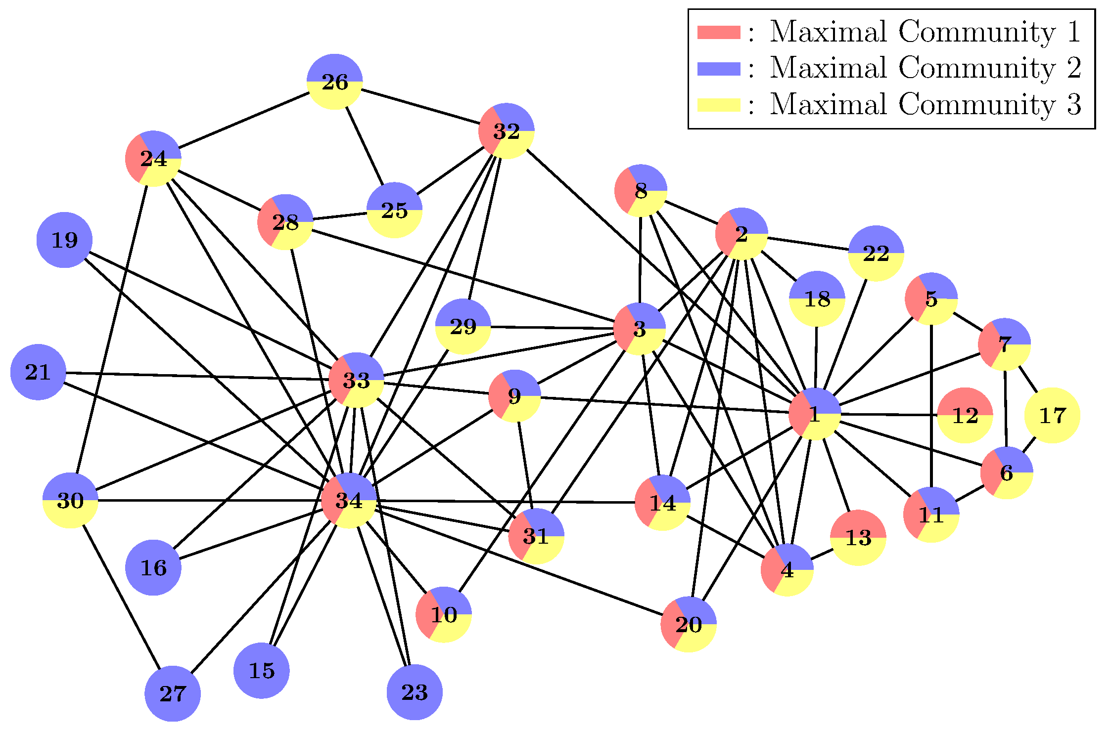
The graph we use for demonstration is Zachary’s karate club (Figure 5) [35], which is a popular test case in the community detection research. At first, we need to choose some proper CP, which is the lower bound of the relation strength within the communities. Here, we let $CP=1.5$. Then, we use the Klein–Randic method to compute the resistance distance for each pair of nodes in the network and get the corresponding resistance matrix R. After that, we get the corresponding adjoint graph (adj) from R and remove all the edges whose weights are greater than CP. Thus, we get the efficient edges graph (eeg). Then, we apply the Bron–Kerbosch algorithm on eeg and get a list of maximal communities. In Figure 5, we plot those maximal communities in the original graph. Here, we have three maximal communities represented by red, blue and yellow, respectively. Some nodes are multi-colour, which means they belong to various maximal communities simultaneously.

5.3. Comparison Results

We compare our algorithm with some popular ones that can generate communities with overlaps. We test them over LFR benchmark networks and calculate the normalized mutual information (NMI). In addition, we also provide some node-level performance measurement results: precision, recall and F-Score, which are defined as follows [39].

Let $C_s$ denote the set of communities generated by the LFR benchmark tests and $C_r$ the one generated by the testing algorithm. Based on $C_s$ and $C_r$, we first define two sets of node pairs:

$$\begin{array}{c}{O}_s=\{(u,v)|\mathrm{there}\mathrm{exists}\mathrm{a}\mathrm{community}\mathrm{in}{C}_s\mathrm{that}\mathrm{contains}(u,v)\},\mathrm{and}\hfill \\ O_r=\{(u,v)|\mathrm{there}\mathrm{exists}\mathrm{a}\mathrm{community}\mathrm{in}{C}_r\mathrm{that}\mathrm{contains}(u,v)\}.\hfill \end{array}$$

Then, we have

$$\begin{array}{ccc}\mathit{precision}=\frac{|O_s\cap O_r|}{|O_s|}\hfill & \mathrm{and}\hfill & \mathit{recall}=\frac{|O_s\cap O_r|}{|O_r|}.\hfill \end{array}$$

In addition, F-Score, an indicator for the quality of the tested algorithm’s solution, is

$$\mathit{F}-\mathit{Score}=2\times \frac{precision\times recall}{precision+recall}.$$

(4)

Note that NMI, precision, recall and F-Score all have the range between zero and one. Their values have a positive relationship with the quality of the community detection results. That is, closer-to-one scores imply a better detection solution.

Figure 6 plots the test results of our algorithm as well as the Community Overlap Propagation Algorithm (COPRA) [40], Connected Iterative Scan (CIS) [41], CFinder [42], Link [43] and Greedy Clique Expansion (GCE) [44]. In our experiments, we apply a similar configuration used by Xie et al. [45]. In particular, the LFR benchmark networks contain 100 nodes for each instance. The node degree, governed by the power laws with exponent two, has an average of six and maximum 50. The community size, ranging from 20 to 100, also follows a power law but with exponent one. For a node, the expected fraction of links that connect to other communities is set to $0.3$. We let ten percent of the nodes be shared by ${\mathcal{N}}_c$ various communities, where ${\mathcal{N}}_c=2,3,\cdots 8$. Since, in our algorithm, a pre-specified CP is required, we simply use the CP that gives the best performance.

From Figure 6, we can observe that our algorithm has a competitive NMI. The F-score of our algorithm, like others, has a negative relationship with ${\mathcal{N}}_c$. However, it still has a better performance. Remarkably, when ${\mathcal{N}}_c$ equals two, the average F-score of our algorithm is around $0.9$, which implies that the algorithm has found almost all local community structures. As ${\mathcal{N}}_c$ increases, compared with other methods, our method maintains a higher score until ${\mathcal{N}}_c=8$.

6. Conclusions

In this paper, we propose a general scheme to derive community detection algorithms. We mainly focus on two types of networks: transmission networks and similarity networks. For the networks belonging to each type, we discuss their shared properties and how to abstract a node-edge graph model from a practical network. In addition, we also discuss the relations between these two network types. Based on this, we report a general method to define community structures and derive a corresponding detection algorithm. Finally, we provide a demonstration to show how our scheme works. The experimental results show that an algorithm derived from our scheme can generate reasonable community detection results.

References

- Fortunato, S. Community detection in graphs. Phys. Rep. 2010, 486, 75–174. [Google Scholar] [CrossRef] [Green Version]
- Porter, M.; Onnela, J.; Mucha, P. Communities in networks. Not. Am. Math. Soc. 2009, 56, 1082–1097. [Google Scholar]
- Newman, M.E.J. Communities, modules and large-scale structure in networks. Nat. Phys. 2012, 8, 25–31. [Google Scholar]
- Kernighan, B.W.; Lin, S. An Efficient Heuristic Procedure for Partitioning Graphs. Bell Syst. Tech. J. 1970, 49, 291–307. [Google Scholar] [CrossRef]
- Hastie, T.; Tibshirani, R.; Friedman, J. The Elements of Statistical Learning, 2nd ed.; Springer: New York, NY, USA, 2009; pp. 520–523. [Google Scholar]
- Hlaoui, A.; Wang, S. A direct approach to graph clustering. Neural Netw. Comput. Intell. 2004, 4, 158–163. [Google Scholar]
- Rattigan, M.J.; Maier, M.; Jensen, D. Graph Clustering with Network Structure Indices. In Proceedings of the 24th International Conference on Machine Learning, Corvallis, OR, USA, 20–24 June 2007; pp. 783–790. [Google Scholar]
- Barnes, E.R. An Algorithm for Partitioning the Nodes of a Graph. In Proceedings of the 20th IEEE Conference on Decision and Control including the Symposium on Adaptive Processes, San Diego, CA, USA, 16–18 December 1982; pp. 541–550. [Google Scholar]
- Luxburg, U. A Tutorial on Spectral Clustering. Stat. Comput. 2007, 17, 395–416. [Google Scholar] [CrossRef]
- Li, Y.; He, K.; Kloster, K.; Bindel, D.; Hopcroft, J. Local Spectral Clustering for Overlapping Community Detection. ACM Trans. Knowl. Discov. Data 2018, 12, 1–27. [Google Scholar] [CrossRef]
- Lu, Z.; Wahlström, J.; Nehorai, A. Community Detection in Complex Networks via Clique Conductance. Sci. Rep. 2018, 8, 5982. [Google Scholar] [CrossRef] [Green Version]
- Newman, M.E. Fast algorithm for detecting community structure in networks. Phys. Rev. E 2004, 69, 066133. [Google Scholar] [CrossRef] [Green Version]
- Chen, M.; Kuzmin, K.; Szymanski, B.K. Community Detection via Maximization of Modularity and Its Variants. IEEE Trans. Comput. Soc. Syst. 2014, 1, 46–65. [Google Scholar] [CrossRef] [Green Version]
- Kaur, M.; Mahajan, A. Community Detection in Complex Networks: A Novel Approach Based on Ant Lion Optimizer. In Proceedings of the International Conference on Soft Computing for Problem Solving; Springer: Singapore, 2016; pp. 22–34. [Google Scholar]
- Reichardt, J.; Bornholdt, S. Detecting Fuzzy Community Structures in Complex Networks with a Potts Model. Phys. Rev. Lett. 2004, 93, 218701. [Google Scholar] [CrossRef] [PubMed]
- Wan, C.; Peng, S.; Wang, C.; Yuan, Y. Communities Detection Algorithm Based on General Stochastic Block Model in Mobile Social Networks. In Proceedings of the 2016 International Conference on Advanced Cloud and Big Data (CBD), Chengdu, China, 13–16 August 2016. [Google Scholar]
- Bickel, P.J.; Chen, A. A nonparametric view of network models and Newman-Girvan and other modularities. Proc. Natl. Acad. Sci. USA 2009, 106, 21068–21073. [Google Scholar] [CrossRef] [PubMed] [Green Version]
- Airoldi, E.M.; Blei, D.M.; Fienberg, S.E.; Xing, E.P. Mixed Membership Stochastic Blockmodels. In Proceedings of the International Conference on Neural Information Processing Systems (NIPS), Vancouver, BC, Canada, 8–10 December 2008. [Google Scholar]
- Wahlstrom, J.; Skog, I.; Rosa, P.S.L.; Handel, P.; Nehorai, A. The β-Model–Maximum Likelihood, Cramer–Rao Bounds, and Hypothesis Testing. IEEE Trans. Signal Process. 2017, 65, 3234–3246. [Google Scholar] [CrossRef]
- Milo, R.; Shen-Orr, S.; Itzkovitz, S.; Kashtan, N.; Chklovskii, D.; Alon, U. Network Motifs: Simple Building Blocks of Complex Networks. Science 2002, 298, 824–827. [Google Scholar] [CrossRef] [PubMed] [Green Version]
- Yaveroğlu, Ö.N.; Malod-Dognin, N.; Davis, D.; Levnajic, Z.; Janjic, V.; Karapandza, R.; Stojmirovic, A.; Pržulj, N. Revealing the Hidden Language of Complex Networks. Sci. Rep. 2014, 4, 4547. [Google Scholar] [CrossRef] [PubMed] [Green Version]
- Benson, A.R.; Gleich, D.F.; Leskovec, J. Higher-order organization of complex networks. Science 2016, 353, 163–166. [Google Scholar] [CrossRef] [PubMed] [Green Version]
- Bu, Z.; Li, H.; Cao, J.; Wang, Z.; Gao, G. Dynamic Cluster Formation Game for Attributed Graph Clustering. IEEE Trans. Cybern. 2019, 49, 328–341. [Google Scholar] [CrossRef]
- Newman, M.E.J. Equivalence between modularity optimization and maximum likelihood methods for community detection. Phys. Rev. E 2016, 94, 052315. [Google Scholar] [CrossRef] [Green Version]
- Li, H.; Bu, Z.; Li, A.; Liu, Z.; Shi, Y. Fast and Accurate Mining the Community Structure: Integrating Center Locating and Membership Optimization. IEEE Trans. Knowl. Data Eng. 2016, 28, 2349–2362. [Google Scholar] [CrossRef]
- Li, H.J.; Bu, Z.; Li, Y.; Zhang, Z.; Chu, Y.; Li, G.; Cao, J. Evolving the attribute flow for dynamical clustering in signed networks. Chaos Solitons Fractals 2018, 110, 20–27. [Google Scholar] [CrossRef]
- Li, H.; Bu, Z.; Wang, Z.; Cao, J.; Shi, Y. Enhance the Performance of Network Computation by a Tunable Weighting Strategy. IEEE Trans. Emerg. Top. Comput. Intell. 2018, 2, 214–223. [Google Scholar] [CrossRef]
- Peel, L.; Larremore, D.B.; Clauset, A. The ground truth about metadata and community detection in networks. Sci. Adv. 2017, 3, e1602548. [Google Scholar] [CrossRef] [PubMed] [Green Version]
- Guimera, R.; Mossa, S.; Turtschi, A.; Amaral, L.A.N. The worldwide air transportation network: Anomalous centrality, community structure, and cities’ global roles. PNAS 2005, 102, 7794–7799. [Google Scholar] [CrossRef] [PubMed]
- Chen, J.; Yuan, B. Detecting Functional Modules in the Yeast Protein–protein Interaction Network. Bioinformatics 2006, 22, 2283–2290. [Google Scholar] [CrossRef]
- Scholkopf, B.; Platt, J.; Hofmann, T. Fundamental Limitations of Spectral Clustering. In Proceedings of the International Conference on Neural Information Processing Systems (NIPS), Vancouver, BC, Canada, 3–6 December 2007. [Google Scholar]
- Li, H.J.; Daniels, J.J. Social significance of community structure: Statistical view. Phys. Rev. E 2015, 91, 012801. [Google Scholar] [CrossRef] [PubMed]
- Bron, C.; Kerboscht, J. Finding All Cliques of an Undirected Graph. Commun. ACM 1973, 16, 575–577. [Google Scholar] [CrossRef]
- Eppstein, D.; Löffler, M.; Strash, D. Listing All Maximal Cliques in Sparse Graphs in Near-Optimal Time. In Algorithms and Computation; Springer: Berlin/Heidelberg, Germany, 2010; pp. 403–414. [Google Scholar]
- Zachary, W. An information flow model for conflict and fission in small groups. J. Anthropol. Res. 1977, 33, 452–473. [Google Scholar] [CrossRef]
- Klein, D.J.; Randic, M. Resistance distance. J. Math. Chem. 1993, 12, 81–95. [Google Scholar] [CrossRef]
- Lancichinetti, A.; Fortunato, S.; Radicchi, F. Benchmark graphs for testing community detection algorithms. Phys. Rev. E 2008, 78, 046110. [Google Scholar] [CrossRef] [Green Version]
- Wong, E.T. Generalised Inverses as Linear Transformations. Math. Gaz. 1979, 63, 176–181. [Google Scholar] [CrossRef]
- Yang, T.; Jin, R.; Chi, Y.; Zhu, S. Combining link and content for community detection: A discriminative approach. In Proceedings of the 15th ACM SIGKDD International Conference on Knowledge Discovery and Data Mining, Paris, France, 28 June–1 July 2009; pp. 927–936. [Google Scholar]
- Gregory, S. Finding overlapping communities in networks by label propagation. New J. Phys. 2010, 12, 103018. [Google Scholar] [CrossRef] [Green Version]
- Baumes, J.; Goldberg, M.K.; Krishnamoorthy, M.; Magdon-Ismail, M.; Preston, N. Finding communities by clustering a graph into overlapping subgraphs. In Proceedings of the IADIS International Conference on Applied Computing, Algarve, Portugal, 22–25 February 2005. [Google Scholar]
- Adamcsek, B.; Palla, G.; Farkas, I.J.; Derényi, I.; Vicsek, T. CFinder: Locating Cliques and Overlapping Modules in Biological Networks. Bioinformatics 2006, 22, 1021–1023. [Google Scholar] [CrossRef] [PubMed]
- Ahn, Y.Y.; Bagrow, J.P.; Lehmann, S. Link communities reveal multiscale complexity in networks. Nature 2010, 466, 761–764. [Google Scholar] [CrossRef] [PubMed]
- Lee, C.; Reid, F.; McDaid, A.F.; Hurley, N.J. Detecting highly overlapping community structure by greedy clique expansion. In Proceedings of the ACM SIGKDD International Conference on Knowledge Discovery and Data Mining, Washington, DC, USA, 25–28 July 2010. [Google Scholar]
- Xie, J.; Szymanski, B. Towards Linear Time Overlapping Community Detection in Social Networks. Adv. Knowl. Discov. Data Min. 2012, 7302, 25–36. [Google Scholar] [Green Version]
Figure 1.
A typical speed function of time associated with node pair .
Figure 2.
Two nodes (u and v) connected by a single path (a) and two parallel paths (b).
Figure 3.
The concept graph of the algorithm.
Figure 4.
In both (a,b), the shortest distance between Node 1 and Node 3 is 2. Thus, in SDF’s view, the relation strengths between Node 1 and Node 3 in these two cases are identical. However, there is one more path between Node 1 and Node 3 in (a). Thus, intuitively, the relation between Node 1 and Node 3 in (a) should be stronger than the one in (b).
Figure 5.
Zachary’s karate club and its maximal communities by choosing .
Figure 6.
The NMI, Precision, Recall and F-Score of our algorithm, COPRA, CIS, CFinder, Link and GCE as a function of the number of communities by which a node is shared ().
© 2019 by the authors. Licensee MDPI, Basel, Switzerland. This article is an open access article distributed under the terms and conditions of the Creative Commons Attribution (CC BY) license (http://creativecommons.org/licenses/by/4.0/).
Share and Cite
MDPI and ACS Style
Lu, H.; Nayak, A. A Scheme to Design Community Detection Algorithms in Various Networks. Future Internet 2019, 11, 41. https://doi.org/10.3390/fi11020041
AMA Style
Lu H, Nayak A. A Scheme to Design Community Detection Algorithms in Various Networks. Future Internet. 2019; 11(2):41. https://doi.org/10.3390/fi11020041
Chicago/Turabian StyleLu, Haoye, and Amiya Nayak. 2019. "A Scheme to Design Community Detection Algorithms in Various Networks" Future Internet 11, no. 2: 41. https://doi.org/10.3390/fi11020041
Note that from the first issue of 2016, this journal uses article numbers instead of page numbers. See further details here.