The Whole Is Greater than the Sum of the Parts: A Multilayer Approach on Criminal Networks ^†

Abstract

Traditional social network analysis can be generalized to model some networked systems by multilayer structures where the individual nodes develop relationships in multiple layers. A multilayer network is called multiplex if each layer shares at least one node with some other layer. In this paper, we built a unique criminal multiplex network from the pre-trial detention order by the Preliminary Investigation Judge of the Court of Messina (Sicily) issued at the end of the Montagna anti-mafia operation in 2007. Montagna focused on two families who infiltrated several economic activities through a cartel of entrepreneurs close to the Sicilian Mafia. Our network possesses three layers which share 20 nodes. The first captures meetings between suspected criminals, the second records phone calls and the third detects crimes committed by pairs of individuals. We used measures from multilayer network analysis to characterize the actors in the network based on their local edges and their relevance to each specific layer. Then, we used measures of layer similarity to study the relationships between different layers. By studying the actor connectivity and the layer correlation, we demonstrated that a complete picture of the structure and the activities of a criminal organization can be obtained only considering the three layers as a whole multilayer network and not as single-layer networks. Specifically, we showed the usefulness of the multilayer approach by bringing out the importance of actors that does not emerge by studying the three layers separately.

1. Introduction

1.1. Contextualization

A long time before the development of social network analysis (SNA), people dealt with multiple social networks. Even if this has always been done with no effort, it is not a trivial activity that can be overlooked. One of the possible views of the problem is represented by the connections between individuals through multiple types of relational ties [1,2,3,4].

The world cannot be defined considering different kinds of relationships as ontologically equivalent and without taking into consideration the interactions among different kinds of connections from which invisible relationships emerge. For this reason, we cannot look only at a single kind of relationship within a single social network [1,2,3,4].

A single-layer perspective has been used to study the social interactions in most cases. These interactions have been measured for a long time through the simple graph, which is one of the most powerful tools from SNA. A simple graph is defined as a set of nodes with edges between them. There are no edges that connect a node to itself [2]. Nodes are often called actors, which usually represent individuals or organizations. Edges are also known as connections or links, and they usually represent relationships between individuals such as friendships. The type of graph is defined by edge weight and directionality. If there exists a numerical value (i.e., a weight) attached to each edge, then the graph is weighted. If all edges are bidirectional, then the graph is called undirected. If edges have directionality, then the graph is called directed.

In practical contexts, the most applied set of SNA tools is probably represented by the family of centrality measures. Centrality is an intrinsically relational concept. In fact, an actor needs to have relations to be important [2]. An actor is important if it is connected to other important nodes or to a large number of different nodes. An actor can also be central if his absence breaks the network into many isolated components. The position of the actor within a network can give him power in terms of the control over the information flowing through the network. The number of interactions of each actor is quantified by the most traditional centrality measure, which is the degree.

Social networks are usually treated as monodimensional objects, but they can at least have three different dimensions: (i) a structural dimension, (ii) a compositional dimension and (iii) an affiliation dimension. The full complexity of a social structure can be understood only through these dimensions [1]. The first one corresponds to the simple graph made by actors and their relationships. The second one describes the actors and their personal information. The third one indicates the belonging of these actors to the same organization or family.

Multiple relationships can also be considered according to an alternative conceptual approach as a set of layers (i.e., connected levels) [2,3,4]. Each simple graph with nodes and edges can be organized into multiple layers. Each layer can represent different types of edges, nodes, online social networks, communities, social contexts, and so on. In such a multilayer network, nodes in the different layers refer to a global set of actors, and edges can also connect nodes in the same layer (i.e., intralayer edges) or in different layers (i.e., interlayer edges). Analyzing multiple layers, we can obtain information that is not present in each single layer and would not be achieved considering layers independently of each other.

Many relevant works on multilayer networks have been reviewed and discussed by Kivelä et al. [5], who also presented a general framework for these kinds of networks [6,7,8]. This framework introduced the cumulative constraints on the general model [9], explaining the different types of networks: monoplex or single layer [6], multiplex [10,11,12], interdependent, and networks of networks.

Dickison, Magnani and Rossi [2] realized a book on the evolution of interconnected social networks, dynamic processes, data collection, data analysis, modeling and mining of multilayer social network systems. According to the authors, we can find multilayer social networks in different contexts. They are generated from data of different sizes, natures and layer semantics. More specifically, during SNA studies, many multilayer networks with actors connected by multiple types of edges have been created from offline questionnaires or interviews. They are often networks of small sizes, and they can be very useful in testing new methods. The only multilayer criminal network is the one described by Bright et al. [13]. This network has eight layers with a specific type of edge related to the exchange of drugs, money and other particular resources. The authors explored the actor’s strategic positions across the eight layers. They recognized the importance of multiplex data in criminal network analysis, but their results were limited to an aggregate network, which was obtained by summing up all interactions across the whole network while neglecting the layered structure.

1.2. Related Works

SNA in an essential tool to study criminal networks [14,15]. It can be used in many ways: (i) to describe the structure and functioning of criminal organizations [16,17]; (ii) to identify leaders within a criminal network [18,19,20,21,22,23]; (iii) to construct crime prevention systems [24,25]; (iv) to evaluate police interventions aimed at dismantling and disrupting criminal networks [26,27,28,29].

In 1991, Sparrow [30] began to explore and introduce the relevance of some concepts from the social network analysis such as centrality, equivalence and weak ties for the analysis of criminal intelligence. The notion of centrality refers to the use of standard centrality metrics from SNA to identify the key actors for a criminal organization. The concept of equivalence refers to the presence in the criminal network of individuals with similar roles or with the same neighborhood. Weak ties are connections among actors who have no other direct connections. Sparrow also identified the three main problems of criminal network analysis: (i) incompleteness (i.e., missing nodes and edges); (ii) fuzzy boundaries (i.e., which individuals to include and which not to include in the network); (iii) dynamic (i.e., criminal networks are not static, but they change over time).

Klerks [31] described a crisis of LEA confidence in the mid-1990s which led to a collaboration between Dutch law enforcement and academics to develop elaborate network approaches to organized crime. Thanks to this collaboration, it was possible to identify powerful positions inside criminal networks and to attribute these positions to specific individual traits or to structural roles covered by these individuals. For example, the centrality of intermediaries was recognized because these figures could monopolize the connection inside criminal networks. Moreover, according to the author, valuable resources and information for criminals could be discovered thanks to social network mapping.

Xu and Chen [17] studied the topology of criminal networks, which are characterized by a high clustering coefficient, a short average path length and a high level of efficiency in terms of communication, information flow and commands. These networks are moreover more vulnerable to attacks when the targets are the bridges connecting different communities within them rather than their high-degree nodes.

Van der Hulst [14] offered a general introduction to SNA as an analytical tool for the study of criminal networks, whose systematic analysis could lead to a more comprehensive understanding of criminal behavior. Some theoretical and key concepts were reviewed by the author together with functional applications, and a tentative protocol for coding and data handling.

Morselli [16] wrote an excellent book applying a social network perspective to a variety of illegal enterprises, focusing on the flexibility of these organizations and their strategies to adjust after losing key members or opportunities. The author examined the structures and dynamics of criminal networks, their key and peripheral players, their balance between efficiency and security, positions and individual traits, the use of legitimate actors in illegal settings, and finally the network adaptation against disruption.

Calderoni [32] discussed the state of the art in the study of organized criminal groups through the application of SNA methods. He used both the academic and law enforcement perspectives to provide an overview of the field development and to describe the existing approaches. The author focused on data sources, the type of network analysis, and the limitations due to the application of SNA to criminal organizations. He also identified the future trends and suggested some promising paths from both a policy and research perspective.

Berlusconi [33] also highlighted the relevance of SNA to analyze criminal groups, for both research and LEA purposes. She discussed how SNA can be applied in various areas related to the criminological context, and how this application could have great value for crime prevention.

Burcher [34] explained how intelligence analysts apply SNA in operational environments focusing on the identification of key actors, network vulnerabilities, avenues of enquiry, link and attribute weights, and when during an investigation, analysts apply SNA.

Bright et al. [35] discussed the growth in popularity of the use of SNA to study crime and reviewed the challenges related to the use of data extracted from criminal justice records. They offered to researchers some recommendations about data collection and preparation when utilizing these kinds of records. The use of criminal justice records can suffer from a number of limitations in terms of accuracy, validity and reliability. Such data may suffer from the problem of missing data. They may include transcription errors, aliases or false information. The authors also outlined and discussed the different types of data used across this literature.

1.3. Past Approaches

In [36], we proposed a unique multilayer mafia network. The Sicilian Mafia [37,38] is one of the most renowned criminal organizations. Each mafia group is called a cosca, family or clan. The analysis of the mafia social structure inspired great interest in the scientific community [39]. Our multilayer network was built from two simple graphs that captured the meetings and phone calls between a couple of suspected criminals identified by police audio and physical surveillance during an anti-mafia operation known as Montagna [25,29,40]. The Public Prosecutor’s Office of Messina (Sicily) concluded this investigation in 2007. Given these two single-layer networks, we build a weighted and undirected multilayer network with 154 actors, 439 intralayer edges, and 2 layers named Meetings and Phone Calls. Then, we focused on the identification of leaders within the two-layer Montagna network. We chose the degree as descriptor to identify the 20 most important actors in the network. We used three different approaches to compute degree: (i) on each layer separately, according to its standard definition on simple graphs; (ii) on the aggregated network obtained by merging the two layers of the multilayer network into a single-layer network, again according to its standard definition; and (iii) on the multilayer network, computed as the number of each actor’s relational ties on all the layers in which he exists.

In this paper, which is an extended version of [36], we rebuilt the multilayer network adding a third layer derived by a third new simple graph based on the crimes that suspected criminals from the Montagna operation committed together. The resulting network is a weighted and undirected multilayer network with 226 actors, 454 intralayer edges, and 3 layers named Meetings, Phone Calls and Crimes. Then, we made a deep study of the new three-layer Montagna network using at first some traditional measures from SNA to study the single layers and, then, actor and layer measures from the multilayer network analysis to evaluate the actor importance in each layer and in the whole structure and the dissimilarity among the layers. To the best of our knowledge, we are the first to build and study a criminal network in a form of multilayer network and not as an aggregate network. From our analysis, a different understanding of the network structure and of the key actors emerges, which allows to declare that LEAs should collect more multiplex data in order to reduce their efforts during an investigation. The identification of key actors taking into account more layers could, in fact, better identify the strategic positions of suspected criminals allowing to make decisions on targets of surveillance or arrest.

2. Materials and Methods

2.1. Multilayer Networks

A multilayer network is the most general structure to represent any kind of network [5]. The elementary concept of a graph, also known as single-layer network, is at the base of its structure.

Definition 1

(Single-layer network). A single-layer network is defined as a simple graph [1] $G=(V,E)$ where $V=\{v_1,v_2,\dots ,v_N\}$ is the set of nodes and $E=\{l_1,l_2,\dots ,l_L\}$, $E\subseteq V\times V$ is the set of edges.

Networks with multiple levels, multiple types of edges or other similar features can be represented, adding some structures with layers to nodes and edges.

Definition 2

(Multilayer network). A multilayer network [2] is defined as a quadruple $M=(\mathcal{A},\mathcal{L},V,E)$, where $\mathcal{A}$ is the set of actors, $\mathcal{L}$ is the set of layers, $(V,E)$ is a simple graph and $V\subseteq \mathcal{A}\times \mathcal{L}$.

An actor is the real-world concept represented by a node which is an element of the mathematical concept of the graph. An actor can be a person, an organization or an entity which has relationships with other actors. The same actor can be present in different layers, where each layer represents a type of actor or a type of edge between actors. A node represents a specific actor on a specific layer (e.g., a node can be the Facebook or Twitter account of a specific user which is the actor). Using multiple layers, we can represent different types of edges that correspond to the relationships between nodes. Intralayer edges are those among nodes in the same layer. Interlayer edges are those among nodes in different layers.

When a common set of actors is connected through multiple types of edges, a multilayer network can be reduced to a multiplex network.

Definition 3

(Multiplex network). A multiplex network [5] can be defined as a sequence of graphs ${\left\{G_{\alpha }\right\}}_{\alpha =1}^b={\left\{(V_{\alpha },E_{\alpha })\right\}}_{\alpha =1}^b$, where $E_{\alpha }\subseteq V_{\alpha }\times V_{\alpha }$ is the set of edges and α is the index for the graphs and usually ${\bigcap }_{\alpha =1}^b{V}_{\alpha }\ne \varnothing$ (i.e., the different layers at least share some nodes).

2.1.1. Descriptive Measures

One of the main approaches to study multilayer networks consists in applying typical measures of the traditional SNA to each layer separately and then comparing these results [2]. This kind of approach can be useful for producing an initial overview of the data before applying truly multilayer measures.

Different layers have in fact their specific characteristics in terms of number of nodes or edges, edge directionality, graph density, clustering coefficient, components, or network diameter when observed one at a time.

Definition 4

(Directionality). Edge directionality is a key property that defines the type of graph together with edge weight (i.e., a numerical value attached to each edge). If all edges are bidirectional, then the graph is called undirected. If edges have directionality, then the graph is called directed.

Definition 5

(Density). Graph density is a measure of how many edges between nodes exist compared to how many edges between actors are possible. It is defined as:

$$\delta =\frac{L}{N(N-1)}.$$

(1)

Definition 6

(Diameter). Graph diameter $d_{max}$ [41] is the maximum shortest path in the graph, where the shortest path (or distance) $d_{v_i{v}_j}$ between nodes $v_i$ and $v_j$ is the path with the fewest number of edges. A path is a sequence of nodes such that each node is connected to the next node along the path by an edge.

Definition 7

(Average path length). The average path length $\langle d\rangle$ [41] is the average distance between all pairs of nodes in the graph. It is defined as:

$$\langle d\rangle =\sum _{v_i,v_j\in V}\frac{d_{v_i{v}_j}}{N(N-1)}.$$

(2)

Definition 8

(Connected component). A connected component $cc$ [41] is a subset of nodes in a graph, so that there is a path between any two nodes that belongs to the component, but one cannot add any more nodes to it that would have the same property.

Definition 9

(Largest connected component). The largest or giant connected component $lcc$ can be found typically in real undirected graphs, and it contains most of the nodes in the graph. The rest of the graph usually is divided into a large number of small components disconnected from the others.

Definition 10

(Degree). The degree k [36] is a key property of each node in a graph and represents the number of connections it has to other nodes. It is defined as:

$$k\left(v_i\right)=\left|\{v_j:(v_i,v_j)\in E\vee (v_j,v_i)\in E\wedge v_i\ne v_j\}\right|.$$

(3)

Definition 11

(Degree distribution). The degree distribution $p_k$ [41] provides the probability that a randomly selected node $v_i$ in the graph has degree k. For a graph with N nodes, the degree distribution is a normalized histogram given by:

$$p_k=\frac{N_k}{N},$$

(4)

where $N_k$ is the number of nodes with degree equal to k.

Definition 12

(Average clustering coefficient). The average clustering coefficient $\langle C\rangle$ [41] is the probability that two neighbors of a randomly selected node link to each other. It is defined as:

$$\langle C\rangle =\frac{1}{N}\sum _1^{N}C\left(v_i\right),$$

(5)

where $C\left(v_i\right)$ is the clustering coefficient of a node $v_i$ which captures the degree to which the neighbors of $v_i$ link to each other. It is defined as:

$$C\left(v_i\right)=\frac{2L_i}{k\left(v_i\right)(k\left(v_i\right)-1)},$$

(6)

where $L_i$ represents the number of edges between the k neighbors of the node $v_i$.

2.1.2. Actor Measures

Actors in multilayer networks can be described by a specific set of metrics [2]. Some of them are direct extensions of their single-layer counterparts and measure actors based on their local edges and relationships. Other measures have no counterpart for single-layer networks. They characterize the relevance of a specific layer or set of layers within the context of the connectivity of the actors.

Definition 13

(Multilayer actor degree). Given a multilayer network $M=(\mathcal{A},\mathcal{L},V,E)$, the degree [2] of an actor $a\in \mathcal{A}$ on a set of layers $L\subseteq \mathcal{L}$ is the number of his connections on all these layers. It is defined as:

$$k(a,L)=\left|\{\{(a,l),(a^{\prime },l^{\prime })\}\in E:l,l^{\prime }\in L\}\right|.$$

(7)

When $L=\mathcal{L}$, the degree of the actor is within the whole multilayer network, whereas when the set of layers contains only one layer, the traditional degree is computed as shown in Equation (3) for the actor in that layer.

Definition 14

(Multilayer actor degree deviation). Given a multilayer network $M=(\mathcal{A},\mathcal{L},V,E)$, the degree deviation [2] of an actor $a\in \mathcal{A}$ on a set of layers $L\subseteq \mathcal{L}$ is defined as the standard deviation of the degree of a over the layers in L:

$${\sigma }_k=\sqrt{\frac{{\displaystyle \sum _{l\in L}}{\left(k(a,\left\{l\right\})-\frac{k(a,L)}{\left|L\right|}\right)}^2}{\left|L\right|}}.$$

(8)

The degree deviation indicates the presence of an actor in the multilayer network and quantifies to what extent actors have similar or different degrees on the different layers.

Definition 15

(Multilayer actor neighborhood). Given a multilayer network $M=(\mathcal{A},\mathcal{L},V,E)$, the neighborhood [2] of an actor $a\in \mathcal{A}$ on a set of layers $L\subseteq \mathcal{L}$ is the number of the neighbors $ns$ of a, i.e., those distinct actors that are connected to a on a specific layer or set of layers. It is defined as:

$$n(a,L)=\left|\{a^{\prime }\in \mathcal{A}:\{(a,l),(a^{\prime },l^{\prime })\}\in E\wedge l,l^{\prime }\in L\}\right|=\left|ns(a,L)\right|.$$

(9)

When computed on a single layer network, degree and neighborhood coincide. However, the degree of an actor cannot be defined anymore as the number of adjacent actors in a multilayer network where actors can be connected to different individuals depending on the layer.

Definition 16

(Multilayer actor exclusive neighborhood). Given a multilayer network $M=(\mathcal{A},\mathcal{L},V,E)$, the exclusive neighborhood [2] of an actor $a\in \mathcal{A}$ on a set of layers $L\subseteq \mathcal{L}$ counts the neighbors that are adjacent to a only on the input layers L. It is defined as:

$$xn(a,L)=\left|ns\right(a,L) \backslash ns(a,\mathcal{L} \backslash L\left)\right|,$$

(10)

where the symbol \ indicates the set difference operation.

The exclusive neighborhood considers the actors that are connected exclusively on a specific layer or set of layers, and it is used to explore the role of specific layers for specific actors. If an actor has a high exclusive neighborhood on a layer, this means that this layer is important to maintain the actor connectivity. In fact, if the layer was removed, the actor’s neighbors would also disappear.

Definition 17

(Multilayer actor relevance). Given a multilayer network $M=(\mathcal{A},\mathcal{L},V,E)$, the relevance [2] of an actor $a\in \mathcal{A}$ on a set of layers $L\subseteq \mathcal{L}$ is the ratio between the neighbors of a on the specific set of layers L and the total number of his neighbors. It is defined as:

$$r(a,L)=\frac{n(a,L)}{n(a,\mathcal{L})}.$$

(11)

The relevance describes the specific signature of each actor, i.e., to be present on the different layers.

Definition 18

(Multilayer actor exclusive relevance). Given a multilayer network $M=(\mathcal{A},\mathcal{L},V,E)$, the exclusive relevance [2] of an actor $a\in \mathcal{A}$ on a set of layers $L\subseteq \mathcal{L}$ is the fraction of neighbors directly connected with a through edges belonging only to layers in L. It is defined as:

$$xr(a,L)=\frac{xn(a,L)}{xn(a,\mathcal{L})}.$$

(12)

The exclusive relevance measures what impact the removal of a specific layer or set of layers would have on the connectivity of an actor, also in this case in terms of neighbors.

2.1.3. Layer Measures

Actor measures such as the relevance can be used to know the role of a layer (or a set of layers) with respect to its actors. In order to know the relationship between different layers (or sets of layers), some measures of layer similarity need to be introduced. Layer similarity can be studied from two different perspectives: the actor-centered perspective and layer-centered perspective [2]. The first one describes the differences between different layers as a sign of different behaviors of the actors, strategically selecting what kinds of connections they want to establish on every layer. The second one describes the differences between layers in terms of interlayer influences, and it can be investigated by applying existing methods to compute correlation and similarities to multilayer networks.

Berlingerio et al. [42] developed the idea of layer correlation as a multilayer network version of the classical Jaccard correlation coefficient.

Definition 19

(Jaccard correlation coefficient). Given two finite sample sets A and B, the Jaccard correlation coefficient [43] is defined as the size of the intersection divided by the size of the union of the sample sets:

$$J(A,B)=\frac{|A\cap B|}{|A\cup B|}.$$

(13)

Definition 20

(Jaccard layer correlation coefficient). Given a multilayer network $M=(\mathcal{A},\mathcal{L},V,E)$, the Jaccard layer correlation coefficient [42] computes the ratio of pairs of actors connected on a set of layers $L\subseteq \mathcal{L}$ and the total number of pairs of actors connected in at least one layer in L. It is defined as:

$$J\left(L\right)=\frac{\left|{\bigcap }_{l\in L}{P}_l\right|}{\left|{\bigcup }_{l\in L}{P}_l\right|},$$

(14)

where $P_l$ denotes the set of pairs of actors connected in each layer $l\in L$.

The Jaccard coefficient can be used to measure the overlapping of the actors, i.e., the presence of common actors between pair of layers in a multilayer network.

This coefficient can also be used to measure the overlapping of the edges to know if the common actors between two layers behave in a similar way. This measure can show edges that actually exist in each pair of layers and actors that are highly connected on a layer but not on the other layer. If actors who are connected by an edge in one layer are also connected in the other layer, the value of edge overlapping will be equal to 0. On the contrary, this value will be 1 if the actors are connected in both layers or in none of the layers.

De Domenico et al. [8] introduced an actor-centered approach trying to quantify the similarity between the degree of actors across various layers. In this case, it is possible to use the Pearson correlation coefficient.

Definition 21

(Pearson correlation coefficient). Given two random variables a and b, the Pearson correlation coefficient [44] is defined as:

$$P_r=\frac{cov(a,b)}{{\sigma }_a{\sigma }_b},$$

(15)

where $cov(a,b)$ is the covariance of a and b and ${\sigma }_a{\sigma }_b$ is the product of their standard deviations.

Definition 22

(Pearson interlayer correlation coefficient). Given a multilayer network $M=(\mathcal{A},\mathcal{L},V,E)$, the Pearson correlation coefficient [12] is defined as:

$$P_r(l,l^{\prime })=\frac{\langle k(a,l)k(a,l^{\prime })\rangle -\langle k(a,l)\rangle \langle k(a^{\prime },l^{\prime })\rangle }{{\sigma }_{k(a,l)}{\sigma }_{k(a^{\prime },l^{\prime })}},$$

(16)

where $k(a,l)$ and $k(a^{\prime },l^{\prime })$ are the degrees of actor a, respectively, at layer l and layer $l^{\prime }$, and ${\sigma }_{k(a,l)}{\sigma }_{k(a^{\prime },l^{\prime })}$ is the product of their standard deviations.

For each pair (actor, layer), the Pearson correlation does not depend on the connected actors but only on the number of incident edges on an actor.

The difference between the degree distributions in different layers can instead been quantified using the Jeffreys dissimilarity function [45].

Definition 23

(Jeffreys dissimilarity function). The Jeffreys dissimilarity function [46] is a symmetrized relative entropy (i.e., a measure of the inherent uncertainty or randomness of a single random variable). Given two ensembles A and B, it is defined as:

$$D_J(A,B)=\frac{1}{2}\sum _{x}P\left(A_x\right)log\frac{P\left(A_x\right)}{P\left(B_x\right)}+\frac{1}{2}\sum _{x}P\left(B_x\right)log\frac{P\left(B_x\right)}{P\left(A_x\right)},$$

(17)

where $P\left(A_x\right)$ and $P\left(B_x\right)$ are the probabilities of the propositions $\left\{A_x\right\}$ and $\left\{B_x\right\}$ indexed by the sample space x.

Definition 24

(Jeffreys layer dissimilarity function). The Jeffreys layer dissimilarity function [47] is used to compare two layers as a distance between discrete distributions (e.g., the degree distribution) based on distance between histograms. It is defined as:

$$D_J(l,l^{\prime })=\sum _{k=1}^K{p}_k^{l}log\frac{p_k^l}{p_k^{l^{\prime }}}+\sum _{k=1}^K{p}_k{l}^{\prime }log\frac{p_k^{l^{\prime }}}{p_k^l},$$

(18)

where $p_k^l$ is the relative frequency of the kth degree value in a layer l.

Two layers are more dissimilar when Jeffreys divergence values are higher.

2.2. Multilayer Criminal Network Data

As already explained in Section 1.3, our dataset derives from the Montagna operation, which was an investigation carried out by R.O.S. (Special Operations Group), i.e., a specialized anti-mafia police unit of the Italian Carabinieri. This operation was concluded in 2007 by the Public Prosecutor’s Office of Messina, i.e., the third largest city on the island of Sicily (Italy).

The Montagna operation focused on the Mistretta family and the Batanesi clan, i.e., two mafia families who used a cartel of corrupted entrepreneurs to infiltrate the public works in the northeastern part of Sicily in the period 2003–2007. The Mistretta family also had a mediator role between two families known as Barcellona and Caltagirone, who operated around Messina, and other criminal organizations around Palermo and Catania.

On 14 March 2007, the Preliminary Investigation Judge of the Court of Messina issued a pre-trial detention order, which represents the main data source for our criminal networks. The pre-trial detention for 38 individuals was ordered by the court who wrote a document of more than two hundred pages containing a lot of details about meetings, phone calls, crimes and other activities among the suspects.

Two graphs were initially built from the analysis of this document: Meetings and Phone Calls [25,29,40]. The Meetings network is made of 101 nodes (i.e., suspected criminals) and 256 edges (i.e., meetings among couples of suspected criminals). The Phone Calls network is characterized by 100 nodes (i.e., suspected criminals) and 124 edges (i.e., phone calls among couples of suspected criminals). A total of 47 suspects jointly belongs to both networks.

In the current study, we also built a third graph called Crimes characterized by 25 nodes and 74 edges. It shares with the Meetings and Phone Calls graphs 20 nodes, which are also in this case suspected criminals. Individuals are connected by an edge if they have committed crimes together.

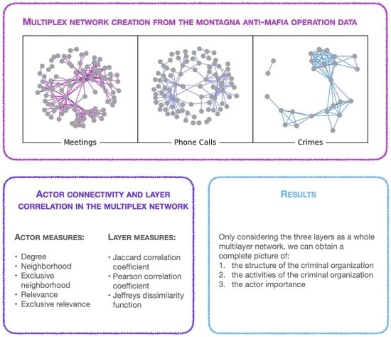
In our previous work [36], we created from the Meetings and Phone Calls graphs a weighted and undirected multilayer network with 154 actors, 439 intralayer edges and 2 layers. In this paper, we rebuilt the multilayer network adding the Crimes layer to the Meetings and Phone Calls layers (see Figure 1). Our new undirected and weighted multiplex network has 226 actors and 454 intralayer edges. Edges in the Meetings layer represent the meetings among suspected criminals; those in the Phone Calls layer refer to the phone communications among distinct phone numbers; those in the Crimes layer refer to common crimes committed by the members of the criminal network. The number of meetings, phone calls or common crimes are encoded by the edge weights. According to Definition 3, our network can be identified as a multiplex network. In fact, a multiplex network requires that each layer share at least one node with some other layer. In our case, Meetings and Phone Calls layers share 47 actors; Meetings and Crimes layers share 25 actors; and Phone Calls and Crimes layers share 20 actors.

2.3. Experimental Design

The analysis of our multiplex criminal network was conducted using the Python module uunet.multinet (available at: https://bitbucket.org/uuinfolab/py_multinet/src/master/, accessed on 10 April 2022) created by Magnani, Rossi and Vega to analyze multiplex social networks. This library is the Python version of the multinet library for the analysis of multilayer networks released by the same authors for the R framework [48].

Algorithm 1 shows the design of our experiments.

Algorithm 1: Multilayer approach.

We started with the creation of the three simple graphs Meetings ($G_1$), Phone Calls ($G_2$) and Crimes ($G_3$) described in Section 2.2, and we added them, respectively, as the first layer ($l_1$), second layer ($l_2$) and third layer ($l_3$) of a multiplex network M.

We applied to each layer l some of the most traditional SNA measures such as the number of nodes, number of edges, directionality, number of connected components, size of the largest connected component, density, clustering coefficient, average path length and diameter (see Section 2.1.1).

Then, we studied the actors in the network (see Section 2.1.2). We computed the highest degree actors on the whole multiplex network focusing on the 20 most central actors. We also compared the degree values of each actor in each specific layer computing the standard deviation of the degree. It can be a useful function to estimate what actors possess similar or different degrees on the various layers.

Given the set of the 20 most central actors $K_{\mathcal{A}}$, we computed the neighborhood for these actors considering the whole network with all the three layers ($\mathcal{L}$) and the exclusive neighborhood on each layer l. The neighborhood is not evaluated on each layer because on a single layer, neighborhood and degree have the same value. The exclusive neighborhood is calculated on a layer because it allows knowing if a layer is important to maintain the actor connectivity.

We also calculated relevance and exclusive relevance for the actors in $K_{\mathcal{A}}$ on each layer l. Relevance and exclusive relevance allow studying the relation between the multilayer network and the actors identifying those who are highly connected on a given layer or actors that are connected uniquely through a layer.

At the end, we compared layers using four different approaches (see Section 2.1.3). We computed the overlapping of actors and edges using the Jaccard correlation coefficient. Consequently, we determined the correlation between the degrees using the Pearson correlation coefficient to know if actors with a high degree on one layer had a similar behavior on the other layers. Then, we evaluated the dissimilarity between degree distributions using the Jeffreys dissimilarity function.

3. Results

Table 1. Descriptive measures for the flattened Montagna multiplex network and its three layers: number of nodes, number of edges, directionality, number of connected components, size of the largest connected component, density, clustering coefficient, average path length and diameter.

Layer	N	L	Dir.	$\left|\mathit{cc}\right|$	lcc	$\mathit{\delta }$	$\langle \mathit{C}\rangle$	$\langle \mathit{d}\rangle$	${\mathit{d}}_{max}$
Meetings ($l_1$)	101	256	False	5	92	0.050693	0.417647	3.308887	7
Phone Calls ($l_2$)	100	124	False	5	89	0.025051	0.072687	3.378192	7
Crimes ($l_3$)	25	74	False	2	23	0.246667	0.779626	2.407115	6

shows our preliminary analysis of the multiplex network considering each layer as an independent graph. The third layer is the smallest one and presents different characteristics especially in terms of number of connected components, size of the largest connected component and graph density. The first two layers seem to be more similar with the exception of the average clustering.

The results obtained applying the actor measures on the Montagna multiplex network are shown in Figure 2 and more in detail in

Table 2. Degree and degree deviation computed on the 20 highest-degree actors on the whole Montagna multiplex network and on its single layers.

a	$\mathit{k}(\mathit{a},\mathcal{L})$	$\mathit{k}(\mathit{a},{\mathit{l}}_1)$	$\mathit{k}(\mathit{a},{\mathit{l}}_2)$	$\mathit{k}(\mathit{a},{\mathit{l}}_3)$	${\mathit{\sigma }}_{\mathit{k}}$
18	57	24	25	8	7.788881
47	44	19	21	4	7.586538
27	31	16	11	4	4.921608
29	30	13	9	8	2.160247
61	29	4	17	8	5.436502
68	25	15	10	N/A	6.236096
54	24	6	5	13	3.559026
45	24	12	6	6	2.828427
51	22	11	4	7	2.867442
48	21	12	1	8	4.546061
64	18	6	2	10	3.265986
12	17	16	1	N/A	7.318166
22	16	14	2	N/A	6.182412
11	16	12	4	N/A	4.988877
75	15	4	8	3	2.160247
43	14	9	5	N/A	3.681787
36	14	8	4	2	2.494438
25	14	13	1	N/A	5.906682
63	13	4	1	8	2.867442
50	13	8	1	4	2.867442

,

Table 3. Neighborhood computed on 20 highest-degree actors of the whole Montagna multiplex network and exclusive neighborhood computed on its single layers.

a	$\mathit{n}(\mathit{a},\mathcal{L})$	$\mathit{xn}(\mathit{a},{\mathit{l}}_1)$	$\mathit{xn}(\mathit{a},{\mathit{l}}_2)$	$\mathit{xn}(\mathit{a},{\mathit{l}}_3)$
18	44	14	15	3
47	29	8	10	0
27	24	10	5	3
29	20	7	2	4
61	24	2	13	5
68	19	9	4	N/A
54	17	1	1	10
45	17	7	2	3
51	15	5	0	4
48	14	6	0	2
64	13	3	0	6
12	16	15	0	N/A
22	15	13	1	N/A
11	15	11	3	N/A
75	13	3	7	1
43	11	6	2	N/A
36	13	7	3	2
25	13	12	0	N/A
63	9	1	0	4
50	9	5	0	1

and

Table 4. Relevance and exclusive relevance of the 20 highest-degree actors on each layer of the Montagna multiplex network.

a	$\mathit{r}(\mathit{a},{\mathit{l}}_1)$	$\mathit{xr}(\mathit{a},{\mathit{l}}_1)$	$\mathit{r}(\mathit{a},{\mathit{l}}_2)$	$\mathit{xr}(\mathit{a},{\mathit{l}}_2)$	$\mathit{r}(\mathit{a},{\mathit{l}}_3)$	$\mathit{xr}(\mathit{a},{\mathit{l}}_3)$
18	0.545455	0.318182	0.568182	0.340909	0.181818	0.068182
47	0.655172	0.275862	0.724138	0.344828	0.137931	0.000000
27	0.666667	0.416667	0.458333	0.208333	0.166667	0.125000
29	0.650000	0.350000	0.450000	0.100000	0.400000	0.200000
61	0.166667	0.083333	0.708333	0.541667	0.333333	0.208333
68	0.789474	0.473684	0.526316	0.210526	N/A	N/A
54	0.352941	0.058824	0.294118	0.058824	0.764706	0.588235
45	0.705882	0.411765	0.352941	0.117647	0.352941	0.176471
51	0.733333	0.333333	0.266667	0.000000	0.466667	0.266667
48	0.857143	0.428571	0.071429	0.000000	0.571429	0.142857
64	0.461538	0.230769	0.153846	0.000000	0.769231	0.461538
12	1.000000	0.937500	0.062500	0.000000	N/A	N/A
22	0.933333	0.866667	0.133333	0.066667	N/A	N/A
11	0.800000	0.733333	0.266667	0.200000	N/A	N/A
75	0.307692	0.230769	0.615385	0.538462	0.230769	0.076923
43	0.818182	0.545455	0.454545	0.181818	N/A	N/A
36	0.615385	0.538462	0.307692	0.230769	0.153846	0.153846
25	1.000000	0.923077	0.076923	0.000000	N/A	N/A
63	0.444444	0.111111	0.111111	0.000000	0.888889	0.444444
50	0.888889	0.555556	0.111111	0.000000	0.444444	0.111111

.

Table 2 contains the degree of the 20 most central actors in the whole network and in each single layer. It also shows the standard deviation of the degree. Our actors are specific individuals involved in criminal activities or members of Mafia families which were at the center of the Montagna operation. We reconstructed the actor roles reading court documents of the anti-mafia operation. These roles have been analyzed in our previous work [36] making particular reference to the structure of a Mafia family which is characterized by typical figures such as boss, underboss, consigliere, messaggero, caporegimes, soldiers and associates. Considering the layered structure, the actors we identified as the most central are 18, 47 and 27. These actors are respectively a caporegime of the Mistretta family, a deputy caporegime and a caporegime of the Batanesi family. Therefore, they are effectively important. Caporegimes manage their crew of soldiers (i.e., average type criminals) within a Mafia family in a specific geographical location. These actors have similar degrees on the first two layers and different degrees on the third one. The Crimes layer does not include some of the most central actors such as 68, 12, 22, 11, 43 and 25. Actor 22 is a pharmacist which can be an important figure because chemical or pharmacological knowledge is required during a process of drug synthesis. Actor 11 is a criminal activity coordinator in Messina which is central to know the connection among the Mistretta and Batanesi families with other criminal organizations sited in Messina. Node 43 is the messaggero who is a key figure in a Mafia family who functions as a connection between families. He limits the boss exposure, reducing the necessity to meet publicly. Actor 29 seems to have equal importance for all the three layers as confirmed by a low degree deviation. He is an entrepreneur. Compared with the two-layer multiplex network described in [36], adding the third layer brings to light the importance of the entrepreneurs such as actors 54, 64 and 63, who did not appear as prominent figures from the analysis of the first two layers. Entrepreneurs are important Mafia associates because they can make the criminal organization win public tenders and accomplish the public contracts in a fraudulent way.

Table 3 shows, respectively, the neighborhood of the 20 highest-degree actors of the whole Montagna multiplex network and the exclusive neighborhood of the same actors on each layer of the network. Given an actor a, the neighborhood of a considers only the distinct actors who are connected to a within the whole multilayer network. As we can observe comparing the second columns of Table 2 and Table 3, some actors are connected on multiple layers. These actors will not have a higher neighborhood, but they will have a higher degree. A low exclusive neighborhood on a layer implies that a layer is not important to maintain the actor connectivity. If the Phone Calls layer disappeared, actors such as 51, 48, 64, 12, 25, 63, and 50 would lose 0 neighbors. This layer is not essential for these actors. In the same way, the Crimes layer is not important for the connectivity of actor 47. A highly exclusive neighborhood means instead that a layer is important for an actor. For example, we can observe the case of actor 18. If the Meetings layer disappeared, 14 neighbors of this actor would disappear. If the Phone Calls layer disappeared, 15 neighbors of this actor would disappear. If the Crimes layer disappeared, only 3 neighbors of this actor would disappear. Peculiar are the cases of actors 12 and 25, who are, respectively, a soldier and a caporegime of the Mistretta family. If the Meetings layer disappeared, these actors would lose, respectively, 15 and 12 neighbors. This leads us to deduce that they would lose their central positions and confirms the results of Table 2 in which we can observe a degree equal to 16 for actor 12 and equal to 13 for actor 25 in the Meetings layer. The degree of these actors is 1 in the Phone Calls layer. Actors 12 and 25 are not present on the Crimes layer.

Table 4 shows each layer’s relevance and exclusive relevance for the 20 highest-degree actors of the Montagna multiplex network. A high relevance means that a specific actor has a significant presence on a specific layer. The exclusive relevance is similar to the exclusive neighborhood. It allows to know how much the removal of a specific layer would affect the actor connectivity in terms of actor neighbors. Relevance and exclusive relevance should be considered together. For example, the presence of actor 12 on the network is totally based on the Meetings layer, which contains the 100% of its neighbors. Almost 94% of these neighbors are only present on the Meetings layer.

The presence of the key actor 43 (i.e., the Messaggero) in the network is largely based on the Meetings layer. This layer contains in fact 81% of the actor neighbors. More than half of these neighbors are present only in the Meetings layer. The Crimes layer contains 88% of the neighbors of actor 63, while 44% of them are only present on this third layer. The Crimes layer contains 76% of the neighbors of actor 54; 58% of them are only present on this third layer. These results support those obtained during the degree computation. The presence of actor 61 is largely based on the Phone Calls layer, which contains 70% of its neighbors with 54% only present on this layer. We can observe in Table 2 how actor 61 has a higher degree in the Phone Calls layer with respect to the other ones.

The results obtained applying the layer measures on the Montagna multiplex network are shown in Figure 3 and more in detail in

Table 5. Jaccard overlapping of the actors in the Montagna multiplex network.

	Meetings	Phone Calls	Crimes
Meetings	1.000000	0.305195	0.247525
Phone Calls	0.305195	1.000000	0.190476
Crimes	0.247525	0.190476	1.000000

,

Table 6. Jaccard overlapping of the edges in the Montagna multiplex network.

	Meetings	Phone Calls	Crimes
Meetings	1.000000	0.111111	0.071429
Phone Calls	0.111111	1.000000	0.093923
Crimes	0.071429	0.093923	1.000000

,

Table 7. Pearson layer correlation in the Montagna multiplex network.

	Meetings	Phone Calls	Crimes
Meetings	1.000000	0.621220	0.022704
Phone Calls	0.621220	1.000000	0.079437
Crimes	0.022704	0.079437	1.000000

and

Table 8. Dissimilarity between degree distributions in the three layers of the Montagna multiplex network, computed using the Jeffreys dissimilarity function.

	Meetings	Phone Calls	Crimes
Meetings	0.000000	0.481833	0.715027
Phone Calls	0.481833	0.000000	2.325230
Crimes	0.715027	2.325230	0.000000

.

Table 5 shows the Jaccard correlation coefficient computed among pairs of layers in the Montagna multiplex network to verify the presence of the same actors on different layers. If two layers do not share any actor, the coefficient will be equal to 0. If two layers share the same actors, the coefficient will be equal to 1. In our case, we can observe the strongest overlapping between the actors in the Meetings and Phone Calls layers, which is slightly lower between the Meetings and Crimes layers, and very low between the Phone Calls and Crimes layers.

The overlapping between edges in a pair of layers can be checked to know if actors are connected to the same other actors on different layers. In this case, if no actors who are connected on a layer are also connected on the other layer, the Jaccard coefficient will be equal to 0. If all pairs of actors are connected in none of layers or in both of them, the Jaccard coefficient will be equal to 1.

Table 6 shows that there is no overlapping of the edges in our Montagna multiplex network. This means that in most cases, the actors of our network who represent suspected criminals have different connections among them.

When there is an overlapping between the actors in the layer of a multilyer network, it can be interesting to verify if actors have a high or low degree on all the layers in which they are present. In other words, we want to know if these actors behave in a similar way. The Pearson correlation allows us to know this information. Table 7 shows the Pearson correlation coefficient computed among the degree of the actors in pairs of layers of the Montagna multiplex network. The Pearson correlation is in the interval $[-1,1]$. It is equal to $-1$ when actors with high degree values in one layer have low degree values in the other and vice versa. It is equal to 1 if actors possess high degree values on both layers. It is equal to 1 if actors possess low degree values on both layers. Since the Meetings and Phone Calls layers are the layers with the strongest overlapping of the actors, it is not surprising that the only significant result of the Pearson correlation is the one between these two layers. Most of the common actors of the Meetings and Phone Calls layers should have the same degree.

Table 8 shows the dissimilarity between degree distributions in the form of pair-wise comparisons among the layers of the Montagna multiplex network. The dissimilarity is computed using the Jeffreys dissimilarity function. Two layers of the network are more dissimilar the higher the values of the Jeffreys divergence. In our case, it is possible to observe how the degree distributions of the three layers are quite dissimilar. In particular, the Crimes layer seems to be the most dissimilar from the other two layers, especially with respect to the Phone Calls layer.

The degree distributions for each layer are showed as normalized histograms in Figure 4. Most nodes in the Meetings layer have degree k equal to 2. Most nodes in the Phone Calls layer have a degree k equal to 1. Most nodes in the Crimes layer have a degree k equal to 8. The Meetings layer reconstructs the meetings among suspected criminals assuming all of them had interactions with each other [40]. This may have overestimated the real number of connections. In fact, some of the participants in these meetings may have had limited or no interactions. However, it should be noted that LEAs were only able to identify the individuals who attended the meetings and not the full extent of their interactions. The Phone Calls layer represents instead the phone calls between suspects who were intercepted by LEAs. Finally, the Crimes layer represents the individuals who were charged with mafia association crimes.

4. Discussion

In this paper, we used a real criminal dataset related to an anti-mafia operation known as Montagna, which was concluded in 2007. Parsing a two hundred-page pre-trial detection order by the Court of Messina, we initially built three simple graphs, one for meetings, one for phone calls and one for crimes committed together by the suspected criminals. Some suspects who met and called each other also committed crimes together. Therefore, we identified meetings, phone calls and crimes as layers of a multiplex network. For this reason, we created a weighted and undirected multilayer network, where edge weights represented the number of meetings, phone calls or crimes.

We initially studied the three layers of the Montagna multiplex network separately applying some descriptive measures that are typical of SNA such as the number of connected components, the size of the largest connected component, the density, the average clustering coefficient, the average path length and the diameter. Then, we used actor measures from the multilayer network analysis to study the degree of the 20 most central actors, their degree deviation, their neighborhood and exclusive neighborhood, and their relevance and exclusive relevance. These measures are useful to understand the importance of an actor with respect to the whole network and on each specific layer. Finally, we used layer measures from multilayer network analysis to study the overlapping of actors and links, the correlation among the actor degree on each layer and the dissimilarity among the degree distributions on each layer.

Our experiments show how traditional measures, which are usually used for simple graphs, such as the Jaccard or Pearson correlation coefficients, allow obtaining significant results even on multilayer networks. Thus, the generalization of traditional network science measures sounds promising for the study of multilayer networks.

The study of correlation among the layers of a multilayer network, and therefore the study of the overlapping of actors and edges in it, allows us to understand if each layer contains unique information. The lack of overlapping among edges proves that compared with the study of the single layers, the analysis of multiple layers within a criminal network provides a more nuanced understanding of its structure and of the strategic position of actors in it.

A key actor in a certain layer may not be central in any aother layer nor for the multilayer network. The identification of key actors in a criminal network may be of particular salience for law enforcement efforts to reduce the capabilities of a criminal network. LEAs could consider key actors across different layers to make decisions regarding targets for surveillance, intelligence and arrest. For this reason, LEAs should collect multiplex data including data on different types of edges across a criminal network [13].

Analyzing multiplex data, we could also redefine the concept of criminal. The level of criminality of a specific actor could be quantified based on his connections among the layers.

Multiplex data could also be useful to face the missing data problem in criminal networks, which are usually incomplete, incorrect and inconsistent [25]. LEAs may have limited resources or make unintentional errors. Some individuals unrelated to the criminal organization such as relatives, friends or other frequent contacts may appear during the investigations. Moreover, some members of the criminal organization try to avoid detection using intermediaries, coding messages or by refraining from the use of the telephone. In criminal network analysis, missing data can refer to missing nodes and/or missing edges. LEAs plan to get reliable results from the application of link prediction algorithms to address the problem of missing edges, which is a critical impediment to understand network boundaries and topology. Given a multiplex network, edges on a layer could be predicted considering the edges present on another layer. A multiplex link prediction could be even more helpful for researchers and LEAs compared to standard link prediction.

5. Conclusions

Criminal networks are the result of a large number of different pieces of information. In particular, police stakeout and wiretap records are usually used in conjunction with documents from criminal prosecutions, law enforcement reports, and interviews with suspects. The nodes of a criminal network are the individuals who appear in these documents. Communications, meetings, financial transactions, trade in illicit goods, and exchange of particular resources are modeled using the edges.

Meetings and Phone Calls are two criminal networks based on meetings and phone calls among suspected criminals observed during stakeouts or wiretapped by police during a specific period of time. The Meetings network possesses a greater number of connections because LEAs were only able to identify the participants to meetings and not the full extent of their interactions. In crowded meetings, some participants may have had a very limited (if any) interaction with other participants. In such a case, assuming that all participants interacted with each other may considerably overestimate the real number of connections. This is the reason why the Meetings network is more dense than the Phone Calls network. Moreover, we deal with two criminal networks in which communications are supposed to be reduced to keep the criminal organization safe. If two criminals call each other, it is reasonable to believe that they will not meet. In this paper, we also built a third network that represents the connections between subjects who had committed, in concurrence, crimes for the purpose of the mafia association. Therefore, it is not recommended to build an aggregated network adding fictitious edges and putting on the same plan phone calls, group meetings and associative crimes. A complete picture can only be obtained by considering the three networks as a whole multilayer network.

We applied actor and layer measures on the multilayer network which highlighted the usefulness of the multilayer approach by bringing out the importance of actors that does not emerge by studying the three networks separately. The Montagna operation focused on the Mistretta family and the Batanesi clan, who infiltrated several economic activities including public works on the Tyrrhenian coast and the Nebrodeo territory, through a cartel of entrepreneurs close to the Sicilian Mafia. For this reason, entrepreneurs should have a central role to win public tenders and to accomplish the public contracts in a fraudulent way. Nevertheless, we were not able to identify their importance analyzing the single layers but only considering the multilayer structure. More in general, we demonstrated that a complete picture of the structure and the activities of the criminal organization can be obtained only considering the three layers as a whole multilayer network and not as single-layer networks.

Our results rely on a single case study, which refers to the Sicilian Mafia, but they can be generalized to other form of organized crime. Unfortunately, most of the information about criminal networks is not publicly available, and this leads to small datasets available for analysis. A multilayer approach can be applied in every case in which it is possible to derive different networks representing different information from the judicial documents related to a specific investigation.

As future works, we want to apply link prediction and community detection algorithms to our multiplex network and even try to build a network model that can reproduce a criminal multiplex network. Network models can, in fact, help LEAs to predict and prevent the creation of connections between criminals or to break them by arresting one or more of the suspects. Moreover, we intend to evaluate the possibility to change the Montagna multiplex network into a multilayer network by coupling language networks of the content produced in the phone calls by suspected criminals [49]. Our multiplex network could be also changed into a feature-rich network encapsulating node-level attributes coming from our criminal records and evaluating if the information over nodes is informative about community structure [50]. An actor could in fact be categorized as boss, underboss, consigliere, messaggero, caporegime, soldier and associate according to the hierarchical structure of Mafia families [36].

References

- Wasserman, S.; Faust, K. Social Network Analysis: Methods and Applications; Cambridge University Press: Cambridge, UK, 1994; Volume 8. [Google Scholar] [CrossRef]
- Dickison, M.E.; Magnani, M.; Rossi, L. Multilayer Social Networks; Cambridge University Press: Cambridge, UK, 2016. [Google Scholar] [CrossRef] [Green Version]
- Interdonato, R.; Magnani, M.; Perna, D.; Tagarelli, A.; Vega, D. Multilayer network simplification: Approaches, models and methods. Comput. Sci. Rev. 2020, 36, 100246. [Google Scholar] [CrossRef]
- De Domenico, M. Multilayer Networks: Overview. Multilayer Networks: Analysis and Visualization: Introduction to muxViz with R; Springer International Publishing: Cham, Switzerland, 2022; pp. 23–29. [Google Scholar] [CrossRef]
- Kivelä, M.; Arenas, A.; Barthelemy, M.; Gleeson, J.P.; Moreno, Y.; Porter, M.A. Multilayer networks. J. Complex Netw. 2014, 2, 203–271. [Google Scholar] [CrossRef] [Green Version]
- De Domenico, M.; Solé-Ribalta, A.; Cozzo, E.; Kivelä, M.; Moreno, Y.; Porter, M.A.; Gómez, S.; Arenas, A. Mathematical Formulation of Multilayer Networks. Phys. Rev. X 2013, 3, 041022. [Google Scholar] [CrossRef] [Green Version]
- Boccaletti, S.; Bianconi, G.; Criado, R.; del Genio, C.; Gómez-Gardeñes, J.; Romance, M.; Sendiña-Nadal, I.; Wang, Z.; Zanin, M. The structure and dynamics of multilayer networks. Phys. Rep. 2014, 544, 1–122. [Google Scholar] [CrossRef] [Green Version]
- De Domenico, M.; Solé-Ribalta, A.; Omodei, E.; Gómez, S.; Arenas, A. Ranking in interconnected multilayer networks reveals versatile nodes. Nat. Commun. 2015, 6, 6868. [Google Scholar] [CrossRef] [PubMed] [Green Version]
- Tomasini, M. An Introduction to Multilayer Networks; BioComplex Laboratory, Florida Institute of Technology: Melbourne, FL, USA, 2015. [Google Scholar] [CrossRef]
- Battiston, F.; Nicosia, V.; Latora, V. Structural measures for multiplex networks. Phys. Rev. E 2014, 89, 032804. [Google Scholar] [CrossRef] [Green Version]
- Solé-Ribalta, A.; De Domenico, M.; Gómez, S.; Arenas, A. Centrality Rankings in Multiplex Networks. In Proceedings of the 2014 ACM Conference on Web Science, Bloomington, IN, USA, 23–26 June 2014; pp. 149–155. [Google Scholar] [CrossRef]
- Nicosia, V.; Latora, V. Measuring and modeling correlations in multiplex networks. Phys. Rev. E 2015, 92, 032805. [Google Scholar] [CrossRef] [Green Version]
- Bright, D.A.; Greenhill, C.; Ritter, A.; Morselli, C. Networks within networks: Using multiple link types to examine network structure and identify key actors in a drug trafficking operation. Glob. Crime 2015, 16, 219–237. [Google Scholar] [CrossRef]
- van der Hulst, R.C. Introduction to Social Network Analysis (SNA) as an investigative tool. Trends Organ. Crime 2009, 12, 101–121. [Google Scholar] [CrossRef]
- Bouchard, M. Collaboration and Boundaries in Organized Crime: A Network Perspective. Crime Justice 2020, 49, 425–469. [Google Scholar] [CrossRef]
- Morselli, C. Inside Criminal Networks; Springer: Berlin, Germany, 2009; Volume 8. [Google Scholar]
- Xu, J.; Chen, H. The Topology of Dark Networks. Commun. ACM 2008, 51, 58–65. [Google Scholar] [CrossRef]
- Alzaabi, M.; Taha, K.; Martin, T.A. CISRI: A Crime Investigation System Using the Relative Importance of Information Spreaders in Networks Depicting Criminals Communications. IEEE Trans. Inf. Forensics Secur. 2015, 10, 2196–2211. [Google Scholar] [CrossRef]
- Taha, K.; Yoo, P.D. SIIMCO: A Forensic Investigation Tool for Identifying the Influential Members of a Criminal Organization. IEEE Trans. Inf. Forensics Secur. 2016, 11, 811–822. [Google Scholar] [CrossRef] [Green Version]
- Taha, K.; Yoo, P.D. Using the Spanning Tree of a Criminal Network for Identifying Its Leaders. IEEE Trans. Inf. Forensics Secur. 2017, 12, 445–453. [Google Scholar] [CrossRef]
- Taha, K.; Yoo, P.D. Shortlisting the Influential Members of Criminal Organizations and Identifying Their Important Communication Channels. IEEE Trans. Inf. Forensics Secur. 2019, 14, 1988–1999. [Google Scholar] [CrossRef]
- Calderoni, F.; Superchi, E. The nature of organized crime leadership: Criminal leaders in meeting and wiretap networks. Crime Law Soc. Chang. 2019, 72, 419–444. [Google Scholar] [CrossRef]
- Grassi, R.; Calderoni, F.; Bianchi, M.; Torriero, A. Betweenness to assess leaders in criminal networks: New evidence using the dual projection approach. Soc. Netw. 2019, 56, 23–32. [Google Scholar] [CrossRef]
- Berlusconi, G.; Calderoni, F.; Parolini, N.; Verani, M.; Piccardi, C. Link Prediction in Criminal Networks: A Tool for Criminal Intelligence Analysis. PLoS ONE 2016, 11, e0154244. [Google Scholar] [CrossRef]
- Calderoni, F.; Catanese, S.; De Meo, P.; Ficara, A.; Fiumara, G. Robust link prediction in criminal networks: A case study of the Sicilian Mafia. Expert Syst. Appl. 2020, 161, 113666. [Google Scholar] [CrossRef]
- Duijn, P.A.C.; Kashirin, V.; Sloot, P.M.A. The Relative Ineffectiveness of Criminal Network Disruption. Sci. Rep. 2014, 4, 4238. [Google Scholar] [CrossRef] [Green Version]
- Bright, D.; Greenhill, C.; Britz, T.; Ritter, A.; Morselli, C. Criminal network vulnerabilities and adaptations. Glob. Crime 2017, 18, 424–441. [Google Scholar] [CrossRef]
- Villani, S.; Mosca, M.; Castiello, M. A virtuous combination of structural and skill analysis to defeat organized crime. Socio Econ. Plan. Sci. 2019, 65, 51–65. [Google Scholar] [CrossRef] [Green Version]
- Cavallaro, L.; Ficara, A.; De Meo, P.; Fiumara, G.; Catanese, S.; Bagdasar, O.; Song, W.; Liotta, A. Disrupting resilient criminal networks through data analysis: The case of Sicilian Mafia. PLoS ONE 2020, 15, e0236476. [Google Scholar] [CrossRef] [PubMed]
- Sparrow, M.K. The application of network analysis to criminal intelligence: An assessment of the prospects. Soc. Netw. 1991, 13, 251–274. [Google Scholar] [CrossRef]
- Klerks, P. The Network Paradigm Applied to Criminal Organisations: Theoretical nitpicking or a relevant doctrine for investigators? Recent developments in the Netherlands. Connections 2003, 24, 53–65. [Google Scholar]
- Calderoni, F. Social Network Analysis of Organized Criminal Groups. Encyclopedia of Criminology and Criminal Justice; Bruinsma, G., Weisburd, D., Eds.; Springer: New York, NY, USA, 2014; pp. 4972–4981. [Google Scholar] [CrossRef]
- Berlusconi, G. Social Network Analysis and Crime Prevention. In Crime Prevention in the 21st Century: Insightful Approaches for Crime Prevention Initiatives; LeClerc, B., Savona, E.U., Eds.; Springer International Publishing: Cham, Switzerland, 2017; pp. 129–141. [Google Scholar] [CrossRef]
- Burcher, M. Social Network Analysis and Crime Intelligence. In Social Network Analysis and Law Enforcement: Applications for Intelligence Analysis; Springer International Publishing: Cham, Switzerland, 2020; pp. 65–93. [Google Scholar] [CrossRef]
- Bright, D.; Brewer, R.; Morselli, C. Reprint of: Using social network analysis to study crime: Navigating the challenges of criminal justice records. Soc. Netw. 2022, 69, 235–250. [Google Scholar] [CrossRef]
- Ficara, A.; Fiumara, G.; De Meo, P.; Catanese, S. Multilayer Network Analysis: The Identification of Key Actors in a Sicilian Mafia Operation. In Future Access Enablers for Ubiquitous and Intelligent Infrastructures; Perakovic, D., Knapcikova, L., Eds.; Springer International Publishing: Cham, Switzerland, 2021; pp. 120–134. [Google Scholar] [CrossRef]
- Gambetta, D. The Sicilian Mafia: The Business of Private Protection; Harvard University Press: Cambridge, UK, 1996. [Google Scholar]
- Paoli, L. Mafia Brotherhoods: Organized Crime, Italian Style; Oxford University Press: Oxford, UK, 2008. [Google Scholar]
- Kleemans, E.R.; de Poot, C.J. Criminal Careers in Organized Crime and Social Opportunity Structure. Eur. J. Criminol. 2008, 5, 69–98. [Google Scholar] [CrossRef]
- Ficara, A.; Cavallaro, L.; Curreri, F.; Fiumara, G.; De Meo, P.; Bagdasar, O.; Song, W.; Liotta, A. Criminal networks analysis in missing data scenarios through graph distances. PLoS ONE 2021, 16, e0255067. [Google Scholar] [CrossRef]
- Barabási, A.L. Network Science; Cambridge University Press: Cambridge, UK, 2016. [Google Scholar]
- Berlingerio, M.; Coscia, M.; Giannotti, F.; Monreale, A.; Pedreschi, D. Foundations of Multidimensional Network Analysis. In Proceedings of the 2011 International Conference on Advances in Social Networks Analysis and Mining, Kaohsiung, Taiwan, 25–27 July 2011; pp. 485–489. [Google Scholar] [CrossRef] [Green Version]
- Jaccard, P. The distribution of the flora in the alpine zone. 1. New Phytol. 1912, 11, 37–50. [Google Scholar] [CrossRef]
- Chen, P.; Popovich, P. Correlation: Parametric and Nonparametric Measures; Sage University Papers Series; No. 07-139; Sage Publications: Thousand Oaks, CA, USA, 2002. [Google Scholar]
- Jeffreys, H. An invariant form for the prior probability in estimation problems. Proc. R. Soc. Lond. Ser. Math. Phys. Sci. 1946, 186, 453–461. [Google Scholar] [CrossRef] [Green Version]
- Crooks, G.E. On Measures of Entropy and Information; Technical Note; Threeplusone: Pittsford, NY, USA, 2017. [Google Scholar]
- Bródka, P.; Chmiel, A.; Magnani, M.; Ragozini, G. Quantifying layer similarity in multiplex networks: A systematic study. R. Soc. Open Sci. 2018, 5, 171747. [Google Scholar] [CrossRef] [PubMed] [Green Version]
- Magnani, M.; Rossi, L.; Vega, D. Analysis of Multiplex Social Networks with R. J. Stat. Softw. Artic. 2021, 98, 1–30. [Google Scholar] [CrossRef]
- Stella, M. Cognitive Network Science for Understanding Online Social Cognitions: A Brief Review. Top. Cogn. Sci. 2022, 14, 143–162. [Google Scholar] [CrossRef]
- Rossetti, G.; Citraro, S.; Milli, L. Conformity: A Path-Aware Homophily Measure for Node-Attributed Networks. IEEE Intell. Syst. 2021, 36, 25–34. [Google Scholar] [CrossRef]
Figure 1.
Multiple layers representing different kinds of relationships, i.e., meetings (violet), phone calls (blue), and crimes (light blue), among suspects in the Montagna operation.
Figure 2.
Degree and neighborhood computed on all the three layers compared with degree , exclusive neighborhood , relevance and exclusive relevance computed on each of the three layers Meetings (), Phone Calls () and Crimes () for each actor a of the 20 highest-degree actors.
Figure 3.
Jaccard overlapping of the actors , Jaccard overlapping of the edges , Pearson correlation between actor degrees and Jeffreys dissimilarity between degree distributions .
Figure 4.
Degree distributions of the three layers—Meetings, Phone Calls and Crimes—where provides the probability that a randomly selected node in each layer has degree k.