
From Seek-and-Destroy to Split-and-Destroy: Connection Partitioning as an Effective Tool against Low-Rate DoS Attacks


1
Department of Information Security and Communication Technology, Norwegian University of Science and Technology, 2802 Gjøvik, Norway
2
Department of Computer Science, University of Idaho, Idaho Falls, ID 83402, USA
*
Author to whom correspondence should be addressed.
†
These authors contributed equally to this work.
Future Internet 2024, 16(4), 137; https://doi.org/10.3390/fi16040137
Submission received: 27 February 2024
/
Revised: 2 April 2024
/
Accepted: 4 April 2024
/
Published: 19 April 2024
(This article belongs to the Section Cybersecurity)
Abstract
:Low-rate Denial of Service (LDoS) attacks are today considered one of the biggest threats against modern data centers and industrial infrastructures. Unlike traditional Distributed Denial of Service (DDoS) attacks that are mainly volumetric, LDoS attacks exhibit a very small network footprint, and therefore can easily elude standard detection and defense mechanisms. This work introduces a defense strategy that may prove particularly effective against attacks that are based on long-lived connections, an inherent trait of LDoS attacks. Our approach is based on iteratively partitioning the active connections of a victim server across a number of replica servers, and then re-evaluating the health status of each replica instance. At its core, this approach relies on live migration and containerization technologies. The main advantage of the proposed approach is that it can discover and isolate malicious connections with virtually no information about the type and characteristics of the performed attack. Additionally, while the defense takes place, there is little to no indication of the fact to the attacker. We assess various rudimentary schemes to quantify the scalability of our approach. The results from the simulations indicate that it is possible to save the vast majority of the benign connections (80%) in less than 5 min.
1. Introduction
Nowadays, evildoers of variable capabilities and skill levels target cloud infrastructures, having as their ultimate goal the theft of private data of individuals, espionage at the corporate level, or simply making systems unresponsive, an attack that is commonly known as Denial of Service (DoS). So far, the most popular means of orchestrating DoS attacks is by collaboratively transmitting a large volume of traffic against a target host or a network in hopes of exhausting the target’s resources, including the bandwidth of the network and the memory or processing capacity of computational nodes. However, today, an alternative methodology for achieving DoS that is based on the transmission of traffic at a low rate is gaining traction. Even though LDoS attacks have been studied extensively, effective countermeasures against such sneakier attacks are yet to be developed.
In LDoS attacks, the aggressor first establishes a long-lasting connection with the victim. Most of the time, they do not utilize the connection, as LDoS attacks operate in bursts with malicious traffic forming periodic pulse patterns. While each pulse may carry a relatively high volume of traffic, its lifespan is generally short; thus, the average traffic emanated by an attacker over time is kept small. Moreover, even at its peak, the LDoS transmits a significant volume of traffic, comparatively, the volume is still only a small fraction of the totality of the network activity and certainly orders of magnitude lower than volumetric DDoS attacks [1]. For this reason, LDoS are considered stealthy and a significant mass of research works has been dedicated to its detection [2,3,4,5]. In practice, LDoS attacks exploit mechanisms of legacy transport layer protocols, which exist to provide fairness, and stability in the network; a prominent example is the exploitation of Transmission Control Protocol (TCP) protocol’s adaptive mechanisms. Alternatively, LDoS exploits application layer protocol vulnerabilities, rendering the detection of the attack even harder. Altogether, LDoS aims to reduce the throughput of the targeted link or (more commonly) degrade the Quality of Service (QoS) of an attacked service. Typically, the main target of LDoS attacks is critical systems that offer highly centralized services that receive large volumes of traffic daily. Such alluring candidates include cloud computing platforms. Real-life incidents include the Internet2 Abilene backbone, which in the past has been the target of an LDoS [6] and the Chinese Web service qq.com, which was seriously affected by an LDoS [7].
This work introduces a novel strategy for isolating malicious connections against server systems operating in mainly, but not restricted to, cloud infrastructures. Our strategy is based on iteratively engaging in partitioning of connections among numerous replicas of the original servers and then observing the results. After a certain number of iterations, it is possible to identify configurations where all connections assigned to a specific replica are benign (or malicious). The proposed solution is inspired by existing connection-shuffling schemes [8,9,10,11,12] that migrate network connections among servers. Thus, our scheme can vaguely be categorized as Moving Target Defense (MTD). The key difference is that while most of these defenses focus mainly on the detection of malicious traffic or aim to confuse the attacker, our scheme aims mainly at the isolation of malicious connections. Most importantly, our approach requires virtually no information about the attack itself or the characteristics of the corresponding connections, although it can greatly benefit from such information. Therefore, it could be effective even against several zero-day attack methodologies, as long as their effects are observable.
Obviously, the proposed solution can be a part of a general Intrusion Detection System (IDS), benefiting from the monitoring capabilities of the IDS to dynamically adjust partitioning strategies and isolate malicious connections more effectively. Additionally, our strategy can be utilized as an input for an Intrusion Prevention System (IPS) to proactively block suspicious connections identified through the partitioning process. In the same spectrum, the proposed scheme can be blended with other known security mechanisms such as firewalls or Security Information and Event Management (SIEM) systems to further enhance access control policies and enable more efficient incident response and threat intelligence sharing across the entire security infrastructure.
Regarding the nature of the attacks, there are only two assumptions. First, the attacks are based on long-lived network connections. While this method is generic within this context, attacks such as LDoS, False Data injection, TCP session hijacking, reverse shells, data exfiltration constitute potential candidates for our proposed scheme. Second, the impact of the attack is observable and possibly quantifiable. For example, in the case of LDoS attacks, an application or the entire system becomes unresponsive for a short amount of time; note, however, that the malicious connection(s) are hidden in plain sight, among the plethora of benign ones. Upon discovery, thanks to the proposed scheme, the malicious connections can be isolated, examined in further detail, or redirected to honeypot systems.
Behind the scenes, the proposed partitioning strategy is based mainly on two mechanisms. Namely, the containerization technology, which is used to spawn replicas of existing server systems in a fast and inexpensive manner. Additionally, the mechanism of live-migration of connections is employed to transfer living connections from an existing running system to another with minimal downtime. We anticipate that the described technique can provide another active defense tool in the quiver of defenders, allowing them to adapt to attacks in real time. Our key contributions can be summarized as follows.
- We formulate the problem, presenting its parameters and key performance indicators.
- We provide the blueprints of a generic solution strategy.
- We detail an implementation of our connection partitioning strategy prototype.
- We perform simulations based on the provided metrics to demonstrate the feasibility of our approach at scale.
The next section provides a brief overview of the relevant works in the area. In Section 4, we delve into the problem, the proposed methodology, key assumptions, and suggest performance metrics. The evaluation of the prototype implementation of the proposed scheme is presented in Section 5. Finally, the conclusions and future directions of our research are outlined in Section 6.
2. Related Work
In this section, we discuss related work in the areas of resource migration and shuffling schemes vis-à-vis the strategy that is proposed in this paper.
2.1. Resources Migration
The studies by Bicacki et al. [13] and Qin et al. [14] focused on the migration of whole Virtual Machines (VM) without interrupting active client flows. To achieve this, they employed the TCP-Freeze and Traffic-Redirection virtual machine Migration (TRM) techniques, respectively. In an effort to increase efficiency, our approach aims to migrate individual connections only. In this way, we can reduce the number of resources needed and indirectly converge to a solution, i.e., isolate malicious connections faster.
The work by Wood et al. [15] introduced CloudNet, which can achieve the live migration of VMs in Wide-Area Network (WAN) data centers and can be beneficial for networks with high-latency and low-bandwidth links. To maintain a seamless migration of TCP connections, the system utilized Virtual Private LAN Service (VPLS) bridges to connect the Virtual Local Area Networks (VLAN) of the old and new locations. Still, this solution adds more complexity with the use of additional protocols and focuses on the migration of entire VMs and not individual connections.
Chaufournier et al. [16] proposed the use of Multi-Path TCP (MPTCP) for live migration of VMs to improve migration time and network transparency of applications that reside in them. However, they focused on applying MPTCP in edge networks, which usually have a high variance in terms of bandwidth, round-trip time, and congestion. In such placements, TCP might have the disadvantage of performing an adaptive selection of the least congested path. Our focus on this work is the migration of connections inside a data center where such manual decisions can be made by skilled administrators.
Chen et al. [17] introduced SplitStack, attempting to tackle the problem of responding to asymmetric DDoS attacks. They accomplished this by separating the victim server applications into a “stack” of components and tried to replicate and migrate the attacked components by utilizing idle resources in a data center. While our solution differs from SplitStack on a fundamental level, we have drawn inspiration from their migration process and their dispersion-based style of defense.
Bernaschi et al. [18] suggested SockMi, achieving transparent TCP migration for both sides of a connection. Using a Network Address Translation (NAT) entity it can redirect packets to the new host which utilized the previously exported socket. The importing host bypasses the NAT and sends the response traffic directly to the client. In our solution, all inbound and outbound traffic passes from a central location namely a Load Balancer (LB), that does not notify the attackers about our mitigation technique.
The work by Araujo et al. [19] aimed to analyze attacking methodologies, by keeping the attackers engaged in a honeypot system. When an attempt to exploit a patched system was identified, the attackers’ connections were migrated to an ephemeral honeypot based on an unpatched but not valuable version of the system. However, our end goal is to identify and isolate the malicious connections without requiring an on-the-fly analysis of the characteristics of malicious behavior.
2.2. Shuffling Schemes
In their study, Jia et al. [12] introduced an MTD technique to thwart DDoS attacks by replicating servers at different network locations and shuffling a subset of the client assignments. The shuffling was performed with dynamic programming and greedy algorithms. However, this mechanism focused only on the Hypertext Transfer Protocol (HTTP) and is not generalizable as it relied on the HTTP redirection mechanism.
Similarly, Bandi et al. [20] proposed a similar MTD architecture but with the addition of a layer of proxies between the clients and the server. Relying on fast-flux techniques, they minimized the replica server’s synchronization and maintenance costs by implementing the proxy servers as tiny VMs. The system we propose eliminates the need for an external entity and makes the migration process transparent to clients and/or attackers.
Yang et al. [9] investigated a shuffling scheme in which legitimate and malicious users are mapped to several servers. Their scheme periodically shuffled the mapping of users to servers, monitoring the communication performance of the sessions post-shuffle to classify them as benign or malicious. While their work centered on connection migration among servers, our approach diverges fundamentally, distributing connections to replica servers rather than shuffling them among existing servers.
Alavizadeh et al. [8] introduced a combination of the shuffle and diversity MTD techniques, also evaluating their effectiveness by deploying different combination strategies in cloud environments using two-layered Graphical Security Models (GSM). Particularly, for their shuffling technique they utilized live migration of VMs between the two layers of the GSM based on the VMs’ importance. At the same time, they exploited live Operating System (OS) diversification to deploy the diversity technique. Conversely, our approach aims at migrating individual connections instead of entire VMs without changing any of their configuration. Moreover, the proposed MTD works only if the attacker exploits certain vulnerabilities that are relevant to the underlying OS, while our scheme requires almost zero knowledge of the attack.
The work by Hong et al. [10] introduced the Shuffle Assignment Problem (SAP), which entailed reconfiguring the network topology by altering the network routing/attack path. Solving SAP, they computed Defensive Network Reconfiguration Scenarios (DNRSes), i.e., network topologies with desired security properties. Consequently, they presented a shuffling-based MTD that exploits DNRSes, to disrupt previous attack paths by continuously changing the network topology. However, the proposed MTD functions in small-sized networks and is under the assumption that there is an ongoing privilege escalation attack. On the contrary, our scheme scales regardless of the network size, focusing on LDoS attacks, and requiring minimal information about the attack.
Stavrou et al. [11] presented a cloud-based MTD, dubbed MOTAG. Particularly, MOTAG is based on the increased use of resources or service nonresponsiveness that is due to a DDoS. Similarly to our work, MOTAG reassigns connections to different servers on demand without significant loss of resources or server downtime. Nevertheless, MOTAG differs from our approach as it shuffles the connections among the servers, while our scheme simply splits the connections to the newly spawned servers to reduce demands on both time and resource requirements. Furthermore, MOTAG is effective against DDoS attacks, where the results are more easily observed, while our scheme deals with LDoS attacks which often operate at lower intensities and are designed to evade detection by mimicking legitimate traffic patterns.
3. Problem Formulation & Terminology
Let be a set of active connections/traffic flows supported by the system of interest. Also, let be a set of malicious connections. For simplicity reasons, assume that and . Then, there exists a configuration that can be obtained from simply partitioning the connections in into multiple subsets so that there is at least one . To discover our strategy may engage in an iterative process of partitioning into further subsets. Finally, we assume that each iteration of partitioning involves some cost . Then, in its simplest variation, the task at hand can be defined as to discover a partitioning strategy that identifies , with . By discovering such a configuration, one may achieve full isolation of malicious connections without any prior knowledge of the status of each connection (malicious, benign).
Notice that the optimal configuration merely depends on the applied partitioning algorithm and the time needed to achieve that configuration; thus, the resources of the underlying environment. Therefore, when the decided partition strategy is applied, the infrastructure should expect to see an insignificant impact on their resource allocation, i.e., decreased replica servers’ utilization, increased network traffic, and power consumption. Additionally, the effectiveness of migration techniques depends on the quality and maturity of existing technologies. Increasing the frequency of migration can help identify or mitigate the cause of an attack, but this comes with added defense costs [21]. Additionally, the configuration of migration spaces, such as the structure of the network environment can be pivotal towards improving security. In this work, we do not investigate those impacts since that requires a large-scale realistic setup, e.g., a testbed residing on a cloud data center.
3.1. Threat Model & Assumptions
We assume that aggressors can unleash network attacks that require the establishing and maintaining of long-lived connections with the target system. Note that the term connection is used loosely, not necessarily corresponding to TCP connections only, but rather it might include any type of network flows. Such attacks may aim at injecting spurious data or exfiltrating any piece of information from the target system, or simply DoS. An example of the latter is a low-rate attack that can cripple powerful servers by sending merely KB (if not less) of data. Henceforth, LDoS are to be treated as the main exemplar. In this context, works such as the ones in [1,22] studied LDoS extensively and attempted to provide a basic model of this family of attacks. Notice that although LDoS incidents may vary in terms of duration and volume intensity/transmission rate , in practice all attempts tend to unfold in bursts, i.e., the malicious packets follow a normal distribution. Moreover, even at its peak volume, the malicious traffic corresponding to an LDoS is insignificant compared to the volume of the normal traffic. Figure 1 provides an example of the volume of malicious traffic across time corresponding to an LDoS attack. In real-life scenarios, any user interacts directly with a centralized component, i.e., the LB or a reverse proxy and not the actual servers. For this reason, we assume that the attacker has no visibility into the internal structure of the network and they have no means of monitoring the traffic inside the data center.
Finally, a basic assumption of our approach is that the defenders have some indicator of compromise of the system or pointers that some type of attack is unfolding. Particularly for LDoS such an indicator, might be that the application OS is unresponsive or that the communications are unusually slow. The reader should notice that the term indicator is kept intentionally vague, as it typically is a highly empirical process that may in some cases rely on manual human input. For this reason, we assume that the simple action of checking is comparatively one of the most time-consuming processes and should be performed sporadically.
3.2. Definitions
Hereunder, we outline the basic terms that will be used throughout this article and provide brief explanations.
- Node: Systems that can serve one or multiple connections. Note that attacks against one of these nodes may lead to leakage or corruption of data. Nodes may be part of the original configuration or virtual replicas.
- Replica: A virtual copy of the original system, typically a VM or a container. Notice that replicas are not honeypots. Their purpose is not to study the connections.
- Configuration: An instance of the system including all nodes and the connections distributed among these nodes.
- Healthy Node: A node whose connections are all benign. Typically, the purpose of our partition strategy is to discover such instances as fast as possible. The connections of healthy nodes are excluded from subsequent partition-shuffling iterations.
- Partition: The process of spawning nodes with the sole purpose of migrating a subset of active connections to these new nodes. Each node essentially provides a testing environment for its connections. If the result of the evaluation is ongoing attack, then this implies that at least one of these connections is responsible for the attack. In the simple variation of the problem, the defender cannot distinguish between the connections, namely, the malicious connection(s) are hidden in plain sight.
- Evaluation: The assessment of the health status of each replica node after the partition process.
- Splitting Factor: The number of new nodes generated from a single node during an epoch.
- Pollution Factor: The rate of benign to malicious connections across all nodes.
- Epoch: A cycle of partitioning and evaluating processes.
- Stopping Criterion: A condition which, when met, forces the partitioning strategy to exit. Typical stopping criteria include that a certain number of connections has been identified as benign and was salvaged, or that a certain number of replica nodes has been spawned. In the experiments we conducted we applied three stopping criteria, namely, (a) total time spent, (b) the total number of replicas spawned, and (c) the percentage of connections saved.
3.3. Evaluation Metrics
In this section, we describe the three evaluation metrics used to assess the effectiveness of the proposed partitioning strategy. Note that our strategy was only tested through a simulation, meaning that metrics such as scalability, distinguishability, QoS, and defense cost [21] are not directly applicable. Nevertheless, as future work, we aim to stretch our strategy in real-life scenarios, e.g., through a testbed deployed on a cloud data center and in the presence of a real-life attack, say, Slowloris.
- Time elapsed: When no stopping criteria are applied this metric refers to the time required to fully isolate all malicious connections to several nodes. Conversely, if a stopping criterion is applied the metric pertains to the time required to isolate a satisfactory percentage of the malicious connections in several nodes. Note that in case of a suboptimal solution, we are willing to sacrifice a small number of benign connections. By relaxing this constraint the system may yield suboptimal solutions significantly faster.
- Detection rate: The percentage of the benign connections that are salvaged in the event of a suboptimal solution. In the case of a complete solution, this metric is irrelevant, as all the malicious connections are isolated.
- Resources consumption: The number of resources including nodes spawned, Random-Access Memory (RAM) consumption, and number of threads required for the scheme to converge to a solution. The act of partitioning that internally involves the spawning of new nodes contributes to the consumption of significant resources. Note that since our partitioning strategy was only tested in a simulation context, we only measured the nodes spawned as the resource consumption metric.
4. Proposed Solution
This section details the proposed solution along with basic assumptions and presents concrete examples for better understanding.
One naive solution might be to create a replica of the original server, migrate one connection at a time, and check whether that connection is problematic. That approach requires the maximum amount of time translated to the processes of checkpointing the connection status, spawning the replica server, migrating the connection parameters over the network, resuming the connection, and finally, checking the health status of the replica server. Empirically, out of all these processes, the last step is particularly time-consuming. Therefore, this approach is very time-intensive, albeit it relies upon the creation of only one replica server, and thus very cost-efficient. Another naive solution might be to spawn many replicas, precisely as many as the active connections supported by the server, and migrate each connection to its own replica server in parallel. Then, for each replica, the effects of the connection to the underlying, say, Web application would be studied in isolation. That would ensure that all steps would be performed in parallel, but the maximum number of replicas (and therefore resources) are required.
4.1. Toy Examples
To aid the reader in better understanding the proposed solution, we provide two comprehensive examples illustrating the two aforementioned naive strategies.
Example 1.
Consider eight total connections handled by a single server; therefore, the initial configuration is . Let us assume that two connections are malicious. This information is unknown to the defender. With reference to Section 3.2, for this example, the splitting factor is set to two. The stopping criterion is set to four total replicas. In the first epoch, the defense spawns two new nodes and partitions the active connections in half. After this step, the active configuration is and . During the end of the first iteration, the status of each node is re-evaluated. Node Replica 1.A consists of benign-only connections. The node is considered a healthy node and the corresponding connections are all flagged as safe and are excluded from future shuffling and partitioning rounds. Node Replica 1.B indicates an ongoing attack. An additional partition will be performed. During the second iteration, two new nodes are created, redistributing the active connections accordingly. By the end of this epoch, the configuration is the following: and . The status of the two nodes is re-evaluated. Node Replica 2.B is a healthy node. Node Replica 2.C still indicates an ongoing attack. The process stops because the total number of replicas created is 4. Despite the stopping criterion, the scheme reached a perfect solution.
Example 2.
Consider eight total connections handled by a single server. Therefore, the initial configuration is . Let us assume that two connections are malicious. For this example, the split step is set to four. No stopping criterion is defined. In the first epoch, the defense spawns four new nodes and distributes the connections accordingly. After this step the active configuration is , , , and . During the end of the first epoch, the status of each node is re-evaluated. Nodes are healthy and excluded from subsequent iterations. An additional partition is performed. During the second iteration, eight new nodes are supposed to be spawned, but since there are only four connections only four nodes are created, namely , , , and . Once again, the process reaches a complete solution.
In view of both the aforementioned examples, it is essential to emphasize that our strategy lacks (does not depend on) any prior knowledge about the nature of each connection, i.e., if it is benign or malicious. Recall that, in practice, attackers can craft LDoS attacks in such a way that they resemble data flows of legitimate users at a very slow rate [23]. Given this characteristic of the LDoS attacks, the deployment of the proposed scheme is only based on basic indicators of abnormality. Note that the term indicator is intentionally left ambiguous, as it often involves a highly empirical process that may require manual human input.
4.2. Advantages
Having in mind the previous paradigms, in summary, the advantages of our proposed approach can be outlined as follows:
- It can always lead to a perfect solution without sacrificing benign connections, assuming enough time and resources are spent.
- It can converge to suboptimal solutions much sooner, assuming we are willing to sacrifice some benign connections.
- It does not require knowledge of the characteristics of the ongoing attack; this renders it effective even against unknown (zero-day) attacks.
- It does not rely on sophisticated intrusion detection tools as indicators of attacks. While it is possible to incorporate such tools as a means of automating aspects of the decision-making process, simple criteria that can lead to a binary decision regarding whether a node is still under attack are sufficient.
5. Experiments
To further demonstrate the effectiveness of the proposed strategy, this section elaborates on the experimental verification of the connection partitioning strategy through several simulations. Algorithm 1 describes the standard process that our strategy follows. Particularly, the inputs that the algorithm requires comprise a configuration, the utilized splitting factor, and the threshold values for three stopping criteria defined in Section 3.2, as detailed in lines 4 to 12 of Algorithm 1.
For all experiments, the configuration is structured as follows. We assume that the malicious connections follow a normal distribution across time. Moreover, for the sake of simplicity for all experiments, the peak of the malicious activity is located in the middle of the considered time slot. Additionally, we conducted experiments considering three distinct pollution factors, namely, 1%, 5%, and 10% of the total connections. Finally, we considered alternative sizes of connection pools, ranging from 1K to 10K, with increments of 1K. Each experiment was repeated 1000 times to extract the mean for all metrics.
Without considering any stopping criteria, the simulation completes only when all the malicious nodes have been isolated, each to their own replica server, as indicated in lines 13 and 14 of Algorithm 1. Recall that the defender does not have any means of distinguishing between normal and benign connections; therefore, hosting a single connection in its own replica is important if it requires certainty regarding the nature of the connections. However, for reasons of completeness, we also conducted simulations considering the aforementioned three stopping criteria. Whether applying a stopping criterion or not, the simulation exits by returning the total elapsed time, the total connections saved, and the total nodes spawned, as shown in Algorithm 1.
| Algorithm 1: Split and Destroy |
 |
Referring to Algorithm 1, through a while loop, all simulation strategies assessed here are comprised of several cycles of node partitioning and evaluating phases, referred to as epochs in Section 3.2. Recall that, in the first phase, the replica nodes are spawned, followed by actions such as freezing the state corresponding to each connection, migrating the connection objects to newly spawned nodes through the network, and restoring connections to the replicas, as described in lines 16 to 19 of Algorithm 1. In the second phase, the partitioning has been completed, allowing the assessment of the health status of each replica node, as shown in lines 20 to 29 Algorithm 1. Notably, the evaluation time depends on the particular application, setup, and attack. Nonetheless, we expect this time to be significant. Hence, for all simulations, we have arbitrarily chosen to adopt a large value, i.e., an order of magnitude greater than the most time-consuming among the rest of the actions. The time per epoch refers to the accumulated time required to perform all these actions for a single node, referred to as total elapsed time in Algorithm 1. We assume that all these actions are executed in parallel for each node. The total time per epoch is calculated by the following formula:
where is the time required for spawning r replica servers, is the time required to freeze the state for c number of connections when the state size is s. is the time required to restore the state s relevant to c number of connections to the newly spawned replicas. Finally, E is the time needed to evaluate the health status of every replica. Table 1 recapitulates the duration for spawning different numbers of replicas, as well as the time taken for freezing, migrating, and restoring various numbers of connections.
Specifically, to determine the time required for spawning r replica servers, we utilized a Docker container running a basic echo server written in Python. We recorded the duration of these processes and subsequently stopped the containers. In front of the containers, a transparent LB was used to hide the backend servers and assign client requests to each one of those servers using a predefined algorithm, e.g., round-robin. This also allowed the connections between the LB and the servers to be suspended without interrupting active client flows, given that the client has support for persistent connections in HTTP versions > 1.1 [24]. Generally, we expect that the proposed strategy will not perceptibly affect the QoS for legitimate users. This stems from the fact that the migration process to the replica servers is transparent to them, and any latency resulting from the migration is anticipated to be insignificant. To suspend the connections, we relied on CCRIU Libsoccr library [25]. This library facilitates the suspension of established connections without terminating them. This suspension is achieved by saving the state and data present in the input and output queues of the connections into a series of files. Moreover, we utilized Docker’s volume feature to share these connection files from Libsoccr across containers. As a result, we obtained the value starting from the moment we decided to suspend the connections until their state was saved to the files.
To restore the connections, we first accessed the corresponding files from the shared volume and re-established the connections to a different container. This functionality was made possible through the TCP connection repair feature of the Linux kernel. Thus, in this context, is the time necessary to read the saved files, restore the state, and populate the data into the input and output queues of the connections. It is important to highlight that multiple freezing and restoration actions occur in parallel, leveraging Python’s threading capabilities. All the aforementioned procedures were repeated 100 times to compute and report the average time.
5.1. Experiment 1: Two Extreme Cases
The purpose of this experiment is to measure the time elapsed and resources consumption, corresponding to the first and third metrics of Section 3.3 following the two naive approaches presented in Section 4. Keep in mind that both these cases should not be treated as viable options, as they require either extreme time or resources. Regardless, they provide an upper/lower bound for alternative strategies.
In the serial approach, we spawn a single replica server, sequentially migrating one connection at a time. Each connection operates in isolation in the replica server. Since it is the only connection running in that node, if it is malicious, it causes an observable effect. In this case, there is certainty regarding the status of the connection (malicious, or benign) and then it can be isolated immediately. Because all operations are performed sequentially, requiring many evaluations (as many as the number of connections), this approach requires the maximum time. However, concurrently, only one replica server is needed, and for this reason, it consumes the minimum amount of resources.
The parallel approach operates as follows. We spawn a number of replica servers equal to the number of connections. Then, simultaneously, we migrate each connection to its own replica server. Again, in parallel, we check the health status of each replica. While this approach requires the maximum number of replicas, it takes the minimum amount of time to reach a complete solution. Both these approaches are illustrated in Figure 2.
Both these approaches require the same time and resources, irrespective of the pollution factor. This is because both adopt an exhaustive, brute-force method, examining every single connection. In the parallel approach, the total time required does not exceed one minute for identifying the status of all connections. However, as expected, the serial approach requires much more time to converge to a full solution. More specifically, the simulations indicate that the total time increases by ≈80–90 min for every 1K additional connections. For 10K connections, it takes roughly 14 h or 835 min for the completion of the scheme. The serial approach requires precisely a single replica to evaluate each of the connections, while in the parallel case, each of the connections is evaluated in a separate replica server spawned for the same purpose. In other words, the number of replica servers that are required in the parallel approach increases linearly according to the number of connections. The results are illustrated in Figure 3 and outlined in Table 2.
Takeaways: The time and replicas needed to reach a complete solution scale linearly based on the total number of connections. However, for a large number of initial connections, the described approaches become prohibitively expensive either in terms of time (serial approach) or resource (parallel approach) requirements. More specifically, the serial approach requires more than 835 min to reach a full solution when 10K connections are considered. Similarly, the parallel approach necessitates the spawning of 10K replicas assuming the same parameters.
5.2. Experiment 2: Static Splitting Factor with No Stopping Criteria
The purpose of this experiment is to evaluate the efficiency of the splitting strategy for different splitting factors, calculating the time elapsed and resources consumption. These correspond to the first and third metrics of Section 3.3. More specifically, in each epoch, each node is split into replica nodes and the connections serviced by the original node are redistributed equally among the new ones. In this experiment, we evaluate each case with different pools of initial connections, considering no stopping criteria. Note at this point that recycling replicas or other techniques for conserving resources have not been considered. The results of this experiment may allow us to properly calibrate the stopping criteria for the subsequent simulations. By examining the results of the simulations, we observe that low-splitting steps generally lead to more efficient solutions.
With reference to Figure 4 and Table 3, considering a pollution factor of 1% and a small-sized connection pool of 1K to 4K, then splitting factors of 2 and 4 are optimal. For medium-sized connection pools, i.e., 5K to 7K, a splitting factor of 6 provides optimal results, while for large-sized pools, namely, 8K to 10K connections, the optimal splitting step is 10. Low splitting factors generally lead to the spawning of a lower total number of replicas. This translates as follows. For 2K connections and a pollution factor of 1% using a splitting factor of 4 will lead to the full solution in the shortest time; however, a total of 126 replicas need to be spawned. In contrast, using an even smaller splitting factor of 2 will require even fewer replicas, i.e., 100, meaning 26% less replica utilization. For the same pollution factor, assuming a 10K pool of connections and the optimal split factor in terms of time efficiency, i.e., 10, then a total of 901 replicas will be spawned as opposed to 440 when the splitting factor is 2. This is an increase of roughly 50%. In this respect, it is clear that there is a trade-off between time and resource requirements, depending on the employed splitting factor. Oppositely, higher splitting factors lead to less effective solutions. Specifically, in small-sized connection pools, splitting factors of 14 and 20 yield the poorest performance, whereas in medium- to large-sized connection pools, factors of 16, 18, and 20 exhibit inferior performance. Indicatively, when considering 10K connections, a splitting factor of 20 requires around 28 min and 1000 nodes to reach a complete solution, meaning that there is a 65.6% and a 58.5% increase for time and resource demands, respectively, compared to the best-performing factors.
Similarly, as depicted in Figure 4 and outlined in Table 4 and Table 5, when applying a pollution factor of 5% and 10%, low-to-medium splitting factors outperform the high ones both in time and resource requirements. Time-wise, splitting factors of 6, 8, and 10 are consistently the best-performing factors across the considered connection pools. However, it is worth noting that in cases of 5% and 10% pollution factors, splitting factors of 14, 18, and 20 sporadically exhibit the highest efficiency for pools of 2K, 5K, and 8K connections, respectively. Regarding resource utilization, the optimal choice across all connection pools is consistently a splitting factor of 2. Similarly to the case of 1% of pollution factor, it is evident that there is a trade-off between time and resource requirements. For instance, a splitting factor of 10 requires 19.91 min and 1364 nodes in the case of a 10% pollution factor and 10K connections. On the contrary, a splitting factor of 2 needs ≈31% more time, but it spawns ≈18% less nodes.
Takeaways: Utilizing a low-to-medium splitting factor that remains unchanged throughout all epochs may result in a speed-up ranging from one to (approximately) two orders of magnitude for reaching a complete solution. Taking for example a pollution factor of 10% and a connection pool of 10K, splitting each node into 10 new nodes per epoch consumes 29.03 min for the isolation of all malicious connections as opposed to 835.20 min required by the naive, serial checking, approach. At the same time, adopting a very low partition factor of 2 will result in spawning a total of 1688 replicas vs. 10K replicas required by the naive, parallel approach. More sophisticated schemes may better balance the time and resources required for a complete solution.
5.3. Experiment 3: Distribution and Recovery Time of Malicious Connections
This experiment provides a triplet of additional key remarks derived from the experiment of Section 5.2. First, we demonstrate that all the static splitting factor strategies uphold the normal distribution throughout the simulation. Second, we prove that resource utilization grows as the splitting factor increases. Third, we show that the proposed scheme leads to high resilience; this is confirmed by the relatively brief time required for the system to recover. We opt to visually confirm these observations through the best time- and resource-wise performers as derived from the experiments of Section 5.2, namely, the splitting factors of 10 and 2, respectively. Particularly, the first observation is illustrated in Figure 5 and Figure 6, the second in Figure 7 and Figure 8, while the third one in Figure 9.
Specifically, Figure 5 and Figure 6 depict the distribution of connections across replica nodes. The x-axis denotes time in epochs, and the y-axis represents the number of connections each node includes. Each vertical bar in the figure corresponds to a node. The red and green portions of each node indicate the malicious and healthy connection percentages, respectively. Note that both figures depict the condition at the end of the epochs, namely, after the evaluation has been completed and the healthy nodes have been discarded. Put simply, all the depicted nodes contain malicious connections. Indicatively, both Figure 5 and Figure 6 pertain to the scenario where the total number of connections was 10K and the pollution factor was 10%, while the employed strategies include the ones with splitting factors of 2 and 10, respectively. Epochs 4 to 8 in Figure 5 have been selected to provide a balanced representation for the case of a splitting factor of 2. This decision was based on the fact that the rightmost epochs (5 to 14) encompass a vast number of nodes, whereas the leftmost epochs (1 to 3) involve significantly fewer nodes, offering less distinct and visible information to the reader. In contrast, in the case of a splitting factor of 10, the simulation only takes 4 epochs, so we chose to depict epochs 2 to 4 in Figure 6. The first epoch was deliberately skipped as the number of nodes is significantly smaller and the connections per node are significantly more than the subsequent epochs, upsetting the clarity of Figure 6.
Observing Figure 5 and Figure 6, it is evident that the assumed normal distribution at the start of the experiments is maintained over time. Noteworthy, this desirable property is retained by our partition strategy, irrespective of which of the strategies of Section 5.2 is employed, as confirmed by Figure 5 and Figure 6. Note that, as the number of nodes increases, the dispersion of malicious connections across the nodes widens. It is also straightforward that as the splitting factor increases this dispersion process is accelerated. This is because the partitioning process is applied uniformly to all nodes, irrespective of their maliciousness. Consequently, even nodes situated at the mean of the distribution are divided into two, leading to a halving (splitting factor equals two) of the amplitude of the distribution. The same stands for a splitting factor of 10, but instead, the amplitude in each epoch is divided by 10. Additionally, the number of nodes per epoch is increased according to the splitting factor. For example, when using a splitting factor of 2, epoch 4 only spans 6 nodes, while in the same epoch, 1000 nodes are spanned in the case of a splitting factor of 10.
In the same vein, Figure 7 and Figure 8 illustrate the resource utilization over time. Precisely, the x-axis represents the replica nodes encompassed by an epoch at its conclusion, while the y-axis denotes the pollution rate of each of these nodes. As with Figure 5 and Figure 6, each vertical bar stands for a node. Regarding the splitting factor of 2, epochs 6 and 8 were magnified, while epochs 2 and 3 were selected in the case of a splitting factor of 10. This selection aims to assist readers in discerning the rate of nodes’ increase over time, facilitating a comparison of resource utilization based on the splitting factor.
It is clear that employing a splitting factor of 2 results in a gradual yet steady increase in the number of nodes per epoch. Specifically, regarding Figure 7, by the conclusion of epoch 6, only 18 nodes remain, whereas 63 nodes are present at the end of epoch 8. Conversely, when employing a splitting factor of 10, resource utilization escalates at a much faster pace. Particularly, epoch 2 ends with 27 nodes, while epoch 3 with 198 nodes, exceeding even the node count observed in epoch 8 with a splitting factor of 2.
Figure 9 illustrates the resilience curve of the proposed scheme, with the x-axis denoting the percentage of the connections saved, and the y-axis indicating the time spent per epoch. Similarly to Figure 5 and Figure 6, this figure applies to the scenario where the total number of connections was 10K, the pollution factor was 10%, while the employed strategy involved a static splitting factor equal to 2 and 10. With reference to Section 5.2, the particular scenarios were adroitly selected, as they were the best performers out of the static splitting factors in terms of resources and time, respectively.
Concerning a splitting factor of 2, the strategy requires a total of 14 epochs to reach a complete solution. Specifically, precisely half of the benign connections are preserved in the second epoch after 1.59 min, with over 80% of the malicious connections identified within roughly 10 min, as detailed in Table 6. Nevertheless, our method exhibits a decline in efficiency during the final four epochs, taking nearly an extra 35 min to attain complete recovery; or in other words, identifying the remaining 10% of malicious connections.
Contrary to splitting factor of 2, the strategy that utilizes a factor of 10 only requires 4 epochs till achieving a full solution. This is rather anticipated, as the number of nodes per epoch increases much faster and the malicious connections are more speedily isolated. Particularly, 60% of the malicious connections are identified in only 1 min, while more than 80% of them are spotted in roughly 4 min, as depicted in Table 7. Similar to the splitting factor of 2, the rest of the malicious connections (10%) need considerably more time to be recognized, namely, an additional 25 min.
Takeaways: First, all static splitting factor strategies maintain a normal distribution of connections across replica nodes, but with varying dispersion of malicious connections across the replica nodes. A more targeted and efficient partitioning strategy could capitalize on the normal distribution attributes and handle its various zones accordingly. Second, the resource utilization rate increases with higher splitting factors, as evidenced by faster node accumulation. Despite this, our scheme demonstrates relative resilience, with higher splitting factors enabling quicker recovery times, albeit at the cost of increased resource utilization. As mentioned in Section 5.2, refined schemes may better balance the time and resources.
5.4. Experiment 4: Static Splitting Factors with Stopping Criteria
The purpose of the current experiment is to assess the effectiveness of our splitting scheme across various static splitting factors while introducing three distinct stopping criteria. Recall from Section 3.3, that the metrics that are used in case a stopping criterion is applied are the time elapsed, resources consumption, and the detection rate, depending on the criterion in force. Particularly, in Section 5.4.1, the simulation is conducted with a time constraint of 15 min. This value is determined by rounding the median time (16.79 min) taken by the time-wise best-performing splitting factor of 10 when considering a pollution factor of 10%. Regarding the time criterion, the meaningful metrics are the resources consumption and the detection rate.
Next, in Section 5.4.2, the simulation is performed with a resource constraint of 1000 replicas. Similarly, this value is derived from rounding the median of replica nodes (920.2 nodes) taken by the resource-wise best-performing splitting factor of 2, when considering a pollution factor of 10%. For the resource criterion, the relevant metrics are the time elapsed and detection rate.
Last, in Section 5.4.3, the simulation is executed with a connection saved percentage constraint of 80%. This percentage was decided from Table 6 and Table 7, where for both curves of Figure 9 the critical point is when they have achieved to save approximately 80% of the benign connections, specifically in epochs 11 (10.56 min) and 3 (3.99 min) for splitting factors of 2 and 10, respectively. When the connection saved percentage criterion is applied, the appropriate metrics are the time elapsed and resources consumption.
5.4.1. Time Criterion
Upon analyzing the simulation outcomes, it becomes evident that low to medium-splitting factors result in more effective solutions. Another key (and anticipated) remark is that as the pollution factor increases the success rates of the employed splitting strategies are dropping. Moreover, despite the high splitting factors typically leading to low success percentages, they demonstrate considerably fewer demands for resources, given the 15 min constraint. The results are illustrated in Figure 10 and detailed in Table 8, Table 9 and Table 10.
Specifically, with regard to Figure 10 and Table 8, when examining a pollution factor of 1%, splitting factors ranging from 2 to 12 achieve complete solutions within the 15 min constraint across all tested connection pools. Consequently, the corresponding cells in Table 8 remain empty as they exhibit identical values for time and resources as Table 3 from the experiment conducted without no criteria applied, as discussed in Section 5.2. On the other hand, splitting factors ranging from 14 to 20 occasionally yield suboptimal solutions for over 6K connection pools. For example, utilizing a splitting factor of 14 leads to complete solutions up until the number of connections becomes equal or greater than 8K where the succession rate diminishes to 97.8% or lower, depending on the considered connection pool. However, in case the simulation concludes with a partial solution, it is apparent that the resource utilization is reduced. Indicatively, using a splitting factor of 20, connection pools of 9K and 10K connections yielded partial solutions with 98.7% and 98.5% succession rates. Despite this, they spawned 1002 and 1010 nodes, which is slightly fewer than the 1040 and 1061 nodes spawned in the experiment of Section 5.2, where no criteria were applied.
Contrarily, with reference to Figure 10 and Table 9, when considering a pollution factor of 5% none of the employed splitting factors achieve optimal solutions for every tested connection pool. Particularly, for small connection pools, i.e., 1K to 4K, splitting factors 2 to 10 and 20 indeed attain a complete solution. For medium-sized connection pools, spanning from 5K to 7K, only the splitting factor of 6 and 20 results in a complete solution, followed by the splitting factor of 10, which succeeds partially (94.8%) only for a connection pool of 7K. Finally, in connection pools ranging from 8K to 10K, a splitting factor of 20 attains an optimal solution when the number of connections equals 8K. However, for connection pools of 9K and 10K, the same factor achieves 82.2% and 81.3%, respectively, marking these as the least effective performances for these pool sizes. Notwithstanding, in the same scenario 1084 and 1090 nodes are spawned. Recall from the experiment with no criteria of Section 5.2, that the same strategy needs 1653 and 1953 nodes to reach a complete solution, which translates to ≈34% and 44% less resource utilization at the expense of sacrificing a percentage of 12.8% and 13.7% benign connections, respectively. Significantly, for the same connection pools, the best-performing splitting factor of 10 only sacrifices 0.3% and 0.6% of the benign connections, but with ≈23% and 31% fewer nodes spawned, compared to the brute force experiment of Section 5.2.
The simulation resulted in analogous results when considering a pollution factor of 10%, as illustrated in Figure 10 and outlined Table 10. Remarkably, for small connection pools only splitting factors of 10, 12, and 14 do not attain complete solutions. For medium-sized connection pools, splitting factors of 6, 18, and 20 achieve optimal solutions for 5K connections, while for 6K to 7K connections, the splitting factor of 20 is the top performer obtaining an 88.9% success percentage. Finally, in connection pools ranging from 8K to 10K, in terms of the best performers, the results are identical with a pollution factor of 5%. Regarding resource utilization, the same observation was derived: suboptimal solutions lead to fewer nodes spawned. Indicatively, for a connection pool of 10K, the best-performing splitting factor of 10 sacrifices 3.6% of the benign connections, but with ≈57% less resource utilization. As for the worst-performing splitting factor of 20, it sacrifices 13% of the benign connections, but with ≈49% less resource utilization.
5.4.2. Replica Nodes Criterion
Based on the derived results, it can be said that when applying a stopping criterion of 1000 replica nodes, low-to-medium splitting factors outperform the high ones. Furthermore, as with the time criterion experiment, as the pollution factor increases, the success rates of our scheme are dropping. Additionally, we observed that high partitioning factors lead to substantial improvements in time and resource efficiency. However, this comes at the cost of significant sacrifices in terms of benign connections. It is also noteworthy that considering a low pollution factor of 1%, regardless of the partition factor, our scheme leads to a complete solution. In this context, the results for pollution factors of 5% and 10% are illustrated in Figure 11 and detailed in Table 11 and Table 12, respectively.
Particularly, as seen from Figure 11 and Table 11, in the case of a pollution factor of 5%, our scheme achieves an optimal solution for every splitting factor for connection pools up to 5K. Furthermore, within the range of low-to-medium partitioning factors, spanning from 2 to 14, complete solutions are also achieved for connection pools of 6K and 7K. Additionally, a partitioning factor of 2 also yields such a solution for connection pools of 8K. Last, for large connection pools of 9K and 10K, the best performer is the splitting factor of 10; it takes roughly 17 min and has 94.9% of success for both these pools. This translates as follows. For both the connection pools of 9K and 10K, only 0.1% of the benign connections are sacrificed, while 1.87 and 2.78 fewer min are spent and 202 and 364 fewer nodes are spawned compared to the brute force experiment of Section 5.2. Conversely, the splitting factor of 20 exhibits the poorest performance, preserving only 80% and 79.5% of benign connections. Nevertheless, it consumes notably 64.74 and 70.8 min less, also generating 653 and 953 fewer nodes.
Likewise, as depicted in Figure 11 and Table 12, in the scenario of a 10% pollution factor, our scheme reaches a complete solution for every splitting factor for connection pools up to 4K. Again, within the range of low-to-medium partitioning factors, complete recovery is also accomplished for connection pools of 5K, while splitting factors of 2, 4, and 12 generate identical outcomes for connection pools of 6K. Finally, within the spectrum of 9K and 10K connections, for yet another time, splitting factors of 10 and 20 appear as the best (87%) and worst (77%) performing ones, respectively. Nevertheless, for 10K connections, the first consumes 8.33 min less and spawns 1071 fewer nodes; this translates as ≈28% less time and ≈51% less resource utilization. Similarly, the latter needs 150.66 min less and 1170 fewer nodes, meaning a significant decrease in time (≈91%) and resource (≈54%) requirements.
5.4.3. Connections Saved Criterion
Examining the results of this experiment given in Figure 12 and Table 13, Table 14 and Table 15, we argue that medium splitting factors surpass low and high ones in performance when the stopping criterion is set to at least 80% of connections to be saved. Moreover, from the same Figure, it is apparent that both time and resource requirements are essentially reduced as opposed to all the previous experiments. Recall that this cutback has been also observed from the experiment of Section 5.3 and Figure 9, where it was corroborated that more than 80% of the connections have been saved in roughly 10 and 4 min for splitting factors of 2 and 10, respectively. Significantly, the execution time of our scheme is bounded by an 18 min barrier. Resource-wise the same low bound holds for pollution factor 1% and 5%, where the most nodes that have been spawned are 638. However, in the case of a 10% pollution factor, high splitting factors still spawn a substantial number of nodes, often exceeding a total of 1000.
From this standpoint, as observed from Figure 12 and Table 13, when considering a pollution factor of 1%, medium splitting factors are optimal. Specifically, for connection pools exceeding 5K, a splitting factor of 10 demonstrates optimal performance, requiring approximately 1.5 min to retain 80% of the benign connections, with a maximum expense of 46 nodes. Conversely, employing a splitting factor of 2 takes around 3 min, while a factor of 20 results in the creation of 134 nodes, making these two setups the least efficient in terms of time and resource utilization, respectively. To highlight the reduction in time and resource requirements, we focus on the best-performing splitting factor of each experiment and a connection pool size of 10K. Compared to the experiments detailed in Section 5.2, Section 5.4.1 and Section 5.4.2, where the best performer was the splitting factor of 10, our approach needs 8.1 min less and generates 873 fewer nodes, albeit at the expense of sacrificing at most 19% of the benign connections. Recall that the simulation concludes when at least 80% of the 99% benign connections are preserved.
Interestingly, when dealing with a pollution factor of 5%, high splitting factors outperform low and medium ones, as also confirmed by Figure 12 and Table 14. Specifically, a splitting factor of 18 emerges as the top performer for connection pools exceeding 4K, taking roughly 1.6 to 2.5 min and utilizing 100 to 120 nodes to preserve 80% of the benign connections. In contrast, a medium splitting factor of 14 demands 6.4 to 7.1 min and over 600 nodes to achieve the same preservation rate. This unexpected outcome can be explained as follows: higher splitting factors necessitate the same resource allocation regardless of whether the pollution factor is 1% or 5%. However, low and medium splitting factors require an order of magnitude more time and nodes to salvage 80% of the benign connections, entailing the execution of an extra epoch during the simulation. And, normally, an extra epoch, besides spawning a greater number of nodes based on the splitting factor, also imposes substantially more connection migrations and node evaluations, thereby considerably increasing the total time.
Regarding the efficiency of our scheme compared to previous experiments of Section 5.2, Section 5.4.1 and Section 5.4.2 we opt to concentrate on the best-performing splitting factor and a connection pool size of 10K. Under these conditions, the simulation achieves the preservation of 80% of benign connections in 2.48 min using 120 nodes. Contrasting this with the experiment outlined in Section 5.2, where no criteria were imposed, and the optimal splitting factor was 10, the requirements in terms of time and nodes increase by 87.5% and 91.2%, respectively. In the experiment detailed in Section 5.4.1, where a 15 min constraint was enforced, and the best performer remained the splitting factor of 10, the simulation requires 83.4% more time and 87% more nodes. Lastly, in the experiment given in Section 5.4.2, where a 1000-node criterion was set, and the optimal factor was 10, the simulation necessitates 85.5% more time and 88% more nodes. Recall that the simulation concludes when at least 80% of the 95% benign connections are preserved, meaning that at most 15% of the benign connections are sacrificed.
Finally, when applying a pollution factor of 10%, low to medium splitting factors are proved to be the more efficient. In detail, as observed from Figure 12 and Table 15, in terms of time requirements, for small-sized connection pools of 1K to 4K, the best performing splitting factors are 4, 8, and 10, requiring from approximately 0.6 to 2 min to save 80% of the benign connections. In terms of nodes spawned, in the same spectrum of connections, the best-performing splitting factors are 2 and 6, necessitating from 32 to 125 nodes. Moreover, for medium- and large-sized connection pools, namely, from 6K to 10K, the splitting factor of 10 is consistently optimal concerning time demands. Precisely, the simulation takes from roughly 3.4 to 4 min to achieve an 80% of success. For the same connection pools, the splitting factors of 2 and 10 are the most effective in terms of resource utilization. Namely, for 6K to 8K connections, the factor of 2 needs around 240 nodes, while for 9K and 10K connections, the factor of 10 requires exactly 289 nodes. On the other hand, high splitting factors steadily exhibit the worst performance. Indicatively, for connection pools spanning from 5K to 10K, the splitting factor of 20 has the most requirements both in time and nodes, taking ≈15 to 18 min, and demanding from around 1300 to 1850 nodes to preserve 80% of the benign connections.
To examine the efficiency of our scheme compared to previous experiments of Section 5.2, Section 5.4.1, and Section 5.4.2, we once again focus on the best-performing splitting factor and a connection pool size of 10K. Note that in this scenario the best-performing factor is 10 for all the experiments regardless of the criterion applied. In this context, the simulation obtains 80% of benign connections in 3.97 min using 289 nodes. Comparing this to the experiment detailed in Section 5.2, there is an 86.3% increase in time and an 86% increase in node requirements. In the experiment specified in Section 5.4.1, with a 15 min constraint enforced, the simulation requires 73.5% more time and 67% more nodes. Finally, in the experiment given in Section 5.4.2, with a 1000-node criterion established, the simulation requires an 80.8% increase in time and a 71.1% increase in nodes. Recall that the simulation terminates once at least 80% of the 90% benign connections are maintained, indicating that a maximum of 10% of the benign connections are sacrificed.
Takeaways: The experiments of this section systematically evaluated the performance of our splitting scheme under various stopping criteria, including time constraints, resource constraints, and connection saved percentage constraints. Across all experiments, it was observed that low-to-medium splitting factors, generally outperformed high ones, in terms of both success rates, time demands, and resource utilization. However, as a general remark, we observed that as the pollution factor increased, success rates decreased, with even the best-performing splitting factors experiencing limitations. Notably, applying stopping criteria based on connections saved percentage, such as preserving at least 80% of connections, yielded substantial reductions in both time and resource requirements compared to the rest of this Section’s experiments. On the flip side, saving 80% translates as 19%, 15%, and 10% sacrifice of the benign connections, respectively, for 1%, 5%, and 10% of pollution factors. At the same time, the application of time or resource constraints achieves better success rates but at the expense of either heightened time or resources. Overall, in real-time scenarios, adjusting the criteria based on the system’s urgency for recovery and its available resources can lead to acceptable success rates, even with static splitting factors. However, more sophisticated schemes may better balance the time and resources.
6. Conclusions and Future Work
LDoS attacks constitute a substantial threat to a diversity of stakeholders, including contemporary data centers and critical infrastructures. While such attacks exhibit a high degree of stealthiness and expose a tiny network footprint, they may be particularly effective, ultimately bringing the target network to a grinding halt. Clearly, from a defender’s viewpoint, the inherent characteristics of LDoS make them challenging to detect and confront using standard network perimeter controls, including IDS and firewalls. Contributing to the confrontation of this threat, this work introduces a novel MTD strategy that requires zero knowledge of the attack attributes. Essentially, the proposed scheme hinges on iteratively splitting the initial volume of the connections into replica servers to isolate the malicious connections. Through an extensive evaluation process, we demonstrate that by craftily selecting a splitting factor and determining stopping conditions, our strategy can reach an adequate percentage of success, salvaging 80% of the benign connections in less than 5 min. Another key remark is the zero-sum situation between time and resource requirements, meaning that none of the rudimentary splitting schemes we examine is simultaneously effective in both terms. For instance, employing a small splitting factor of 2 necessitates a maximum of 1688 replica nodes, whereas opting for a medium factor of 10 consumes up to 29.03 min to attain a complete solution.
An interesting avenue for future work includes devising more advanced partitioning schemes that could potentially incorporate machine learning methods to better balance time and resource utilization. Furthermore, despite that the majority of the evaluated schemes require less than 2000 replicas, replica recycling techniques could be implemented to further reduce resource utilization. Another intriguing direction for future research involves the evaluation of the proposed scheme under real-life attacks, say, Slowloris. In a similar vein, as future work, we aim to explore the behavior of our strategy while considering variant volumes of real-life attack traffic to assess its scalability.
Author Contributions
Conceptualization, C.K., V.K. and G.M.M.; methodology, C.K. and V.K.; software, V.K. and G.M.M.; validation, V.K. and G.M.M.; writing—original draft preparation, C.K., V.K. and G.M.M.; writing—review and editing, C.K., V.K. and G.M.M.; supervision, C.K. All authors have read and agreed to the published version of the manuscript.
Funding
This research received no external funding.
Data Availability Statement
We have made available all data, code and experimental procedures. Zenodo reference with all the data: https://zenodo.org/records/10963325 Code for Experimental Part: https://github.com/georgemakrakis/conn_transfer Code for Simulation Part: https://github.com/byrkam/Partitioning-Defense-Strategy-Simulato all accessed on 3 April 2024.
Conflicts of Interest
The authors declare no conflicts of interest.
Abbreviations
The following abbreviations are used in this manuscript:
| APT | Advanced Persistent Threats |
| C&C | Command and Control servers |
| DDoS | Distributed Denial of Service |
| DoS | Denial of Service |
| GSM | Graphical Security Models |
| HTTP | Hypertext Transfer Protocol |
| IDS | Intrusion Detection Systems |
| IPS | Intrusion Prevention System |
| LDoS | Low-rate Denial of service |
| LB | Load Balancer |
| MPTCP | Multi-Path TCP |
| MTD | Moving Target Defense |
| OS | Operating System |
| QoS | Quality of Service |
| RAM | Random-Access Memory |
| SAP | Shuffle Assignment Problem |
| SF | Splitting Factor |
| SIEM | Security Information and Event Management |
| TCP | Transmission Control Protocol |
| TRM | Traffic-Redirection virtual machine Migration |
| VPLS | Virtual Private LAN Service |
| VLAN | Virtual Local Area Network |
| VM | Virtual Machines |
| WAN | Wide-Area Network |
References
- Zhijun, W.; Wenjing, L.; Liang, L.; Meng, Y. Low-rate DoS attacks, detection, defense, and challenges: A survey. IEEE Access 2020, 8, 43920–43943. [Google Scholar] [CrossRef]
- Yan, Y.; Tang, D.; Zhan, S.; Dai, R.; Chen, J.; Zhu, N. Low-rate dos attack detection based on improved logistic regression. In Proceedings of the 2019 IEEE 21st International Conference on High Performance Computing and Communications; IEEE 17th International Conference on Smart City; IEEE 5th International Conference on Data Science and Systems (HPCC/SmartCity/DSS), Zhangjiajie, China, 10–12 August 2019; pp. 468–476. [Google Scholar]
- Tang, D.; Tang, L.; Dai, R.; Chen, J.; Li, X.; Rodrigues, J.J. MF-Adaboost: LDoS attack detection based on multi-features and improved Adaboost. Future Gener. Comput. Syst. 2020, 106, 347–359. [Google Scholar] [CrossRef]
- Liu, L.; Wang, H.; Wu, Z.; Yue, M. The detection method of low-rate DoS attack based on multi-feature fusion. Digit. Commun. Netw. 2020, 6, 504–513. [Google Scholar] [CrossRef]
- Tang, D.; Tang, L.; Shi, W.; Zhan, S.; Yang, Q. MF-CNN: A new approach for LDoS attack detection based on multi-feature fusion and CNN. Mob. Netw. Appl. 2021, 26, 1705–1722. [Google Scholar] [CrossRef]
- Delio, M. New Breed of Attack Zombies Lurk. 2022. Available online: https://www.wired.com/2001/05/new-breed-of-attack-zombies-lurk/ (accessed on 6 April 2024).
- Zhu, Q.; Yizhi, Z.; Chuiyi, X. Research and survey of low-rate denial of service attacks. In Proceedings of the 13th International Conference on Advanced Communication Technology (ICACT2011), Gangwon-Do, Republic of Korea, 13–16 February 2011; pp. 1195–1198. [Google Scholar]
- Alavizadeh, H.; Kim, D.S.; Jang-Jaccard, J. Model-based evaluation of combinations of shuffle and diversity MTD techniques on the cloud. Future Gener. Comput. Syst. 2020, 111, 507–522. [Google Scholar] [CrossRef]
- Yang, Y.; Misra, V.; Rubenstein, D. A modeling approach to classifying malicious cloud users via shuffling. ACM Sigmetrics Perform. Eval. Rev. 2019, 46, 6–8. [Google Scholar] [CrossRef]
- Hong, J.B.; Yoon, S.; Lim, H.; Kim, D.S. Optimal network reconfiguration for software defined networks using shuffle-based online MTD. In Proceedings of the 2017 IEEE 36th Symposium on Reliable Distributed Systems (SRDS), Hong Kong, 26–29 September 2017; pp. 234–243. [Google Scholar]
- Stavrou, A.; Fleck, D.; Kolias, C. On the Move: Evading Distributed Denial-of-Service Attacks. Computer 2016, 49, 104–107. [Google Scholar] [CrossRef]
- Jia, Q.; Wang, H.; Fleck, D.; Li, F.; Stavrou, A.; Powell, W. Catch Me If You Can: A Cloud-Enabled DDoS Defense. In Proceedings of the 2014 44th Annual IEEE/IFIP International Conference on Dependable Systems and Networks, Atlanta, GA, USA, 23–26 June 2014; pp. 264–275. [Google Scholar] [CrossRef]
- Bicakci, M.V.; Kunz, T. TCP-Freeze: Beneficial for virtual machine live migration with IP address change? In Proceedings of the 2012 8th International Wireless Communications and Mobile Computing Conference (IWCMC), Limassol, Cyprus, 27–31 August 2012; pp. 136–141. [Google Scholar] [CrossRef]
- Qin, J.; Wu, Y.; Chen, Y.; Xue, K.; Wei, D.S.L. Online User Distribution-Aware Virtual Machine Re-Deployment and Live Migration in SDN-Based Data Centers. IEEE Access 2019, 7, 11152–11164. [Google Scholar] [CrossRef]
- Wood, T.; Ramakrishnan, K.; Shenoy, P.; Van der Merwe, J.; Hwang, J.; Liu, G.; Chaufournier, L. CloudNet: Dynamic pooling of cloud resources by live WAN migration of virtual machines. IEEE/ACM Trans. Netw. 2014, 23, 1568–1583. [Google Scholar] [CrossRef]
- Chaufournier, L.; Sharma, P.; Le, F.; Nahum, E.; Shenoy, P.; Towsley, D. Fast Transparent Virtual Machine Migration in Distributed Edge Clouds. In Proceedings of the Second ACM/IEEE Symposium on Edge Computing, SEC ’17, New York, NY, USA, 12–14 October 2017. [Google Scholar] [CrossRef]
- Chen, A.; Sriraman, A.; Vaidya, T.; Zhang, Y.; Haeberlen, A.; Loo, B.T.; Phan, L.T.X.; Sherr, M.; Shields, C.; Zhou, W. Dispersing Asymmetric DDoS Attacks with SplitStack. In Proceedings of the 15th ACM Workshop on Hot Topics in Networks, Atlanta, GA, USA, 9–10 November 2016; pp. 197–203. [Google Scholar] [CrossRef]
- Bernaschi, M.; Casadei, F.; Tassotti, P. SockMi: A solution for migrating TCP/IP connections. In Proceedings of the 15th EUROMICRO International Conference on Parallel, Distributed and Network-Based Processing (PDP’07), Napoli, Italy, 7–9 February 2007; pp. 221–6192. [Google Scholar] [CrossRef]
- Araujo, F.; Hamlen, K.W.; Biedermann, S.; Katzenbeisser, S. From Patches to Honey-Patches: Lightweight Attacker Misdirection, Deception, and Disinformation. In Proceedings of the 2014 ACM SIGSAC Conference on Computer and Communications Security, Scottsdale, AZ, USA, 3–7 November 2014; pp. 942–953. [Google Scholar] [CrossRef]
- Bandi, N.; Tajbakhsh, H.; Analoui, M. FastMove: Fast IP switching Moving Target Defense to mitigate DDOS Attacks. In Proceedings of the 2021 IEEE Conference on Dependable and Secure Computing (DSC), Aizuwakamatsu, Fukushima, Japan, 30 January–2 February 2021; pp. 1–7. [Google Scholar] [CrossRef]
- Cho, J.H.; Sharma, D.P.; Alavizadeh, H.; Yoon, S.; Ben-Asher, N.; Moore, T.J.; Kim, D.S.; Lim, H.; Nelson, F.F. Toward proactive, adaptive defense: A survey on moving target defense. IEEE Commun. Surv. Tutor. 2020, 22, 709–745. [Google Scholar] [CrossRef]
- Rios, V.D.M.; Inácio, P.R.; Magoni, D.; Freire, M.M. Detection and mitigation of low-rate denial-of-service attacks: A survey. IEEE Access 2022, 10, 76648–76668. [Google Scholar] [CrossRef]
- Sikora, M.; Fujdiak, R.; Kuchar, K.; Holasova, E.; Misurec, J. Generator of Slow Denial-of-Service Cyber Attacks. Sensors 2021, 21, 5473. [Google Scholar] [CrossRef] [PubMed]
- Fielding, R.; Reschke, J. Hypertext Transfer Protocol (HTTP/1.1): Message Syntax and Routing. 2014. Available online: https://datatracker.ietf.org/doc/html/rfc7230 (accessed on 6 April 2024).
- Criu. Criu. 2024. Available online: https://criu.org/Main_Page (accessed on 6 April 2024).
Figure 1.
Model of traffic conditions during an LDoS attack.

Figure 2.
Two extreme approaches as partition strategies. The use of a single replica server involves significant time to converge to a full solution; however, it has the minimum requirements in terms of replica servers spawned (left). The use of one replica-per-connection has maximum requirements in terms of resources but achieves minimum time to converge to a full solution as all processes can be executed in parallel (right).

Figure 3.
Comparison between the two extreme approaches based on the average time (left) and the total number of replicas required (right) without any stopping criterion applied. In this example, a pollution rate of 5% is considered.
Figure 3.
Comparison between the two extreme approaches based on the average time (left) and the total number of replicas required (right) without any stopping criterion applied. In this example, a pollution rate of 5% is considered.

Figure 4.
Comparison of the efficiency of the proposed scheme when considering various splitting steps. The pollution factors considered are 1% (top), 5% (middle), and 10% (bottom). In this case, no stopping criterion is set.
Figure 4.
Comparison of the efficiency of the proposed scheme when considering various splitting steps. The pollution factors considered are 1% (top), 5% (middle), and 10% (bottom). In this case, no stopping criterion is set.


Figure 5.
Snapshot of the connections’ distribution over simulation epochs. This case considers a connections’ pool of 10K, a pollution factor of 10%, and a splitting factor of 2. In the parenthesis are the total nodes for that epoch.
Figure 5.
Snapshot of the connections’ distribution over simulation epochs. This case considers a connections’ pool of 10K, a pollution factor of 10%, and a splitting factor of 2. In the parenthesis are the total nodes for that epoch.

Figure 6.
Snapshot of the connections’ distribution over simulation epochs. This case considers a connections’ pool of 10K, a pollution factor of 10%, and a splitting factor of 10. In the parenthesis are the nodes that exist at the end of each epoch.
Figure 6.
Snapshot of the connections’ distribution over simulation epochs. This case considers a connections’ pool of 10K, a pollution factor of 10%, and a splitting factor of 10. In the parenthesis are the nodes that exist at the end of each epoch.

Figure 7.
Snapshot of the distribution of malicious connections over replicas in selected epochs. This case considers a connections’ pool of 10K, a pollution factor of 10%, and a splitting factor of 2. (a) Epoch 6 out of 14; (b) Epoch 8 out of 14.
Figure 7.
Snapshot of the distribution of malicious connections over replicas in selected epochs. This case considers a connections’ pool of 10K, a pollution factor of 10%, and a splitting factor of 2. (a) Epoch 6 out of 14; (b) Epoch 8 out of 14.

Figure 8.
Snapshot of the distribution of malicious connections over replicas in selected epochs. This case considers a connections’ pool of 10K, a pollution factor of 10%, and a splitting factor of 10. (a) Epoch 2 out of 4; (b) Epoch 3 out of 4.
Figure 8.
Snapshot of the distribution of malicious connections over replicas in selected epochs. This case considers a connections’ pool of 10K, a pollution factor of 10%, and a splitting factor of 10. (a) Epoch 2 out of 4; (b) Epoch 3 out of 4.

Figure 9.
Percentage of connections saved to time elapsed. The graph indicates the time required for partial to full recovery of the system. In this case, we consider a pollution factor of 10% and splitting factors of 2 and 10. Note that more than 80% of benign connections are saved within roughly 10 and 4 min, respectively.

Figure 10.
Comparison of the efficiency of the proposed scheme when considering various splitting steps. The pollution factors considered are 1% (top), 5% (middle), and 10% (bottom). This case considers a time criterion set to 15 min.
Figure 10.
Comparison of the efficiency of the proposed scheme when considering various splitting steps. The pollution factors considered are 1% (top), 5% (middle), and 10% (bottom). This case considers a time criterion set to 15 min.


Figure 11.
Comparison of the efficiency of the proposed scheme when considering various splitting steps. The pollution factors considered are 5% (top) and 10% (bottom). This case considers a resource criterion set to 1000 replica nodes.
Figure 11.
Comparison of the efficiency of the proposed scheme when considering various splitting steps. The pollution factors considered are 5% (top) and 10% (bottom). This case considers a resource criterion set to 1000 replica nodes.

Figure 12.
Comparison of the efficiency of the proposed scheme when considering various splitting steps. The pollution factors considered are 1% (top) 5% (middle) and 10% (bottom). In this case, we consider a connections saved criterion set to 80%.
Figure 12.
Comparison of the efficiency of the proposed scheme when considering various splitting steps. The pollution factors considered are 1% (top) 5% (middle) and 10% (bottom). In this case, we consider a connections saved criterion set to 80%.


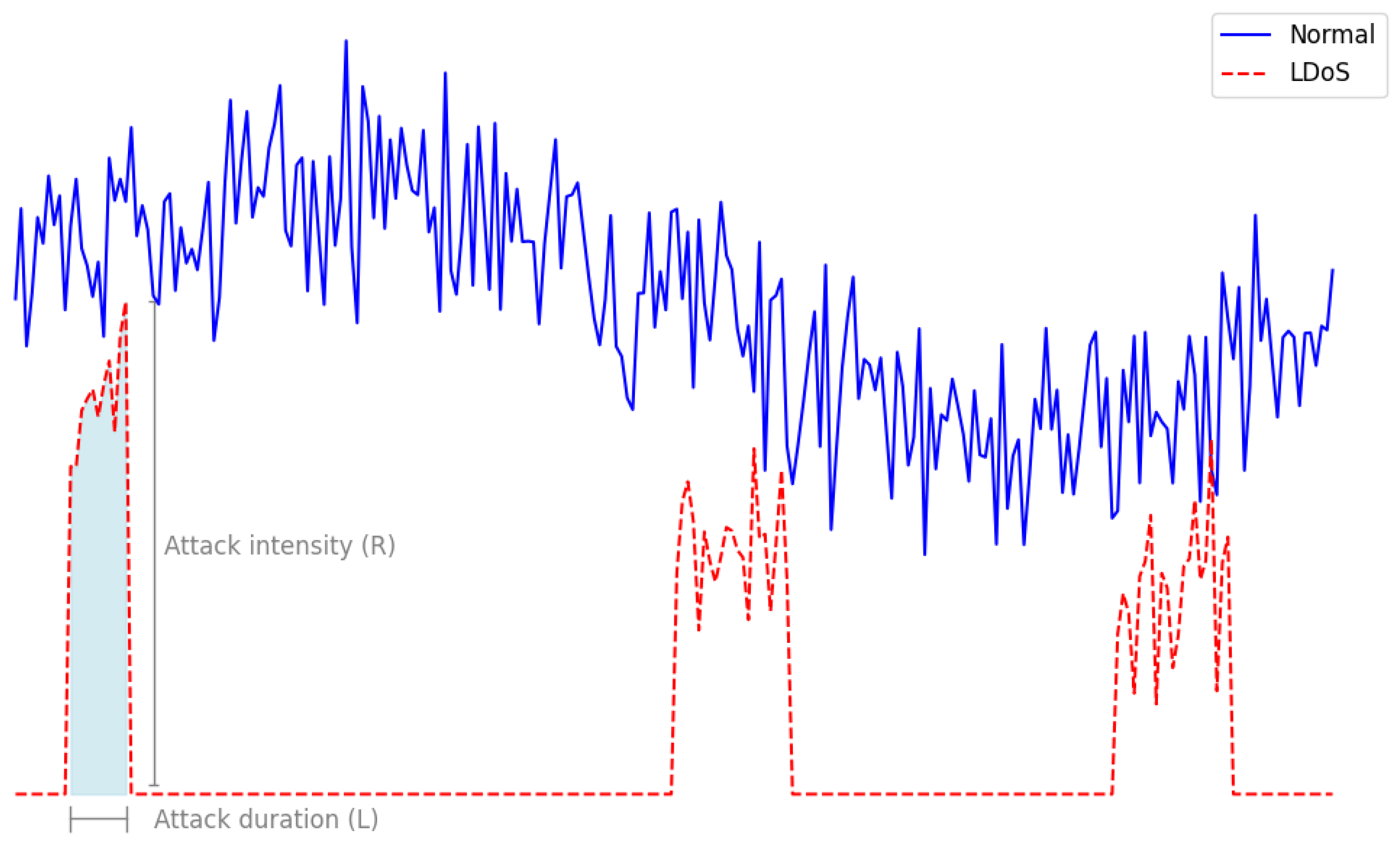
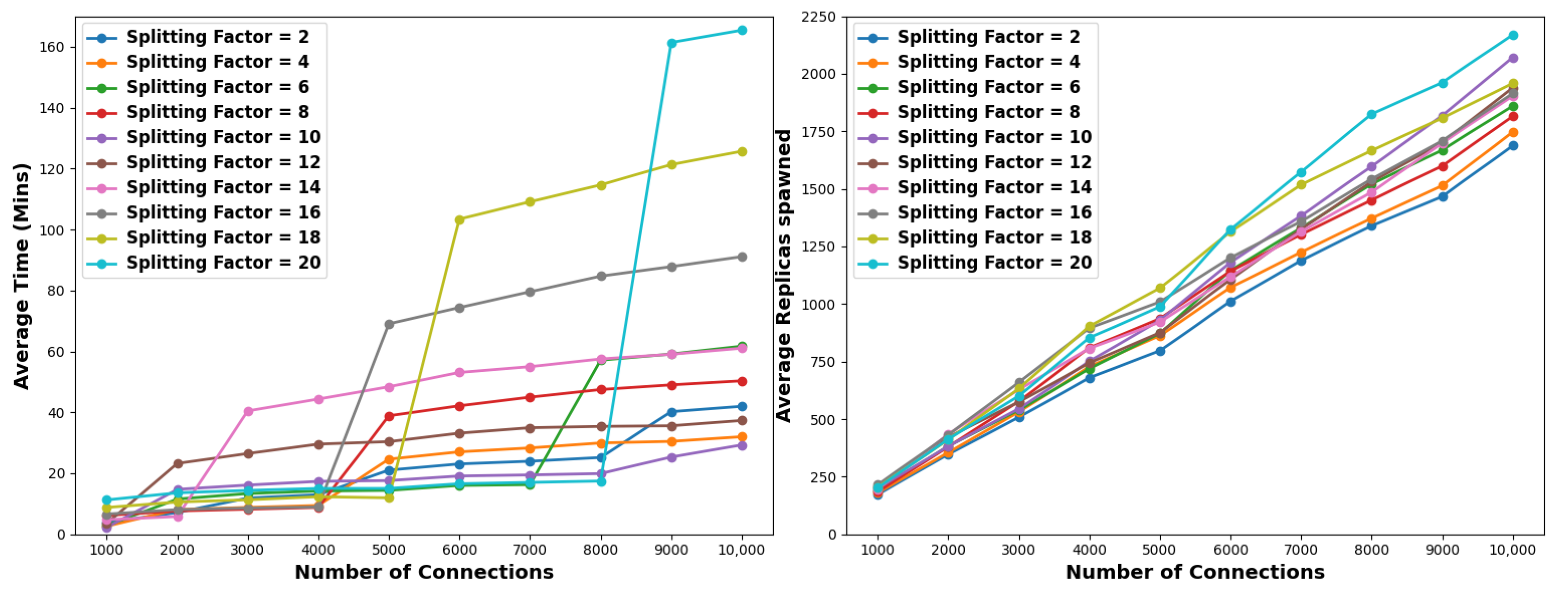
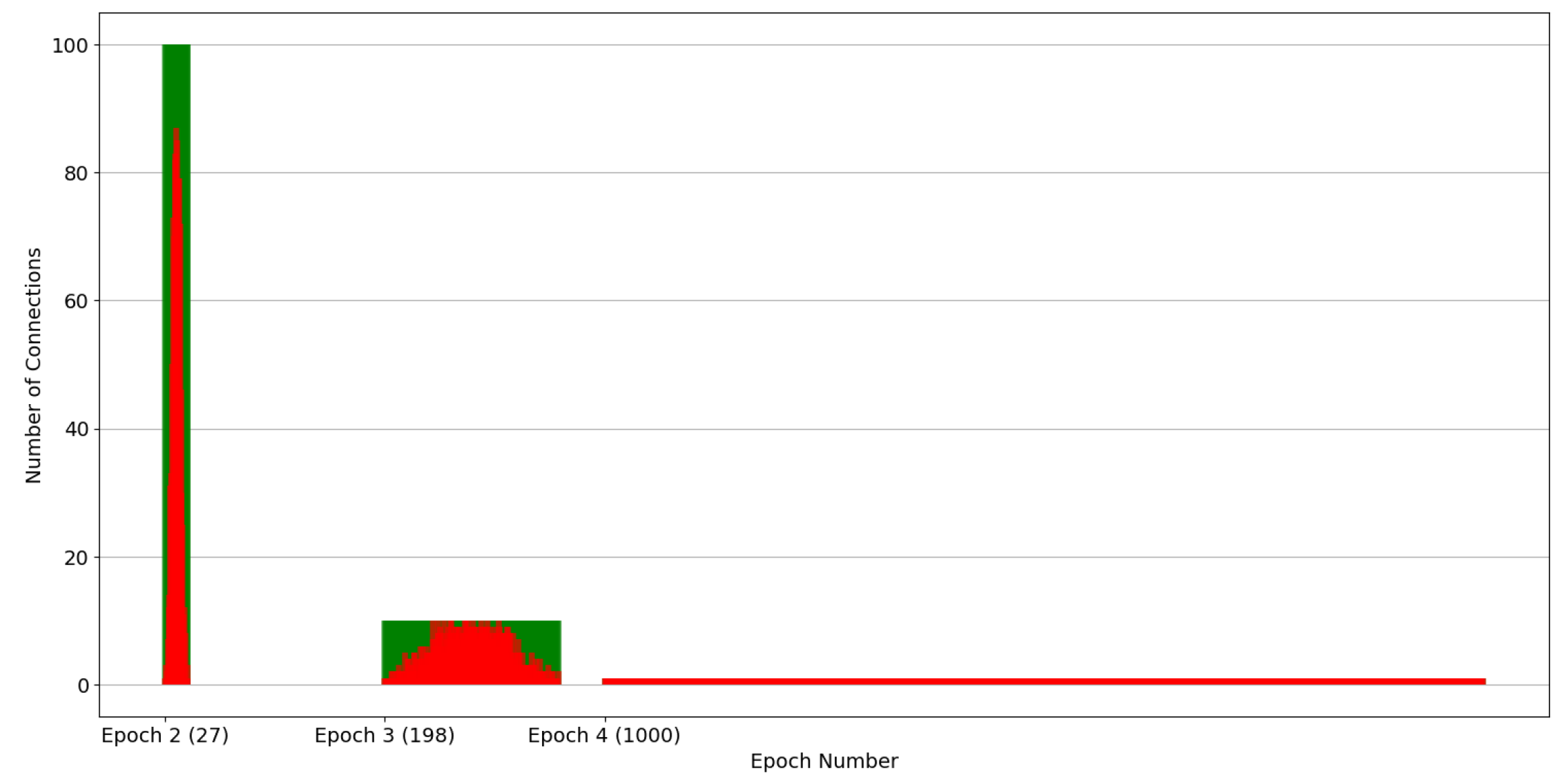
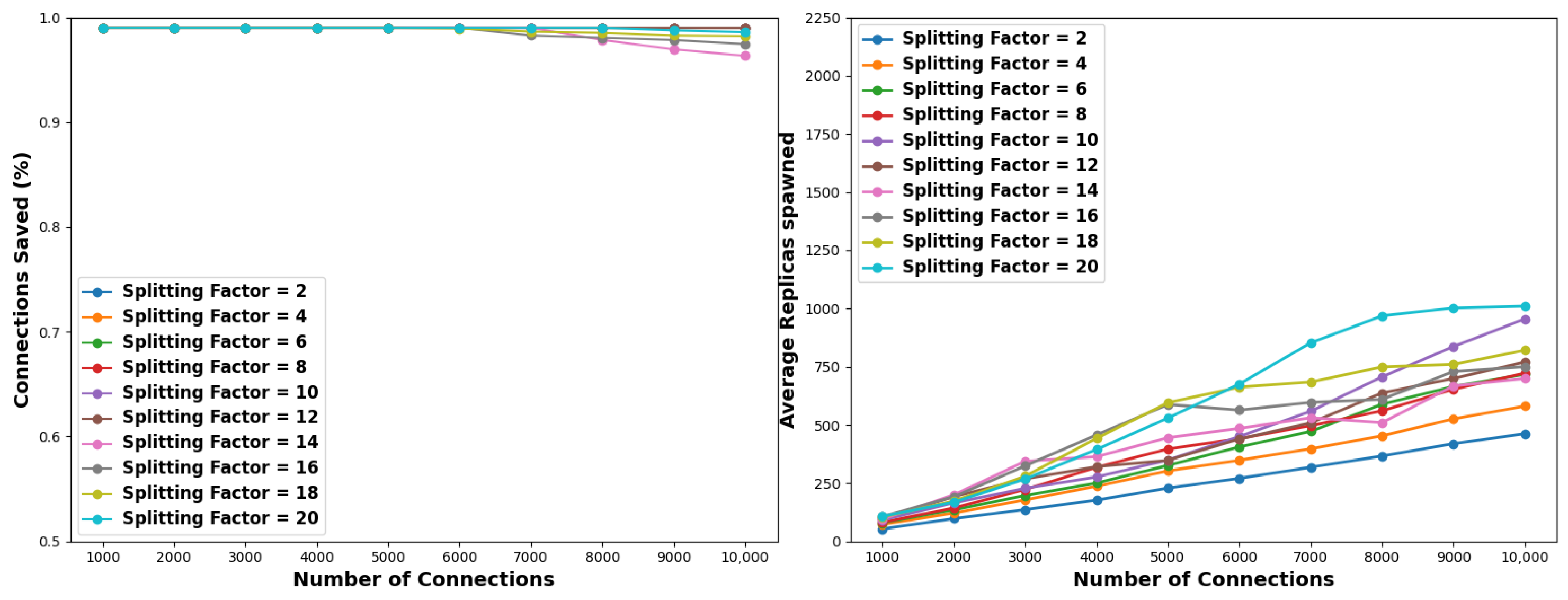
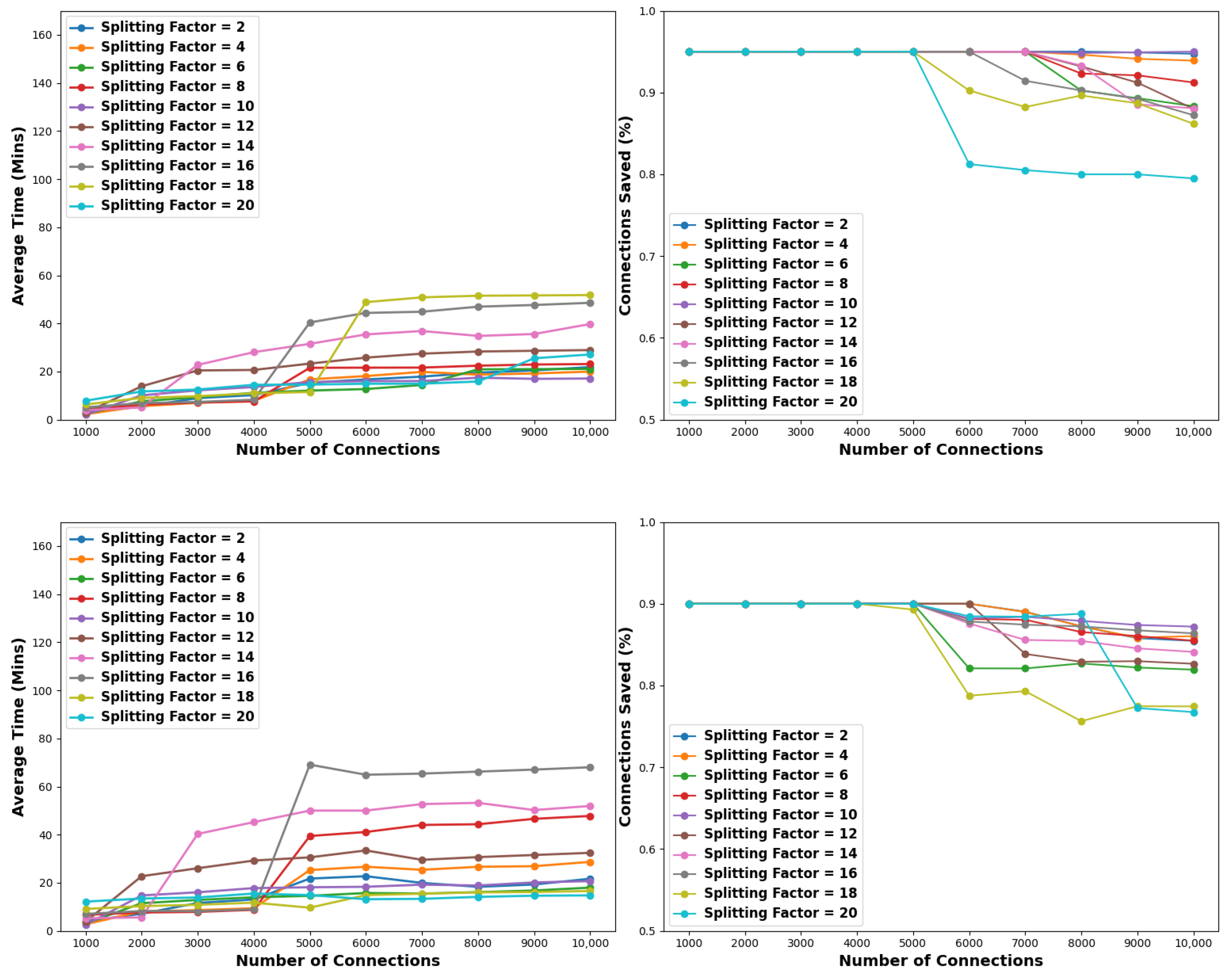
Table 1.
Average times for all the actions performed per epoch for various replica numbers and connection pools.
Table 1.
Average times for all the actions performed per epoch for various replica numbers and connection pools.
| Time (s) | |||||
|---|---|---|---|---|---|
| Replicas (r)/Connections (c) Num. | 10 | 20 | 30 | 40 | 50 |
| 5.13 | 7.77 | 10.36 | 13.75 | 18.04 | |
| 0.002 | 0.005 | 0.008 | 0.011 | 0.015 | |
| 0.006 | 0.015 | 0.021 | 0.029 | 0.033 | |
Table 2.
Time elapsed in minutes (left) and resource consumption (right).
| Time (min) | Num. of Replicas | ||||
|---|---|---|---|---|---|
| Num. of Conn. | Par. Approach | Ser. Approach | Num. of Conn. | Par. Approach | Ser. Approach |
| 1000 | 0.18 | 83.52 | 1000 | 1000 | 1 |
| 2000 | 0.27 | 167.10 | 2000 | 2000 | 1 |
| 3000 | 0.37 | 250.55 | 3000 | 3000 | 1 |
| 4000 | 0.45 | 334.12 | 4000 | 4000 | 1 |
| 5000 | 0.54 | 417.37 | 5000 | 5000 | 1 |
| 6000 | 0.64 | 501.28 | 6000 | 6000 | 1 |
| 7000 | 0.73 | 584.64 | 7000 | 7000 | 1 |
| 8000 | 0.82 | 668.07 | 8000 | 8000 | 1 |
| 9000 | 0.91 | 751.45 | 9000 | 9000 | 1 |
| 10,000 | 1.00 | 835.20 | 10,000 | 10,000 | 1 |
Table 3.
Time elapsed in minutes (top) and resource consumption (bottom) when considering a pollution factor of 1%. Highlighted are the best (green) and worst (red) configurations.
Table 3.
Time elapsed in minutes (top) and resource consumption (bottom) when considering a pollution factor of 1%. Highlighted are the best (green) and worst (red) configurations.
| Num. of connections | SF = 2 | SF = 4 | SF = 6 | SF = 8 | SF = 10 | SF = 12 | SF = 14 | SF = 16 | SF = 18 | SF = 20 |
| 1000 | 1.84 | 1.25 | 1.26 | 1.74 | 1.23 | 1.58 | 2.03 | 2.12 | 2.34 | 2.91 |
| 2000 | 2.97 | 2.62 | 2.95 | 2.73 | 3.61 | 4.34 | 2.96 | 3.46 | 3.67 | 4.38 |
| 3000 | 4.18 | 3.29 | 3.92 | 3.38 | 4.49 | 6.08 | 7.47 | 4.11 | 5.16 | 5.86 |
| 4000 | 4.82 | 3.75 | 4.61 | 3.82 | 5.53 | 6.80 | 8.64 | 4.61 | 5.72 | 7.14 |
| 5000 | 6.60 | 6.22 | 5.48 | 8.06 | 6.58 | 8.65 | 10.41 | 12.87 | 7.21 | 8.09 |
| 6000 | 6.98 | 6.62 | 5.70 | 8.92 | 6.69 | 9.16 | 11.60 | 13.95 | 16.34 | 8.53 |
| 7000 | 7.73 | 7.50 | 6.62 | 10.19 | 7.72 | 10.18 | 13.02 | 15.69 | 18.60 | 9.65 |
| 8000 | 8.32 | 7.96 | 10.72 | 10.71 | 8.09 | 10.59 | 13.72 | 16.49 | 19.13 | 9.76 |
| 9000 | 11.11 | 9.21 | 12.79 | 12.59 | 9.18 | 12.65 | 16.20 | 19.58 | 23.24 | 26.73 |
| 10,000 | 11.61 | 9.61 | 13.10 | 13.11 | 9.52 | 12.95 | 16.67 | 20.22 | 24.27 | 27.68 |
| Num. of connections | SF = 2 | SF = 4 | SF = 6 | SF = 8 | SF = 10 | SF = 12 | SF = 14 | SF = 16 | SF = 18 | SF = 20 |
| 1000 | 49 | 64 | 69 | 80 | 100 | 92 | 94 | 87 | 88 | 114 |
| 2000 | 100 | 126 | 138 | 147 | 165 | 200 | 213 | 193 | 169 | 168 |
| 3000 | 144 | 184 | 200 | 225 | 217 | 279 | 355 | 301 | 294 | 267 |
| 4000 | 179 | 238 | 254 | 309 | 283 | 287 | 389 | 428 | 403 | 403 |
| 5000 | 235 | 304 | 341 | 398 | 379 | 420 | 474 | 602 | 619 | 532 |
| 6000 | 259 | 323 | 387 | 434 | 408 | 424 | 501 | 576 | 684 | 656 |
| 7000 | 302 | 388 | 491 | 495 | 541 | 510 | 559 | 650 | 785 | 860 |
| 8000 | 338 | 412 | 521 | 515 | 610 | 534 | 568 | 645 | 797 | 970 |
| 9000 | 413 | 511 | 685 | 648 | 818 | 691 | 717 | 806 | 983 | 1040 |
| 10,000 | 440 | 542 | 675 | 662 | 901 | 737 | 740 | 802 | 945 | 1061 |
Table 4.
Time elapsed in minutes (top) and resource consumption (bottom) when considering a pollution factor of 5%. Highlighted are the best (green) and worst (red) configurations.
Table 4.
Time elapsed in minutes (top) and resource consumption (bottom) when considering a pollution factor of 5%. Highlighted are the best (green) and worst (red) configurations.
| Num. of connections | SF = 2 | SF = 4 | SF = 6 | SF = 8 | SF = 10 | SF = 12 | SF = 14 | SF = 16 | SF = 18 | SF = 20 |
| 1000 | 3.03 | 2.15 | 2.23 | 4.06 | 1.97 | 2.91 | 3.70 | 5.14 | 5.89 | 6.85 |
| 2000 | 5.31 | 5.53 | 7.26 | 5.75 | 9.28 | 13.38 | 4.87 | 6.47 | 7.99 | 9.87 |
| 3000 | 8.98 | 7.10 | 9.78 | 7.16 | 11.86 | 17.69 | 23.28 | 7.79 | 10.56 | 13.05 |
| 4000 | 10.05 | 7.71 | 10.91 | 7.46 | 14.11 | 20.35 | 27.14 | 7.89 | 10.51 | 13.48 |
| 5000 | 14.78 | 16.13 | 11.61 | 24.16 | 14.38 | 23.04 | 32.00 | 40.44 | 10.91 | 13.75 |
| 6000 | 16.48 | 18.09 | 12.79 | 26.80 | 15.51 | 24.27 | 34.86 | 46.03 | 57.21 | 15.04 |
| 7000 | 17.92 | 19.77 | 13.78 | 30.00 | 16.80 | 27.16 | 38.32 | 50.08 | 62.98 | 15.31 |
| 8000 | 19.62 | 21.78 | 35.18 | 32.83 | 18.10 | 32.31 | 41.92 | 56.09 | 68.80 | 16.26 |
| 9000 | 27.35 | 22.12 | 36.13 | 33.91 | 18.86 | 37.78 | 43.44 | 57.79 | 75.72 | 90.28 |
| 10,000 | 29.72 | 24.51 | 39.95 | 37.30 | 19.91 | 41.86 | 46.64 | 64.07 | 81.17 | 97.92 |
| Num. of connections | SF = 2 | SF = 4 | SF = 6 | SF = 8 | SF = 10 | SF = 12 | SF = 14 | SF = 16 | SF = 18 | SF = 20 |
| 1000 | 118 | 138 | 141 | 136 | 168 | 170 | 151 | 163 | 152 | 149 |
| 2000 | 233 | 258 | 291 | 288 | 279 | 353 | 360 | 342 | 313 | 296 |
| 3000 | 386 | 430 | 439 | 504 | 452 | 477 | 620 | 592 | 593 | 566 |
| 4000 | 483 | 580 | 565 | 673 | 631 | 587 | 677 | 777 | 755 | 746 |
| 5000 | 596 | 698 | 718 | 808 | 763 | 734 | 778 | 894 | 973 | 928 |
| 6000 | 720 | 808 | 911 | 932 | 959 | 880 | 890 | 1012 | 1189 | 1193 |
| 7000 | 851 | 947 | 1120 | 1045 | 1092 | 1079 | 1046 | 1113 | 1321 | 1405 |
| 8000 | 989 | 1088 | 1313 | 1202 | 1147 | 1303 | 1215 | 1303 | 1469 | 1692 |
| 9000 | 1076 | 1158 | 1349 | 1220 | 1202 | 1377 | 1314 | 1288 | 1438 | 1653 |
| 10,000 | 1245 | 1378 | 1567 | 1488 | 1364 | 1666 | 1552 | 1573 | 1641 | 1953 |
Table 5.
Time elapsed in minutes (top) and resource consumption (bottom) when considering a pollution factor of 10%. Highlighted are the best (green) and worst (red) configurations.
Table 5.
Time elapsed in minutes (top) and resource consumption (bottom) when considering a pollution factor of 10%. Highlighted are the best (green) and worst (red) configurations.
| Num. of connections | SF = 2 | SF = 4 | SF = 6 | SF = 8 | SF = 10 | SF = 12 | SF = 14 | SF = 16 | SF = 18 | SF = 20 |
| 1000 | 3.85 | 2.63 | 2.85 | 6.20 | 2.23 | 3.53 | 4.79 | 6.65 | 8.82 | 11.30 |
| 2000 | 7.17 | 8.13 | 11.58 | 7.67 | 14.76 | 23.25 | 5.84 | 8.12 | 10.61 | 13.62 |
| 3000 | 11.92 | 8.85 | 13.39 | 8.25 | 16.14 | 26.53 | 40.45 | 8.63 | 11.34 | 14.41 |
| 4000 | 13.01 | 9.48 | 14.21 | 8.84 | 17.36 | 29.62 | 44.38 | 8.99 | 12.35 | 15.05 |
| 5000 | 21.04 | 24.67 | 14.42 | 38.85 | 17.62 | 30.43 | 48.44 | 69.10 | 11.99 | 15.06 |
| 6000 | 23.08 | 27.08 | 16.03 | 42.15 | 19.11 | 33.19 | 53.10 | 74.37 | 103.45 | 16.58 |
| 7000 | 23.97 | 28.36 | 16.29 | 45.02 | 19.46 | 34.96 | 54.99 | 79.57 | 109.13 | 17.02 |
| 8000 | 25.21 | 30.00 | 57.10 | 47.52 | 19.90 | 35.38 | 57.50 | 84.73 | 114.60 | 17.47 |
| 9000 | 40.21 | 30.51 | 59.11 | 49.05 | 25.36 | 35.58 | 59.04 | 87.84 | 121.32 | 161.40 |
| 10,000 | 42.14 | 32.03 | 61.72 | 50.38 | 29.03 | 37.30 | 61.05 | 91.10 | 125.72 | 165.43 |
| Num. of connections | SF = 2 | SF = 4 | SF = 6 | SF = 8 | SF = 10 | SF = 12 | SF = 14 | SF = 16 | SF = 18 | SF = 20 |
| 1000 | 173 | 180 | 190 | 185 | 199 | 210 | 197 | 215 | 205 | 202 |
| 2000 | 348 | 356 | 384 | 381 | 383 | 422 | 435 | 432 | 412 | 414 |
| 3000 | 508 | 531 | 539 | 577 | 545 | 575 | 629 | 660 | 633 | 601 |
| 4000 | 680 | 728 | 719 | 810 | 751 | 744 | 807 | 896 | 904 | 854 |
| 5000 | 797 | 863 | 873 | 937 | 930 | 876 | 922 | 1009 | 1069 | 988 |
| 6000 | 1012 | 1072 | 1146 | 1143 | 1181 | 1107 | 1119 | 1201 | 1314 | 1324 |
| 7000 | 1189 | 1225 | 1331 | 1302 | 1384 | 1326 | 1315 | 1359 | 1518 | 1574 |
| 8000 | 1340 | 1373 | 1521 | 1452 | 1598 | 1531 | 1486 | 1543 | 1667 | 1825 |
| 9000 | 1467 | 1514 | 1669 | 1600 | 1818 | 1700 | 1699 | 1709 | 1807 | 1962 |
| 10,000 | 1688 | 1747 | 1860 | 1815 | 2071 | 1940 | 1904 | 1915 | 1959 | 2170 |
Table 6.
Average connections saved and time elapsed per epoch for partitioning factor 2.
| Partitioning Factor | Average Connections Saved (%) | Average Time Elapsed (m) |
|---|---|---|
| Epoch 1 | 0 | 1.01 |
| Epoch 2 | 50 | 1.59 |
| Epoch 3 | 50 | 1.93 |
| Epoch 4 | 62.50 | 2.20 |
| Epoch 5 | 68.75 | 2.44 |
| Epoch 6 | 71.87 | 2.72 |
| Epoch 7 | 74.21 | 3.13 |
| Epoch 8 | 75.38 | 3.79 |
| Epoch 9 | 77.72 | 4.95 |
| Epoch 10 | 79.96 | 6.98 |
| Epoch 11 | 82.75 | 10.56 |
| Epoch 12 | 85.65 | 16.89 |
| Epoch 13 | 88.73 | 26.93 |
| Epoch 14 | 90 | 42.14 |
Table 7.
Average connections saved and time elapsed per epoch for partitioning factor 10.
| Partitioning Factor | Average Connections Saved (%) | Average Time Elapsed (m) |
|---|---|---|
| Epoch 1 | 60 | 1.08 |
| Epoch 2 | 73 | 1.59 |
| Epoch 3 | 80.20 | 3.99 |
| Epoch 4 | 90 | 29.04 |
Table 8.
Detection rate (top) and resources consumption (bottom) when considering a pollution factor of 1%. Highlighted are the worst (red) configurations. Empty cells indicate that all benign connections (99% of all connections) were saved
Table 8.
Detection rate (top) and resources consumption (bottom) when considering a pollution factor of 1%. Highlighted are the worst (red) configurations. Empty cells indicate that all benign connections (99% of all connections) were saved
| Num. of connections | SF = 2 | SF = 4 | SF = 6 | SF = 8 | SF = 10 | SF = 12 | SF = 14 | SF = 16 | SF = 18 | SF = 20 |
| 1000 | ||||||||||
| 2000 | ||||||||||
| 3000 | ||||||||||
| 4000 | ||||||||||
| 5000 | ||||||||||
| 6000 | 98.9 | |||||||||
| 7000 | 98.2 | 98.6 | ||||||||
| 8000 | 97.8 | 98.0 | 98.5 | |||||||
| 9000 | 96.9 | 97.8 | 98.2 | 98.7 | ||||||
| 10,000 | 96.3 | 97.4 | 98.2 | 98.5 | ||||||
| Num. of connections | SF = 2 | SF = 4 | SF = 6 | SF = 8 | SF = 10 | SF = 12 | SF = 14 | SF = 16 | SF = 18 | SF = 20 |
| 1000 | ||||||||||
| 2000 | ||||||||||
| 3000 | ||||||||||
| 4000 | ||||||||||
| 5000 | ||||||||||
| 6000 | 662 | |||||||||
| 7000 | 597 | 684 | ||||||||
| 8000 | 510 | 610 | 749 | |||||||
| 9000 | 667 | 729 | 760 | 1002 | ||||||
| 10,000 | 699 | 750 | 821 | 1010 |
Table 9.
Detection rate (top) and resources consumption (bottom) when considering a pollution factor of 5%. Highlighted are the best (green) and worst (red) configurations. Empty cells indicate that all benign connections (95% of all connections) were saved.
Table 9.
Detection rate (top) and resources consumption (bottom) when considering a pollution factor of 5%. Highlighted are the best (green) and worst (red) configurations. Empty cells indicate that all benign connections (95% of all connections) were saved.
| Num. of connections | SF = 2 | SF = 4 | SF = 6 | SF = 8 | SF = 10 | SF = 12 | SF = 14 | SF = 16 | SF = 18 | SF = 20 |
| 1000 | ||||||||||
| 2000 | 89.3 | |||||||||
| 3000 | 90.9 | 94.4 | ||||||||
| 4000 | 90.6 | 92.7 | ||||||||
| 5000 | 94.7 | 88.6 | 88.9 | 91.6 | 88.2 | |||||
| 6000 | 94.7 | 93.8 | 88.9 | 88.4 | 90.8 | 87.6 | 89.8 | |||
| 7000 | 94.3 | 92.4 | 87.5 | 94.8 | 87.7 | 90.4 | 85.2 | 84.1 | ||
| 8000 | 93.6 | 91.9 | 89.7 | 87.2 | 94.5 | 86.9 | 89.4 | 84.2 | 83.2 | |
| 9000 | 90.7 | 90.8 | 88.3 | 87.7 | 94.7 | 85.9 | 88.2 | 83.8 | 83.5 | 82.2 |
| 10,000 | 89.8 | 89.9 | 86 | 87.4 | 94.4 | 85 | 87.8 | 83.2 | 82 | 81.3 |
| Num. of connections | SF = 2 | SF = 4 | SF = 6 | SF = 8 | SF = 10 | SF = 12 | SF = 14 | SF = 16 | SF = 18 | SF = 20 |
| 1000 | ||||||||||
| 2000 | 386 | |||||||||
| 3000 | 404 | 516 | ||||||||
| 4000 | 543 | 624 | ||||||||
| 5000 | 615 | 730 | 621 | 710 | 824 | |||||
| 6000 | 659 | 711 | 833 | 719 | 764 | 852 | 965 | |||
| 7000 | 721 | 823 | 884 | 857 | 726 | 785 | 870 | 936 | ||
| 8000 | 728 | 863 | 945 | 825 | 899 | 753 | 795 | 824 | 978 | |
| 9000 | 757 | 834 | 964 | 853 | 917 | 719 | 775 | 910 | 943 | 1084 |
| 10,000 | 784 | 879 | 928 | 876 | 928 | 769 | 787 | 852 | 982 | 1090 |
Table 10.
Detection rate (top) and resources consumption (bottom) when considering a pollution factor of 10%. Highlighted are the best (green) and worst (red) configurations. Empty cells indicate that all benign connections (90% of all connections) were saved.
Table 10.
Detection rate (top) and resources consumption (bottom) when considering a pollution factor of 10%. Highlighted are the best (green) and worst (red) configurations. Empty cells indicate that all benign connections (90% of all connections) were saved.
| Num. of connections | SF = 2 | SF = 4 | SF = 6 | SF = 8 | SF = 10 | SF = 12 | SF = 14 | SF = 16 | SF = 18 | SF = 20 |
| 1000 | ||||||||||
| 2000 | 89.3 | |||||||||
| 3000 | 89.5 | 87.3 | 89.4 | |||||||
| 4000 | 88.8 | 86 | 88 | |||||||
| 5000 | 88.8 | 88.8 | 88.9 | 87.6 | 85.1 | 86.8 | 87.7 | |||
| 6000 | 86.3 | 87.6 | 81.9 | 87.5 | 87.9 | 83.2 | 85.6 | 86.5 | 84.3 | 89.3 |
| 7000 | 85.2 | 87.2 | 82 | 87.2 | 87.8 | 83.3 | 85.3 | 86.2 | 83 | 88.9 |
| 8000 | 83.6 | 86.5 | 82 | 86.4 | 86.9 | 83.1 | 84.9 | 86.6 | 83.1 | 88.9 |
| 9000 | 83.4 | 86.2 | 81.6 | 86 | 86.4 | 82.7 | 84.3 | 85.9 | 83.7 | 77.7 |
| 10,000 | 82.5 | 85.4 | 80.9 | 85.4 | 86.1 | 81.8 | 83.9 | 85.4 | 84.9 | 77 |
| Num. of connections | SF = 2 | SF = 4 | SF = 6 | SF = 8 | SF = 10 | SF = 12 | SF = 14 | SF = 16 | SF = 18 | SF = 20 |
| 1000 | ||||||||||
| 2000 | 386 | |||||||||
| 3000 | 460 | 498 | 569 | |||||||
| 4000 | 578 | 673 | 727 | |||||||
| 5000 | 710 | 766 | 910 | 601 | 725 | 802 | 936 | |||
| 6000 | 755 | 813 | 878 | 953 | 790 | 671 | 832 | 955 | 1000 | 1166 |
| 7000 | 824 | 815 | 842 | 991 | 780 | 721 | 908 | 975 | 1094 | 1186 |
| 8000 | 774 | 974 | 886 | 982 | 810 | 807 | 871 | 980 | 1070 | 1106 |
| 9000 | 780 | 823 | 891 | 993 | 832 | 831 | 887 | 979 | 1081 | 1144 |
| 10,000 | 813 | 789 | 861 | 962 | 876 | 862 | 856 | 973 | 1095 | 1182 |
Table 11.
Time elapsed in minutes (top) and detection rate (bottom) when considering a pollution factor of 5%. Highlighted are the best (green) and worst (red) configurations. Note that empty cells indicate that all benign connections (95% of all connections) were saved.
Table 11.
Time elapsed in minutes (top) and detection rate (bottom) when considering a pollution factor of 5%. Highlighted are the best (green) and worst (red) configurations. Note that empty cells indicate that all benign connections (95% of all connections) were saved.
| Num. of connections | SF = 2 | SF = 4 | SF = 6 | SF = 8 | SF = 10 | SF = 12 | SF = 14 | SF = 16 | SF = 18 | SF = 20 |
| 1000 | ||||||||||
| 2000 | ||||||||||
| 3000 | ||||||||||
| 4000 | ||||||||||
| 5000 | ||||||||||
| 6000 | 48.86 | 14.94 | ||||||||
| 7000 | 44.88 | 50.86 | 14.98 | |||||||
| 8000 | 18.74 | 20.94 | 22.46 | 17.48 | 28.34 | 34.84 | 46.98 | 51.53 | 15.88 | |
| 9000 | 20.48 | 19.23 | 21.03 | 22.95 | 16.99 | 28.65 | 35.62 | 47.68 | 51.66 | 25.54 |
| 10,000 | 21.88 | 19.99 | 21.13 | 23.15 | 17.13 | 28.95 | 39.77 | 48.59 | 51.80 | 27.12 |
| Num. of connections | SF = 2 | SF = 4 | SF = 6 | SF = 8 | SF = 10 | SF = 12 | SF = 14 | SF = 16 | SF = 18 | SF = 20 |
| 1000 | ||||||||||
| 2000 | ||||||||||
| 3000 | ||||||||||
| 4000 | ||||||||||
| 5000 | ||||||||||
| 6000 | 90.2 | 81.2 | ||||||||
| 7000 | 91.4 | 88.2 | 80.5 | |||||||
| 8000 | 94.6 | 90.2 | 92.3 | 94.8 | 93.1 | 93.2 | 90.2 | 89.6 | 80 | |
| 9000 | 94.8 | 94.1 | 89.3 | 92 | 94.9 | 91.2 | 88.5 | 89.2 | 88.6 | 80 |
| 10,000 | 94.7 | 93.8 | 88.3 | 91.2 | 94.9 | 88 | 88 | 87.2 | 86.1 | 79.5 |
Table 12.
Time elapsed in minutes (top) and detection rate (bottom) when considering a pollution factor of 10%. Highlighted are the best (green) and worst (red) configurations. Note that empty cells indicate that all benign connections (90% of all connections) were saved.
Table 12.
Time elapsed in minutes (top) and detection rate (bottom) when considering a pollution factor of 10%. Highlighted are the best (green) and worst (red) configurations. Note that empty cells indicate that all benign connections (90% of all connections) were saved.
| Num. of connections | SF = 2 | SF = 4 | SF = 6 | SF = 8 | SF = 10 | SF = 12 | SF = 14 | SF = 16 | SF = 18 | SF = 20 |
| 1000 | ||||||||||
| 2000 | ||||||||||
| 3000 | ||||||||||
| 4000 | ||||||||||
| 5000 | 9.65 | |||||||||
| 6000 | 15.75 | 41.12 | 18.34 | 50.01 | 64.91 | 14.89 | 13.18 | |||
| 7000 | 19.95 | 25.41 | 15.53 | 44.05 | 19.22 | 29.55 | 52.71 | 65.39 | 15.47 | 13.80 |
| 8000 | 18.32 | 26.65 | 16.12 | 44.33 | 18.80 | 30.68 | 53.23 | 66.20 | 16.03 | 14.15 |
| 9000 | 19.29 | 26.90 | 16.79 | 46.58 | 20.15 | 31.55 | 50.23 | 67.05 | 16.18 | 14.63 |
| 10,000 | 21.69 | 28.70 | 17.98 | 47.78 | 20.70 | 32.45 | 51.93 | 68.01 | 16.59 | 14.77 |
| Num. of connections | SF = 2 | SF = 4 | SF = 6 | SF = 8 | SF = 10 | SF = 12 | SF = 14 | SF = 16 | SF = 18 | SF = 20 |
| 1000 | ||||||||||
| 2000 | ||||||||||
| 3000 | ||||||||||
| 4000 | ||||||||||
| 5000 | 89.2 | |||||||||
| 6000 | 82.1 | 88.1 | 88.2 | 87.5 | 87.8 | 78.7 | 88.4 | |||
| 7000 | 89 | 88.9 | 82 | 88 | 88.4 | 83.8 | 85.5 | 87.4 | 79.3 | 88.4 |
| 8000 | 87.2 | 87.2 | 82.7 | 86.5 | 87.9 | 82.9 | 85.4 | 87.2 | 75.6 | 88.7 |
| 9000 | 85.7 | 85.8 | 82.2 | 86 | 87.4 | 82.9 | 84.5 | 86.7 | 77.4 | 77.2 |
| 10,000 | 85.4 | 86 | 81.9 | 85.4 | 87.2 | 82.6 | 84.1 | 86.3 | 77.4 | 76.7 |
Table 13.
Time elapsed in minutes (top) and resources consumption (bottom) when considering a pollution factor of 1%. Highlighted are the best (green) and worst (red) configurations.
Table 13.
Time elapsed in minutes (top) and resources consumption (bottom) when considering a pollution factor of 1%. Highlighted are the best (green) and worst (red) configurations.
| Num. of connections | SF = 2 | SF = 4 | SF = 6 | SF = 8 | SF = 10 | SF = 12 | SF = 14 | SF = 16 | SF = 18 | SF = 20 |
| 1000 | 0.62 | 0.38 | 0.42 | 0.47 | 0.52 | 0.27 | 0.29 | 0.31 | 0.32 | 0.34 |
| 2000 | 0.79 | 0.49 | 0.53 | 0.57 | 0.62 | 0.77 | 0.84 | 0.40 | 0.42 | 1.21 |
| 3000 | 1.13 | 0.85 | 0.64 | 0.68 | 0.72 | 0.87 | 1.06 | 1.14 | 1.22 | 1.31 |
| 4000 | 1.53 | 0.97 | 0.74 | 0.78 | 0.90 | 0.97 | 1.15 | 1.23 | 1.32 | 1.58 |
| 5000 | 2.03 | 1.62 | 1.35 | 1.87 | 1.09 | 1.17 | 1.25 | 1.33 | 1.41 | 1.84 |
| 6000 | 2.23 | 1.77 | 1.47 | 2.04 | 1.20 | 1.27 | 1.35 | 1.43 | 1.66 | 1.94 |
| 7000 | 2.42 | 1.90 | 1.58 | 2.14 | 1.21 | 1.37 | 1.45 | 1.53 | 1.77 | 2.03 |
| 8000 | 2.56 | 1.99 | 1.64 | 2.18 | 1.22 | 1.37 | 1.55 | 1.63 | 1.86 | 2.15 |
| 9000 | 2.74 | 2.10 | 1.80 | 2.28 | 1.41 | 1.47 | 1.65 | 1.72 | 1.96 | 2.26 |
| 10,000 | 2.93 | 2.23 | 1.89 | 2.39 | 1.42 | 1.57 | 1.74 | 1.82 | 2.00 | 2.42 |
| Num. of connections | SF = 2 | SF = 4 | SF = 6 | SF = 8 | SF = 10 | SF = 12 | SF = 14 | SF = 16 | SF = 18 | SF = 20 |
| 1000 | 8 | 10 | 16 | 22 | 28 | 12 | 14 | 16 | 18 | 20 |
| 2000 | 8 | 10 | 16 | 22 | 28 | 45 | 53 | 16 | 18 | 96 |
| 3000 | 12 | 22 | 16 | 22 | 28 | 45 | 66 | 76 | 86 | 96 |
| 4000 | 19 | 22 | 16 | 22 | 37 | 45 | 66 | 76 | 86 | 115 |
| 5000 | 33 | 61 | 56 | 113 | 46 | 56 | 66 | 76 | 86 | 134 |
| 6000 | 34 | 64 | 56 | 120 | 46 | 56 | 66 | 76 | 103 | 134 |
| 7000 | 34 | 64 | 56 | 120 | 37 | 56 | 66 | 76 | 103 | 134 |
| 8000 | 32 | 61 | 56 | 113 | 28 | 45 | 66 | 76 | 103 | 134 |
| 9000 | 32 | 61 | 56 | 113 | 37 | 45 | 66 | 76 | 103 | 134 |
| 10,000 | 32 | 61 | 56 | 113 | 28 | 45 | 66 | 76 | 103 | 134 |
Table 14.
Time elapsed in minutes (top) and resources consumption (bottom) when considering a pollution factor of 5%. Highlighted are the best (green) and worst (red) configurations.
Table 14.
Time elapsed in minutes (top) and resources consumption (bottom) when considering a pollution factor of 5%. Highlighted are the best (green) and worst (red) configurations.
| Num. of connections | SF = 2 | SF = 4 | SF = 6 | SF = 8 | SF = 10 | SF = 12 | SF = 14 | SF = 16 | SF = 18 | SF = 20 |
| 1000 | 0.78 | 0.61 | 0.92 | 0.47 | 0.60 | 0.77 | 0.86 | 0.94 | 1.18 | 1.29 |
| 2000 | 1.16 | 0.72 | 1.03 | 0.58 | 0.71 | 0.88 | 0.96 | 1.04 | 1.29 | 1.39 |
| 3000 | 1.66 | 1.38 | 1.14 | 1.65 | 2.61 | 0.98 | 1.06 | 1.14 | 1.23 | 1.48 |
| 4000 | 3.57 | 3.57 | 3.91 | 2.10 | 3.22 | 4.65 | 6.40 | 3.69 | 1.62 | 1.74 |
| 5000 | 3.70 | 3.63 | 3.91 | 2.14 | 3.15 | 4.54 | 6.49 | 3.99 | 1.74 | 1.84 |
| 6000 | 3.94 | 3.78 | 4.14 | 2.04 | 3.00 | 4.64 | 6.50 | 4.02 | 1.76 | 1.77 |
| 7000 | 4.10 | 3.90 | 4.04 | 2.42 | 3.44 | 4.74 | 6.45 | 5.55 | 1.77 | 2.04 |
| 8000 | 4.50 | 4.35 | 4.45 | 2.59 | 3.72 | 5.25 | 7.27 | 5.34 | 1.88 | 2.21 |
| 9000 | 4.57 | 4.29 | 4.39 | 2.62 | 3.73 | 5.15 | 7.14 | 6.02 | 2.04 | 2.40 |
| 10,000 | 4.59 | 4.24 | 4.41 | 2.89 | 3.66 | 5.28 | 7.11 | 5.98 | 2.48 | 2.61 |
| Num. of connections | SF = 2 | SF = 4 | SF = 6 | SF = 8 | SF = 10 | SF = 12 | SF = 14 | SF = 16 | SF = 18 | SF = 20 |
| 1000 | 12 | 22 | 56 | 22 | 37 | 56 | 66 | 76 | 103 | 115 |
| 2000 | 19 | 22 | 56 | 22 | 37 | 56 | 66 | 76 | 103 | 115 |
| 3000 | 32 | 61 | 56 | 113 | 217 | 56 | 66 | 76 | 86 | 115 |
| 4000 | 123 | 235 | 306 | 148 | 271 | 430 | 625 | 217 | 120 | 134 |
| 5000 | 120 | 229 | 296 | 141 | 253 | 408 | 625 | 428 | 103 | 134 |
| 6000 | 122 | 229 | 296 | 120 | 226 | 408 | 625 | 428 | 103 | 115 |
| 7000 | 122 | 232 | 286 | 148 | 262 | 408 | 599 | 408 | 103 | 134 |
| 8000 | 135 | 259 | 316 | 155 | 280 | 452 | 677 | 510 | 120 | 134 |
| 9000 | 128 | 244 | 301 | 148 | 271 | 430 | 651 | 510 | 120 | 134 |
| 10,000 | 128 | 229 | 291 | 134 | 253 | 452 | 638 | 510 | 120 | 134 |
Table 15.
Time elapsed in minutes (top) and resources consumption (bottom) when considering a pollution factor of 10%. Highlighted are the best (green) and worst (red) configurations.
Table 15.
Time elapsed in minutes (top) and resources consumption (bottom) when considering a pollution factor of 10%. Highlighted are the best (green) and worst (red) configurations.
| Num. of connections | SF = 2 | SF = 4 | SF = 6 | SF = 8 | SF = 10 | SF = 12 | SF = 14 | SF = 16 | SF = 18 | SF = 20 |
| 1000 | 1.29 | 1.14 | 0.92 | 1.45 | 0.61 | 0.77 | 0.86 | 0.94 | 1.03 | 1.28 |
| 2000 | 2.12 | 1.37 | 1.08 | 1.75 | 2.85 | 4.15 | 5.96 | 1.04 | 1.28 | 1.55 |
| 3000 | 2.35 | 1.52 | 3.64 | 1.92 | 3.03 | 4.35 | 6.07 | 8.63 | 1.53 | 1.65 |
| 4000 | 3.60 | 3.65 | 3.86 | 2.10 | 3.23 | 4.56 | 6.40 | 9.00 | 12.05 | 15.51 |
| 5000 | 3.69 | 3.66 | 3.91 | 2.00 | 3.24 | 4.65 | 6.62 | 8.95 | 11.98 | 16.83 |
| 6000 | 6.02 | 4.05 | 4.27 | 9.74 | 3.43 | 5.07 | 7.08 | 9.88 | 13.02 | 17.27 |
| 7000 | 6.25 | 4.18 | 4.55 | 10.11 | 3.70 | 5.26 | 7.53 | 9.98 | 13.56 | 17.38 |
| 8000 | 6.50 | 4.33 | 4.59 | 10.29 | 3.80 | 5.36 | 7.62 | 10.07 | 13.81 | 17.65 |
| 9000 | 10.54 | 11.79 | 4.86 | 10.94 | 3.87 | 5.56 | 7.85 | 10.72 | 14.38 | 17.90 |
| 10,000 | 10.51 | 11.72 | 4.77 | 10.63 | 3.97 | 5.56 | 7.58 | 10.40 | 13.70 | 18.00 |
| Num. of connections | SF = 2 | SF = 4 | SF = 6 | SF = 8 | SF = 10 | SF = 12 | SF = 14 | SF = 16 | SF = 18 | SF = 20 |
| 1000 | 32 | 61 | 56 | 113 | 37 | 56 | 66 | 76 | 86 | 115 |
| 2000 | 65 | 70 | 61 | 134 | 253 | 397 | 444 | 76 | 103 | 134 |
| 3000 | 67 | 73 | 291 | 141 | 262 | 408 | 599 | 659 | 120 | 134 |
| 4000 | 125 | 241 | 301 | 148 | 271 | 419 | 625 | 895 | 881 | 854 |
| 5000 | 119 | 232 | 296 | 127 | 262 | 419 | 638 | 901 | 1070 | 1304 |
| 6000 | 240 | 256 | 321 | 897 | 271 | 452 | 677 | 991 | 1344 | 1380 |
| 7000 | 243 | 256 | 336 | 925 | 289 | 463 | 716 | 991 | 1395 | 1606 |
| 8000 | 246 | 259 | 331 | 932 | 289 | 463 | 716 | 991 | 1412 | 1844 |
| 9000 | 366 | 892 | 346 | 988 | 289 | 474 | 729 | 1051 | 1463 | 1863 |
| 10,000 | 354 | 877 | 326 | 946 | 289 | 463 | 690 | 1006 | 1378 | 1863 |
Disclaimer/Publisher’s Note: The statements, opinions and data contained in all publications are solely those of the individual author(s) and contributor(s) and not of MDPI and/or the editor(s). MDPI and/or the editor(s) disclaim responsibility for any injury to people or property resulting from any ideas, methods, instructions or products referred to in the content. |
© 2024 by the authors. Licensee MDPI, Basel, Switzerland. This article is an open access article distributed under the terms and conditions of the Creative Commons Attribution (CC BY) license (https://creativecommons.org/licenses/by/4.0/).
Share and Cite
MDPI and ACS Style
Kampourakis, V.; Makrakis, G.M.; Kolias, C. From Seek-and-Destroy to Split-and-Destroy: Connection Partitioning as an Effective Tool against Low-Rate DoS Attacks. Future Internet 2024, 16, 137. https://doi.org/10.3390/fi16040137
AMA Style
Kampourakis V, Makrakis GM, Kolias C. From Seek-and-Destroy to Split-and-Destroy: Connection Partitioning as an Effective Tool against Low-Rate DoS Attacks. Future Internet. 2024; 16(4):137. https://doi.org/10.3390/fi16040137
Chicago/Turabian StyleKampourakis, Vyron, Georgios Michail Makrakis, and Constantinos Kolias. 2024. "From Seek-and-Destroy to Split-and-Destroy: Connection Partitioning as an Effective Tool against Low-Rate DoS Attacks" Future Internet 16, no. 4: 137. https://doi.org/10.3390/fi16040137
Note that from the first issue of 2016, this journal uses article numbers instead of page numbers. See further details here.