
A Review on Hot-IP Finding Methods and Its Application in Early DDoS Target Detection


Abstract
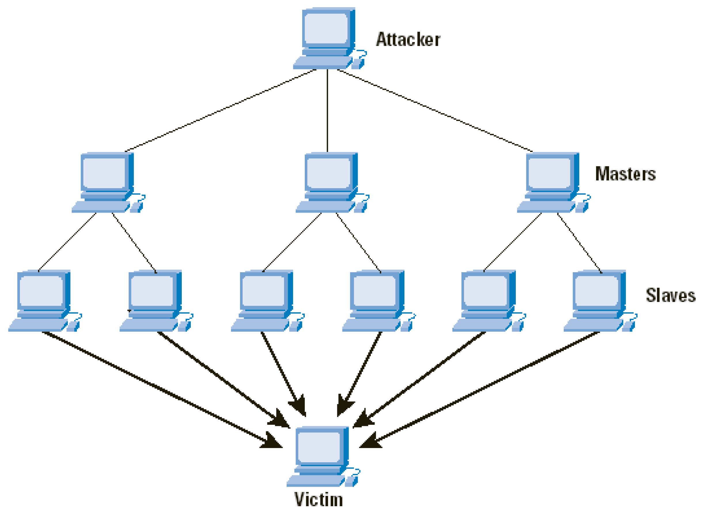
:1. Introduction
2. Hot-IP Finding Methods
2.1. Methods for Finding High-Occurrence-Frequency Elements
2.1.1. Majority
2.1.2. Frequent
2.1.3. Lossy Counting
2.1.4. Space Saving
2.1.5. Count-Sketch
2.1.6. Count-Min
2.1.7. Group Testing
2.2. Application in Finding Hot-IPs
2.2.1. Experimental Data Sets and Parameters
2.2.2. Experimental Results
2.3. Comparison of Hot-IP Finding Methods
2.3.1. Complexity of Algorithms
Count-Sketch
Count-Min
Group Testing
2.3.2. Comparison of Hot-IP Finding Time
- Scenario 1: Compare Count-Sketch and Count-Min using the same initialization parameters ε = 0.005 and δ = 0.00000001. The experiment result is shown in Table 4.
- Scenario 2: Compare Count-Sketch and Count-Min using the same processing space. For Count-Sketch, select ε = 0.01 and δ = 0.00005, and select ε = 0.00009 and δ = 0.00001 for Count-Min. The experiment result is shown in Table 5.
- Scenario 3: Compare Count-Min and Group Testing using the same matrix size. For Count-Min, select ε = 0.00045 and δ = 0.00000001, and we have the counter matrix CM[19,6041]. For Group Testing, select RS[15,3]16 and d-disjunct as 6000 (corresponding to 6000 unique IPs), and we have d-disjunct matrix m[240,6000]. The experiment result is shown in Table 6.
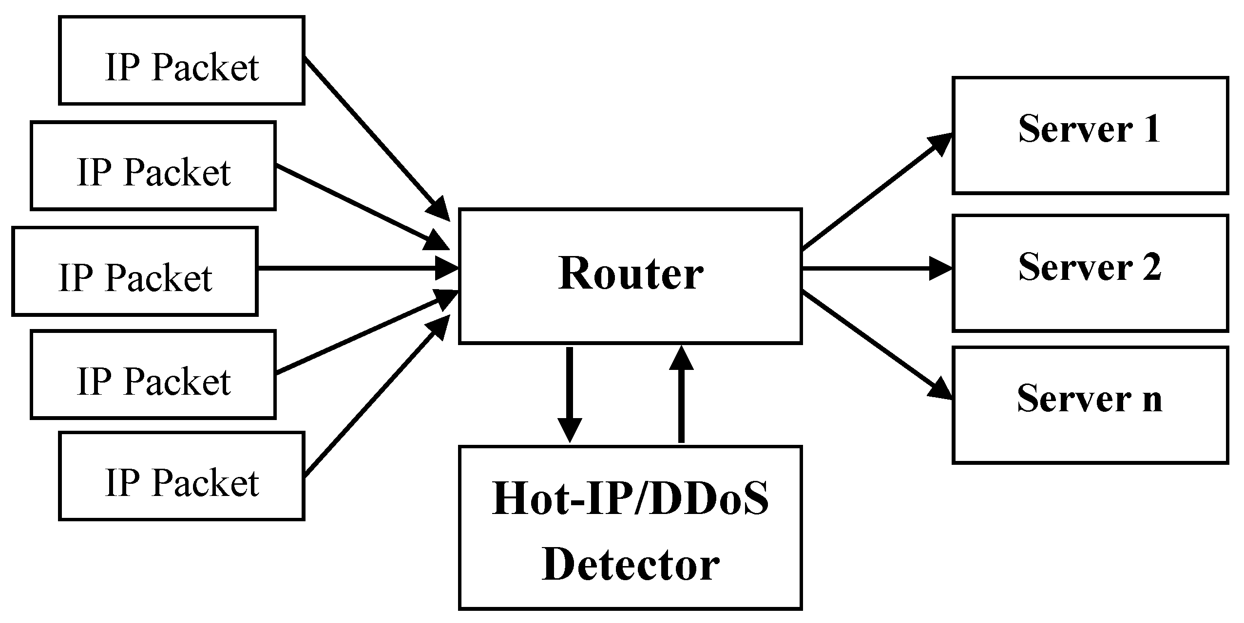
3. Proposed Target Detection Model of DDoS Attacks
4. Conclusions
Acknowledgments
Author Contributions
Conflicts of Interest
References
- Huynh, N.C.; Nguyen, D.T.; Tan, H. Finding Hot-IPs in network using Group Testing method—A review. In Proceedings of the 2012 International Conference on Green Technology and Sustainable Development (GTSD2012), Ho Chi Minh City, Vietnam, 29–30 September 2012.
- Huynh, N.C.; Nguyen, D.T.; Tan, H. Fast detection of DDoS attacks using Non-Adaptive Group Testing. Int. J. Netw. Secur. Appl. 2013, 5. [Google Scholar] [CrossRef]
- Simkhada, K.; Taleb, T.; Waizumi, Y.; Jamalipour, A.; Namoto, Y. Combating against internet worms in large-scale networks: An autonomic signature-based solution. Secur. Commun. Netw. 2009, 2, 11–78. [Google Scholar] [CrossRef]
- Boyer, B.; Moore, J. A Fast Majority Vote Algorithm; Technical Report 35; Institute for Computer Science, University of Texas: Austin, TX, USA, 1982. [Google Scholar]
- Cormode, G.; Muthukrishnan, S. An improved data stream summary: The count-min sketch and its applications. J. Algorithms 2005, 55, 58–75. [Google Scholar] [CrossRef]
- Cormode, G.; Muthukrishnan, S. What’s hot and what’s not: Tracking most frequent items dynamically. ACM Trans. Database Syst. 2005, 30, 249–278. [Google Scholar] [CrossRef]
- Manku, G.; Motwani, R. Approximate frequency counts over data streams. In Proceedings of the 28th International Conference on Very Large Databases, Hong Kong, China, 20–23 August 2002; pp. 246–357.
- Misra, J.; Gries, D. Finding repeated elements. Sci. Comput. Program. 1982, 2, 143–152. [Google Scholar] [CrossRef]
- Kautz, W.; Singleton, R. Nonrandom binary superimposed codes. IEEE Trans. Inf. Theory 1964, 4, 363–377. [Google Scholar] [CrossRef]
- Fischer, M.; Salzberg, S. Finding a majority among n votes solution to problem. J. Algorithms 1982, 3, 376–379. [Google Scholar]
- MetWally, A.; Agrawal, D.; Abbadi, A.E. Efficient computation of frequent and top-k elements in data streams. In Proceedings of the 10th International Conference on Database Theory; Springer: Berlin/Heidelberg, Germany, 2005; pp. 398–412. [Google Scholar]
- Charikar, M.; Chen, K.; Colton, M. Finding frequent items in data streams. Theory Comput. Sci. 2004, 312, 3–15. [Google Scholar] [CrossRef]
- UCLA CSD Traffic Traces. Available online: http://www.lasr.cs.ucla.edu/ddos/traces/ (accessed on 12 June 2016).
- Hoang, X.D. DDoS attack classification and defence measures (Part 1). J. Inf. Commun. 2014, 483, 37–40. [Google Scholar]
- Zargar, S.T.; Joshi, J.; Tippe, D. A survey of defense mechanisms against distributed denial of service (DDoS) flooding attacks. IEEE Commun. Surv. Tutor. 2013. [Google Scholar] [CrossRef] [Green Version]
- Hashmi, J.; Saxena, M.; Saini, R. Classification of DDoS Attacks and their Defense Techniques using Intrusion Prevention System. Int. J. Comput. Sci. Commun. Netw. 2012, 5, 607–614. [Google Scholar]
- Alenezi, M. Methodologies for detecting DoS/DDoS attacks against network servers. In Proceedings of the Seventh International Conference on Systems and Networks Communications—ICSNC 2012, Lisbon, Portugal, 18–23 November 2012.


| No | IP Addresses | Frequency (Count-Sketch) | Frequency (Count-Min) |
|---|---|---|---|
| 1 | 1.1.17.29 | 29,670 | 29,670 |
| 2 | 1.1.6.6 | 17,243 | 17,243 |
| 3 | 1.1.35.39 | 16,345 | 16,350 |
| 4 | 1.1.17.17 | 12,068 | 12,071 |
| 5 | 1.1.4.4 | 8996 | 8996 |
| 6 | 15.111.6.94 | 6573 | 6556 |
| 7 | 10.82.164.13 | 4295 | 4298 |
| 8 | 14.150.78.191 | 3895 | 3900 |
| 9 | 1.1.1.94 | 3727 | 3727 |
| 10 | 7.210.22.183 | 3432 | 3438 |
| No | Hot-IPs |
|---|---|
| 1 | 1.1.17.29 |
| 2 | 1.1.6.6 |
| 3 | 1.1.35.39 |
| 4 | 1.1.17.17 |
| Method | Count-Sketch | Count-Min | Group Testing |
|---|---|---|---|
| Space requirements | |||
| Processing time | |||
| Estimated Hot-IP finding time |
| Number of IP in Stream | Count-Sketch (s) | Count-Min (s) |
|---|---|---|
| 10,000 | 0.093 | 0.019 |
| 50,000 | 0.152 | 0.071 |
| 100,000 | 0.271 | 0.162 |
| 200,000 | 0.445 | 0.301 |
| 300,000 | 0.637 | 0.433 |
| 400,000 | 0.849 | 0.616 |
| 500,000 | 1.038 | 0.744 |
| 600,000 | 1.202 | 0.832 |
| 700,000 | 1.400 | 0.998 |
| 800,000 | 1.731 | 1.155 |
| 900,000 | 1.876 | 1.308 |
| 1,000,000 | 2.050 | 1.374 |
| Number of IP in Stream | Count-Sketch (s) | Count-Min (s) |
|---|---|---|
| 10,000 | 0.019 | 0.014 |
| 50,000 | 0.078 | 0.058 |
| 100,000 | 0.135 | 0.112 |
| 200,000 | 0.294 | 0.201 |
| 300,000 | 0.382 | 0.318 |
| 400,000 | 0.531 | 0.458 |
| 500,000 | 0.674 | 0.547 |
| 600,000 | 0.758 | 0.608 |
| 700,000 | 0.898 | 0.715 |
| 800,000 | 0.998 | 0.811 |
| 900,000 | 1.127 | 0.934 |
| 1,000,000 | 1.260 | 1.014 |
| Number of IP in Stream | Count-Min (s) | Group Testing (s) |
|---|---|---|
| 10,000 | 0.019 | 0.023 |
| 50,000 | 0.084 | 0.077 |
| 100,000 | 0.159 | 0.143 |
| 200,000 | 0.377 | 0.354 |
| 300,000 | 0.442 | 0.388 |
| 400,000 | 0.625 | 0.497 |
| 500,000 | 0.761 | 0.625 |
| 600,000 | 0.897 | 0.822 |
| 700,000 | 1.035 | 0.916 |
| 800,000 | 1.207 | 1.047 |
| 900,000 | 1.377 | 1.224 |
| 1,000,000 | 1.558 | 1.307 |
© 2016 by the authors; licensee MDPI, Basel, Switzerland. This article is an open access article distributed under the terms and conditions of the Creative Commons Attribution (CC-BY) license (http://creativecommons.org/licenses/by/4.0/).
Share and Cite
Hoang, X.D.; Pham, H.K. A Review on Hot-IP Finding Methods and Its Application in Early DDoS Target Detection. Future Internet 2016, 8, 52. https://doi.org/10.3390/fi8040052
Hoang XD, Pham HK. A Review on Hot-IP Finding Methods and Its Application in Early DDoS Target Detection. Future Internet. 2016; 8(4):52. https://doi.org/10.3390/fi8040052
Chicago/Turabian StyleHoang, Xuan Dau, and Hong Ky Pham. 2016. "A Review on Hot-IP Finding Methods and Its Application in Early DDoS Target Detection" Future Internet 8, no. 4: 52. https://doi.org/10.3390/fi8040052
APA StyleHoang, X. D., & Pham, H. K. (2016). A Review on Hot-IP Finding Methods and Its Application in Early DDoS Target Detection. Future Internet, 8(4), 52. https://doi.org/10.3390/fi8040052