Article

A Novel Multi-Focus Image Fusion Method Based on Stochastic Coordinate Coding and Local Density Peaks Clustering

1
State Key Laboratory of Power Transmission Equipment and System Security and New Technology, College of Automation, Chongqing University, Chongqing 400044, China
2
School of Computing, Informatics, and Decision Systems Engineering, Arizona State University, Tempe, AZ 85287, USA
*
Author to whom correspondence should be addressed.
Future Internet 2016, 8(4), 53; https://doi.org/10.3390/fi8040053
Submission received: 27 July 2016 / Revised: 2 November 2016 / Accepted: 3 November 2016 / Published: 11 November 2016
(This article belongs to the Special Issue Future Intelligent Systems and Networks)

Abstract

:
The multi-focus image fusion method is used in image processing to generate all-focus images that have large depth of field (DOF) based on original multi-focus images. Different approaches have been used in the spatial and transform domain to fuse multi-focus images. As one of the most popular image processing methods, dictionary-learning-based spare representation achieves great performance in multi-focus image fusion. Most of the existing dictionary-learning-based multi-focus image fusion methods directly use the whole source images for dictionary learning. However, it incurs a high error rate and high computation cost in dictionary learning process by using the whole source images. This paper proposes a novel stochastic coordinate coding-based image fusion framework integrated with local density peaks. The proposed multi-focus image fusion method consists of three steps. First, source images are split into small image patches, then the split image patches are classified into a few groups by local density peaks clustering. Next, the grouped image patches are used for sub-dictionary learning by stochastic coordinate coding. The trained sub-dictionaries are combined into a dictionary for sparse representation. Finally, the simultaneous orthogonal matching pursuit (SOMP) algorithm is used to carry out sparse representation. After the three steps, the obtained sparse coefficients are fused following the max L1-norm rule. The fused coefficients are inversely transformed to an image by using the learned dictionary. The results and analyses of comparison experiments demonstrate that fused images of the proposed method have higher qualities than existing state-of-the-art methods.

Graphical Abstract

1. Introduction

High-quality images are widely used in different areas of a highly developed society. Following the development of cloud computing, more and more images are processed in a cloud [1,2]. High-quality images can increase the accuracy and efficiency of image processing. Due to the limitation of field depth in most of optical lenses, only the objects a certain distance away from the camera can be captured in focus and sharply, and other objects are out of focus and blurred. It usually takes multiple images of the same scene to enhance the robustness of image processing. However, viewing and analyzing a series of images separately is neither convenient nor efficient [3]. The multi-focus image fusion method is an effective way to resolve this problem by combining complementary information from multiple images into a fused image, which is useful for human or machine perception [4,5].
During the past few years, many image fusion algorithms have been developed to integrate multi-focus images. In general, multi-focus fusion algorithms can be classified into two groups: spatial-domain fusion and transform-domain fusion [3,6,7,8,9,10,11]. The spatial-domain methods only need spatial information of images to carry out image fusion, without doing any type of transformation. The main principle of spatial-domain methods is to select those pixels or regions with higher clarity to construct the fused image, according to the image clarity measurement. Energy of Laplacian [8,12] and spatial frequency [3,6,11] are two typical focus measures used to decide the clarity of pixels or regions. The main limitations of spatial-domain fusion methods in generating desirable fused images are the misalignment of decision map within the boundary of focused objects, and the incorrect decision in locating sub-regions of focused or out-of-focused regions. To reduce these limitations, some spatial-domain techniques use the average weight of pixel values to fuse source images, instead of using binary decision [7]. Due to the weight construction method, these spatial-domain methods may lead to blurring edges, contrast decrease, and reduction of sharpness [6].
In contrast to spatial-domain fusion methods, transform-domain fusion methods first convert source images into a transform domain to obtain the corresponding transform coefficients. Then, the transformed coefficients are merged, according to the pre-defined fusion rule. Finally, the fused image is constructed by carrying out inverse transform of the fused coefficients. The most commonly used transform-domain fusion methods are based on multi-scale transform (MST). MST algorithms use the following methods, including discrete wavelet transform, gradient pyramid, dual tree complex wavelet transform, and so on. Recently, some novel transform-domain analysis methods have been proposed, such as curvelet transform [13], and nonsubsampled contourlet transform [9]. Although multi-scale transform coefficients can reasonably represent important features of an image, each transform has its own merits and limitations corresponding to the context of input images. Thus, it is difficult to select an optimal transform basis without apriori knowledge [14,15].
In recent years, sparse-representation based methods, as a subset of transform-domain fusion methods, have been applied to image fusion. Different from other MST methods, sparse-representation based methods usually use learned bases, which can adaptively change according to the input images without apriori knowledge. Due to the adaptively learning feature, sparse representation is an effective way to describe and reconstruct images and signals. It is widely applied to image denoising [16], image deblurring [17], image inpainting [18], super-resolution [19] and image fusion [20]. Yang and Li [21] first applied the sparse representation theory to image fusion field and also proposed a multi-focus image fusion method with an MST dictionary. Li and Zhang applied the morphologically filtering sparse feature to the matrix decomposition method to improve the accuracy of sparse representation in multi-focus image fusion [20]. Wang and Liu proposed an approximate K-SVD based sparse representation method for multi-focus fusion and exposure fusion to reduce the computation costs of sparse-representation based image fusion [22]. Nejati and Samavi proposed K-SVD dictionary-learning based sparse representation for the decision map construction of multi-focus fusion [6]. However, these aforementioned sparse-representation based methods do not take the high computation costs into account as K-SVD, and online dictionary learning. In recent years, many researchers have been devoted to speeding up dictionary learning for image fusion. Zhang and Fu [23] proposed a joint sparse-representation-based image fusion method. Their method had lower complexity than K-SVD. However, it still required a substantial amount of computations. Kim and Han [14] proposed a joint-clustering-based dictionary construction method for image fusion. The proposed method used K-means clustering to group the image patches before dictionary learning. The K-means clustering needed a number of cluster centers before clustering. However, in most cases, the number of cluster centers is difficult to estimate accurately before clustering.
This paper proposes a novel stochastic coordinate coding (SCC)-based image fusion framework integrated with local density peaks clustering. The proposed multi-focus image fusion framework consists of three steps. First, a local density peaks clustering method is applied in order to cluster image patches. The local density peaks based algorithm increases the accuracy of clustering, and does not need any presetting value for the input image data. Second, an SCC-based dictionary construction approach is proposed. The constructed dictionary not only obtains accurate descriptions of input images, but also dramatically decreases the costs of dictionary learning. Finally, the trained dictionary is used for the sparse representation of image patches, and max-L1 theory is implemented in the image fusion process. The key contributions of this paper can be elaborated as follows:
  • An integrated sparse representation framework for multi-focus image fusion is proposed that combines the local density peaks based image-patch clustering and stochastic coordinate coding.
  • An SCC-based dictionary construction method is proposed and applied to sparse representation process, which can obtain a more accurate dictionary and decrease the computation cost of dictionary learning.
The rest of this paper is structured as follows: Section 2 presents and specifies the proposed framework; Section 3 simulates the proposed solutions and analyzes experiment results; and Section 4 concludes this paper.

2. Framework

2.1. Introduction of Framework

The proposed framework for image fusion shown in Figure 1 has three main steps. All image patches are clustered into different groups in the first step. Then each image patch group is learned by a sub-dictionary using the SCC algorithm [24] and these sub-dictionaries are combined into an integrated dictionary. Finally, the learned dictionary is used for image fusion. The details of each algorithm and method will be explained in the following paragraphs.

2.2. Local Density Peaks Clustering

An image usually consists of different types of image patches. It is efficient to describe the underlying structure of each image patch by using specific sub-dictionary that describes different types of image patches. This paper uses the local density peaks clustering method to classify image patches into a specific group by the similarity of structure [25,26]. Compared with other existing clustering methods, the local density peaks clustering method has two advantages. First, the method is insensitive to the start point (or initialization). Second, it does not need to know the number of clusters before clustering. Moreover, the basis of local density peaks clustering can be easily expressed by Euclidean distance between two different patches.
In Figure 2a, the local density ρ i of each image patch i is calculated by using Equation (1).
ρ i = j χ ( d i j d c ) ,
when x 0 , χ ( x ) = 0 , otherwise χ ( x ) = 1 . d i j is the Euclidean distance between image patch i and j. d c is a cutoff distance and usually set to the median value of d i j . Basically, ρ i equals the number of patches that are closer than d c to patch i. The clustering algorithm is only sensitive to the relative magnitude of ρ i from a different image patch, and robust with respect to the choice of d c .
A distance δ i of each image patch is measured to find the cluster centers. The calculation equation is shown in Equation (2). δ i is the minimum distance between the image patch i and any other patch j with higher density. For the point with highest density, δ i = m a x ( d i j ) . A local density map can be constructed by using ρ i (x-axis) and the normalized δ i (y-axis, 0 δ i 1 ), which is shown in Figure 2b. The cluster centers are recognized that are boxed by dotted squares in Figure 2b, when the value of δ i is anomalously large. When the cluster centers are identified, the remaining image patches are clustered into the relatively nearest identified center.
δ i = min j : ρ j > ρ i ( d i j ) ,

2.3. Dictionary Construction

In the clustering step, image patches with similar structure are classified into a few groups. To construct a more discriminative and compact dictionary, the SCC online dictionary learning algorithm [24] is used to learn a sub-dictionary for each cluster. Subsequently, the learned sub-dictionaries are combined to a new dictionary for the image sparse representation and restoration. The dictionary construction process is illustrated in Figure 1 as the dictionary learning step.

2.3.1. Sub-Dictionary Learning Approach

The SCC online dictionary learning algorithm [24] shown in Algorithm 1 extracts eigenvalues from each cluster and builds the corresponding sub-dictionary. The dictionary and sparse code are initialized and denoted as D 1 1 , z i 0 = 0, i = 1, 2, ... n respectively. The general expression of the sparse code is z i k = 0, i = 1, 2, ... n, k = 1, 2, ... n and learning rate η 1 1 = 1. The number of epochs and the index of data points are represented as superscript k and subscript i respectively. It acquires an image patch x i , when k = 1 and i = 1. The sparse code z i k is updated by a few steps of coordinate descent (CD):
z i k = C D ( D i k , x i , z 1 k 1 ) ,
The j-th coordinate z i , j k 1 of z i k 1 ( 0 j m ) is updated as follows:
b j ( d i , j k ) T ( x i D i k z i k 1 ) + z i , j k 1 ,
z i , j k 1 h λ ( b j ) ,
where h λ is a soft threshold shrinkage function [27,28] and b j is a descent parameter that can be calculated by Equation (5). An updating cycle is equivalent to one step of coordinate descent. Dictionary D is updated by stochastic gradient decent (SGD):
D i + 1 k = P B m ( D i k η i k D i k f i ( D i k , z i k ) ) ,
where P denotes the projection operator, and B m is the feasible set of D that is defined as follows: B m = { D R m × n : j = 1 , , m , | | d j | | 2 1 } . The learning rate is an approximation of the inverse of the Hessian matrix H = k , i z i k ( z i k ) T . The gradient of D i k can be obtained as follows:
D i k f i ( D i k , z i k ) = ( D i k z i k x i ) ( z i k ) T ,
This allows i = i + 1 . If i > n , set D 1 k + 1 = D n + 1 k , k = k + 1 and i = 1 . Then it repeats the previous calculating process. When k > m , the calculation stops, m is preset value and usually 10 m 15 . The SCC only runs a few steps of CD to update the sparse codes and SGD algorithm is conducted to update the dictionary.
All sub-dictionaries D 1 , D 2 , ..., D n are learned by using SCC. These sub-dictionaries are used for describing the underlying structure of each image patches cluster.

2.3.2. Sub-Dictionary Combination

As a sub-dictionary for each cluster is learned, all sub-dictionaries are combined into a new dictionary Φ.
Φ = [ D 1 , D 2 , D n ] ,

2.4. Fusion Scheme

The fusion scheme is shown in Figure 1 and the image fusion algorithm is shown in Algorithm 2. The learned dictionary is used for the estimation of coefficient vectors. For each image patch p i , a coefficient vector z i is estimated by the SOMP algorithm using the learned dictionary. Max-L1 rule [21] is conducted for coefficient fusion shown in Equation (17),
z i = k = 1 m z k * O k , w h e r e O k = 1 , m a x ( z 1 1 , z 2 1 , z m 1 ) = z k 1 O k = 0 , o t h e r w i s e
where z i is the fused coefficient vector, 1 is the l 1 norm, and * is an elementary multiplication operation.
Algorithm 1 Online Sub-dictionary Learning Algorithm
Input:
   image patch x i , sparse code z i k , learning rate η 1 1 , running time m
Output:
   learned sub-dictionaries D 1 , D 2 , ..., D n
1:
Initialize D 1 1 , z i 0 =0 (i=1,2,...n), η 1 1 = 1
2:
Acquire an image patch x i , when k=1 and i=1
3:
while k m do
4:
  Update sparse code z i k = C D ( D i k , x i , z 1 k 1 )
5:
  Update j-th coordinate z i , j k 1 of z i k 1 according to Equations (4) and (5)
6:
  Update dictionary D i + 1 k = P B m ( D i k η i k D i k f i ( D i k , z i k ) )
7:
  Update i = i + 1
8:
  if i > n then
9:
    D 1 k + 1 = D n + 1 k , k = k + 1 , and i = 1
10:
  end if
11:
end while
Algorithm 2 Image Fusion Algorithm
Input:
   image patch p i , coefficient vector z i
Output:
   fused image I
1:
for i = 1 ; i n ; i + + do
2:
z i = k = 1 m z k * O k according to Equation 9
3:
end for
4:
for i = 1 ; i n ; i + + do
5:
I i = D Z i
6:
end for
The fused coefficient vectors are restored to an image. The restoring process is based on Equation (10),
I i = D Z i
where the Z i = { z 1 i , z 2 i , z m i } is corresponding to image patches of the fused image and D is the learned dictionary.

3. Experiments and Analyses

The proposed multi-focus image fusion method is applied to standard multi-focus images from public website [
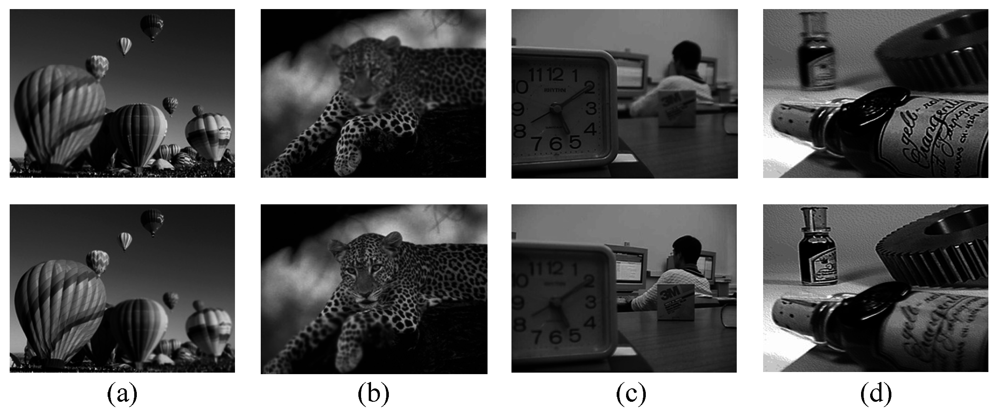
29]. All standard multi-focus images used in this paper are free to use for research purposes. The images from the image fusion library have the size of 256 × 256 pixels or 320 × 240 pixels. The fused images are evaluated by comparing them to the fused images of other existing methods. In this paper, four pairs of images are used as a case study to simulate the proposed multi-focus image fusion method. To simulate a real world environment, four pairs of images have two scenes. One is an outdoor scene, such as a hot-air balloon and leopard shown in Figure 3a,b respectively. The other is an indoor scene, such as a lab and bottle shown in Figure 3c,d respectively. These four pairs of original images are from the same sensor modality. Since each image focuses on a different object, there are two images for each scene. The out-of-focus regions in the original images are blurred.

3.1. Experiment Setup

The quality of the proposed image fusion scheme is evaluated against the other seven popular multi-focus fusion methods. These multi-focus fusion methods consist of popular spatial-based image fusion methods, like Laplacian energy (LE) [8]; four states of art MST methods, including disperse wavelet transform (DWT) [30], dual-tree complex wavelet transform (DT-CWT) [31], curvelet (CVT) [13], non-subsampled contourlet (NSCT) [9]; two sparse representation methods, including sparse representation with a fixed DCT dictionary (SR-DCT) [21] and sparse representation with a trained dictionary by K-SVD (SR-KSVD) [32]. The objective evaluation of fused image includes edge intensity (EI) [33], edge retention Q A B / F [34], mutual information (MI) [35,36], and visual information fidelity (VIF) [
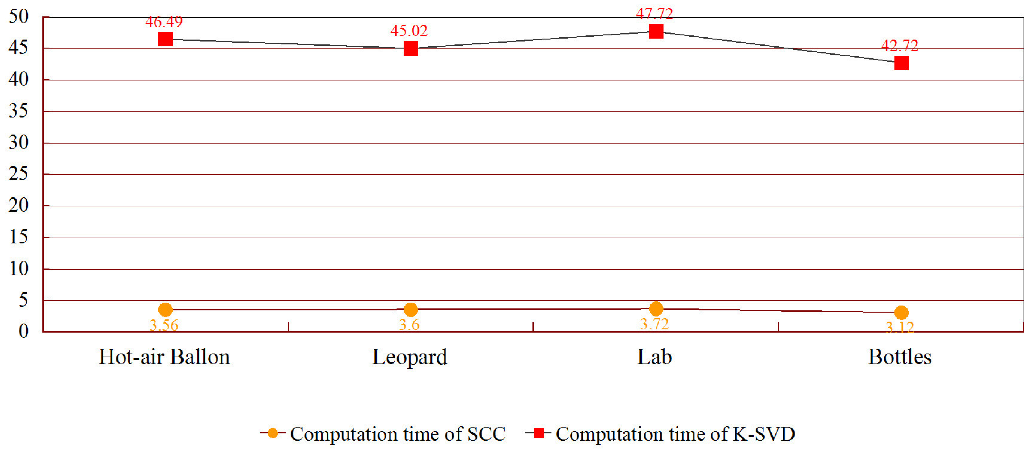
37]. Then it compares the dictionary construction time of the proposed method with K-SVD [32], which is the most popular dictionary construction method. All experiments are implemented using Matlab, version 2014a; MathWorks: Natick, MA, 2014. and Visual Studio, version Community 2013; Microsoft: Redmond, WA, 2013. mixed programming on an Intel(R) Core(TM), version i7-4720HQ; Intel: Santa Clara, CA, 2015. CPU @ 2.60GHz Laptop with 12.00 GB RAM.

3.1.1. Edge Intensity

The quality of the fused image is measured by the local edge intensity L in image I [38]. It folds a Gaussian kernel G with the image I to get a smoothed image. Then it obtains the edge intensity image by subtracting the smoothed image from the original image. The spectrum of the edge intensities depends on the width of the Gaussian kernel G.
L = m a x ( 0 , I G I )
The fused image H is calculated by image L j , j = 1 , , n and the weighted average of local edge intensities.
H ( x , y ) = j = 1 N w j ( x , y ) L j ( x , y ) ,
w j ( x , y ) = L j ( x , y ) k = 1 N L k ( x , y )

3.1.2. Mutual Information

MI for images can be formalized as Equation (14) [35].
M I = i = 1 L j = 1 L h A , F ( i , j ) l o g 2 h A , F ( i , j ) h A ( i ) h F ( j ) ,
where L is the number of gray-level, h R , F ( i , j ) is the gray histogram of image A and F. The h A ( i ) and h F ( j ) are edge histogram of image A and F. For a fused image, the MI of the fused image can be calculated by Equation (15).
M I ( A , B , F ) = M I ( A , F ) + M I ( B , F ) ,
where M I ( A , F ) represents the MI value between input image A and fused image F; M I ( B , F ) represents the MI value of input image B and fused image F.

3.1.3. Q A B / F

The Q A B / F metric is a gradient-based quality index to measure how well the edge information of source images conducted to the fused image [34]. It is calculated by:
Q A B / F = i , j ( Q A F ( i , j ) w A ( i , j ) + Q B F ( i , j ) w B ( i , j ) ) i , j ( w A ( i , j ) + w B ( i , j ) ) ,
where Q A F = Q g A F Q 0 A F , Q g A F and Q 0 A F are the edge strength and orientation preservation values at location (i,j). Q B F can be computed similarly to Q A F . w A ( i , j ) and w B ( i , j ) are the importance weights of Q A F and Q B F respectively.

3.1.4. Visual Information Fidelity

VIF is the novel full reference image quality metric. VIF quantifies the mutual information between the reference and test images based on natural scene statistics (NSS) theory and human visual system (HVS) model. It can be expressed as the ratio between the distorted test image information and the reference image information, the calculation equation of VIF is shown in Equation (17).
V I F = i s u b b a n d s I ( C N , i ; F N , i ) i s u b b a n d s I ( C N , i ; E N , i ) ,
where I ( C N , i ; F N , i ) and I ( C N , i ; E N , i ) represent the mutual information, which are extracted from a particular subband in the reference and the test images respectively. C N denotes N elements from a random field, E N and F N are visual signals at the output of HVS model from the reference and the test images respectively.
An average VIF value of each input image and integrated image is used to evaluate the fused image. The evaluation function of VIF for image fusion is shown in Equation (18) [37].
V I F ( A , B , F ) = V I F ( A , F ) + V I F ( B , F ) 2 ,
where V I F ( A , F ) is the VIF value between input image A and fused image F; V I F ( B , F ) is the VIF value between input image B and fused image F.

3.2. Image Quality Comparison

To show the efficiency of the proposed method, the quality comparison of fused images is demonstrated. Four pairs of multi-focused images of a hot-air balloon, leopard, lab, and bottle are employed for quality comparison. It compares the quality of fused image based on visual effect, the accuracy of focused region detection, and the objective evaluations. The different images are used to show the differences between fused images and corresponding source images. This paper increases the contrast and brightness of difference images for printable purposes. All difference images are adjusted by using the same parameters.
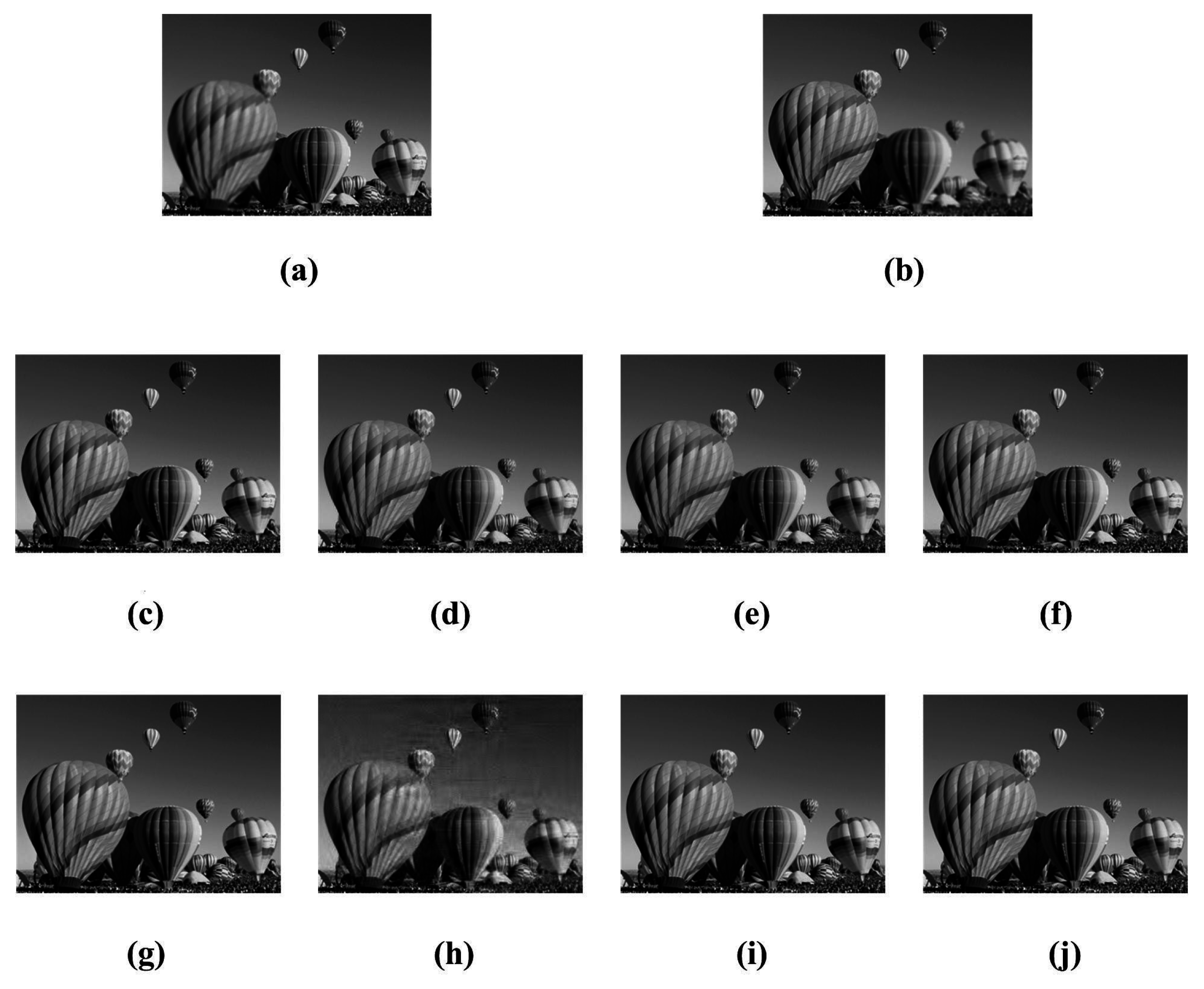
In the first comparison experiment, the "hot-air balloon" images are a pair of multi-focused images. The source multi-focused images are shown in Figure 4a,b. In Figure 4a, the biggest hot-air balloon on the bottom left is out of focus, the rest of the hot-air balloons are in focus. In contrast, in Figure 4b, the biggest hot-air balloon is in focus, but the rest of balloons are out of focus. LE, DWT, DT-CWT, CVT, NSCT, SR-DCT, SR-KSVD and the proposed method are employed to merge two multi-focused images into a clear one, respectively. The corresponding fusion results are shown in Figure 4c–j respectively. The difference images of LE, DWT, DT-CWT, CVT, NSCT, SR-DCT, SR-KSVD and the proposed method do the matrix subtraction with the source images shown in 
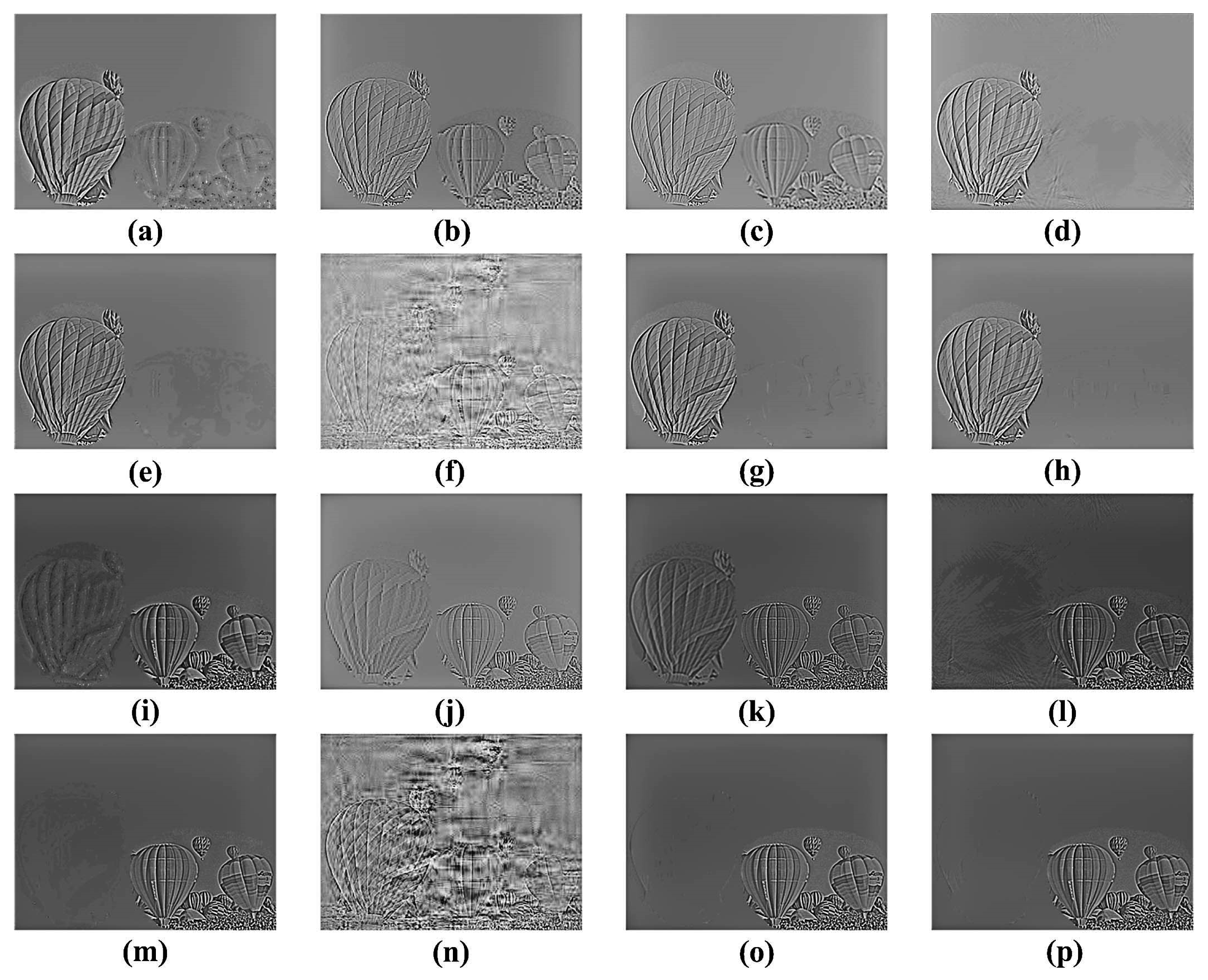
Figure 4a,b. The corresponding subtracted results are shown in Figure 5a–h,i–p respectively.
Figure 5a–h are the difference images between Figure 4a and Figure 4c–j, and Figure 5i–p are the difference images between Figure 4b and Figure 4c–j. The difference images of LE, DWT, DT-CWT, CVT, NSCT, SR-DCT, SR-KSVD and the proposed method are the matrix subtraction results of the corresponding fused images and source images shown in Figure 4a,b.
There are a lot of noises in Figure 4h, which are acquired by SR-DCT. The rest of integrated images in Figure 4 are similar. Difference images, that show hot-air balloons of LE, DWT, and DT-CWT on the left side respectively, do not get all the edge information in Figure 5a–c.
Similarly, Figure 5i–k shows that the biggest hot-air balloons of LE, DWT, and DT-CWT on the bottom left, respectively, are not totally focused. Due to the misjudgement of focused areas, the fused "hot-air balloon" images of LE, DWT, DT-CWT, and SR-DCT have shortcomings. Compared with source images, the rest of the methods do great job in identifying the focused area. To further compare the quality of fused images, objective metrics are used.
Table 1 shows the objective evaluations. Compared with the rest of the image fusion methods, the proposed method SR-SCC gets the largest value in MI and VIF. LE and DT-CWT get the largest value in EI and Q A B / F respectively, but they provide an inaccurate decision in detecting the focused region. The proposed method has the best overall performance of multi-focus image fusion in the "hot-air balloon" scene among all eight methods, according to the quality of fused image, accuracy of locating focused region, and objective evaluations.
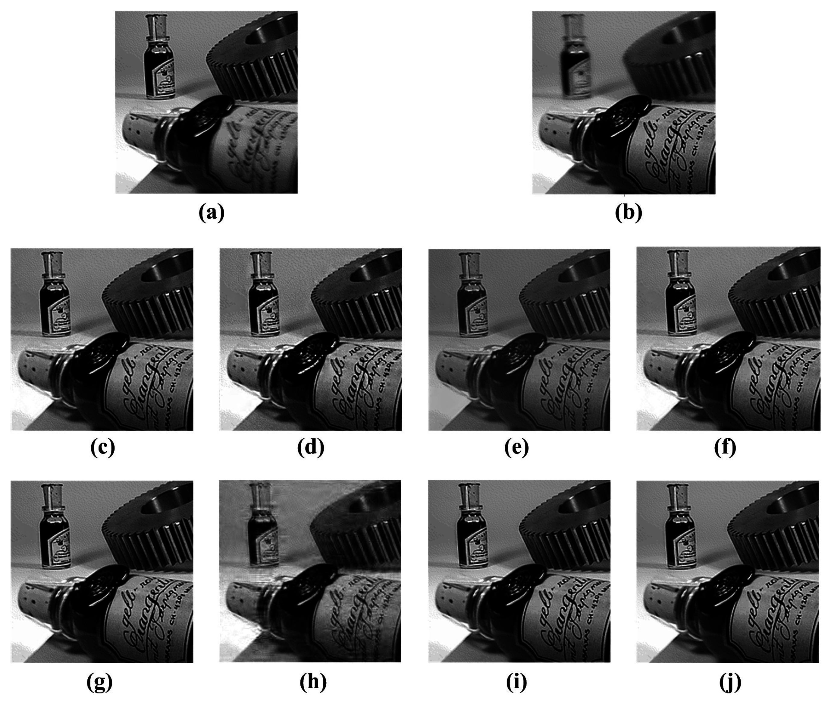
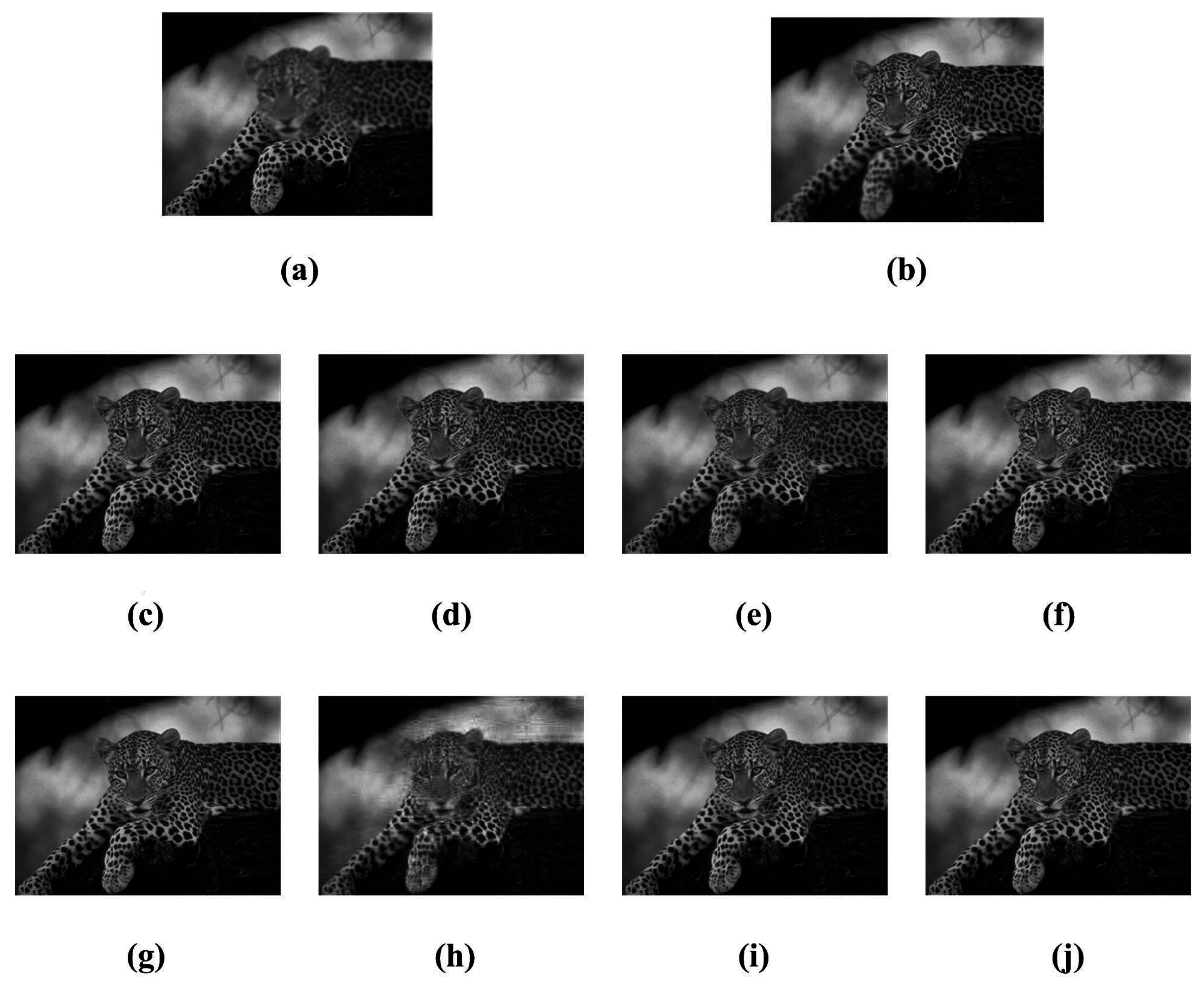
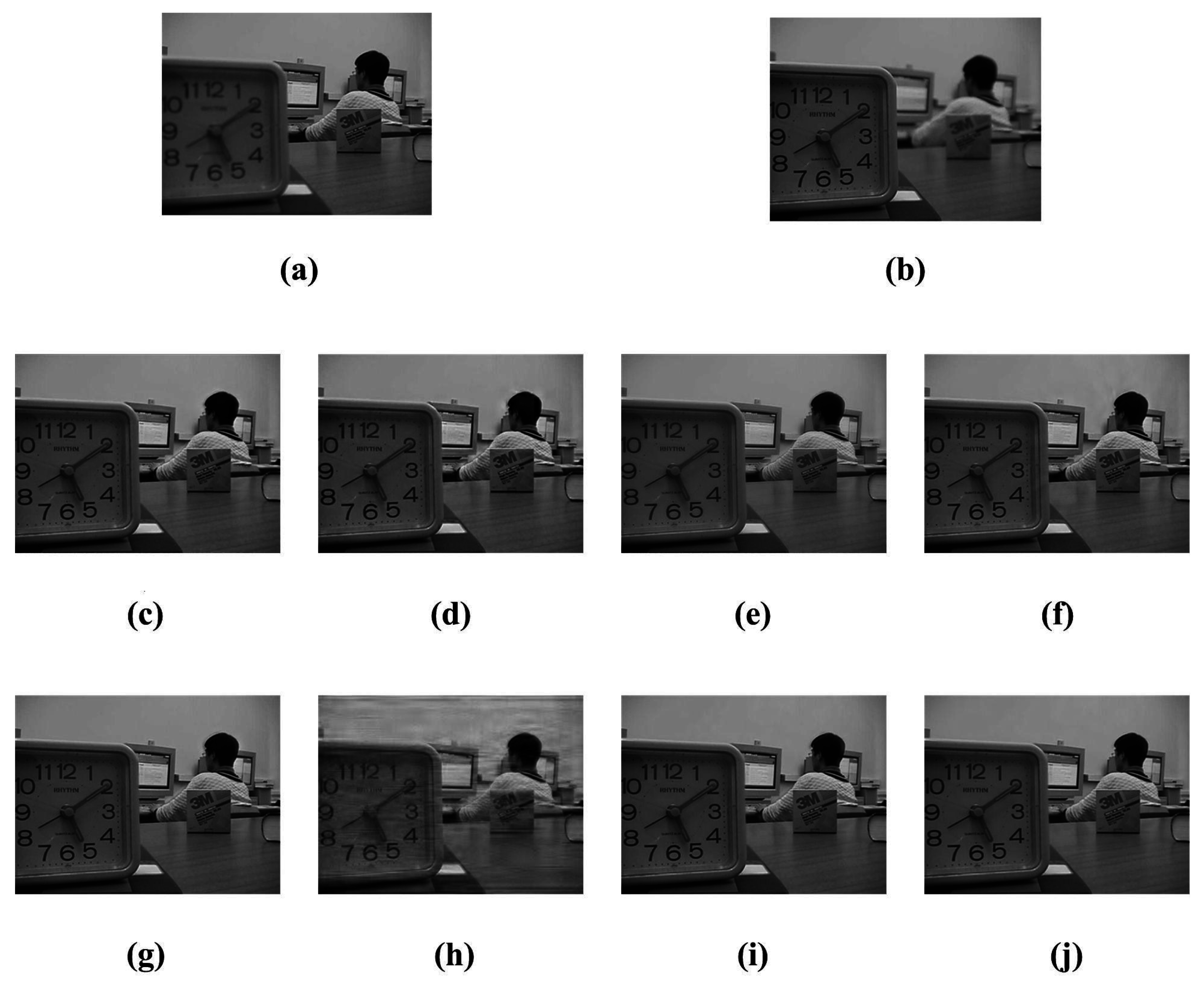
Similarly, the source images of the other three comparison experiments, as "leopard", "lab" and "bottle", are shown in Figure 6, Figure 7 and Figure 8a,b respectively. In a set of source images, two images (a) and (b) focus on different items. The source images are fused by LE, DWT, DT-CWT, CVT, NSCT, SR-DCT, SR-KSVD, and the proposed method to get a totally focused image, and the corresponding fusion results are shown in Figure 6, Figure 7 and 
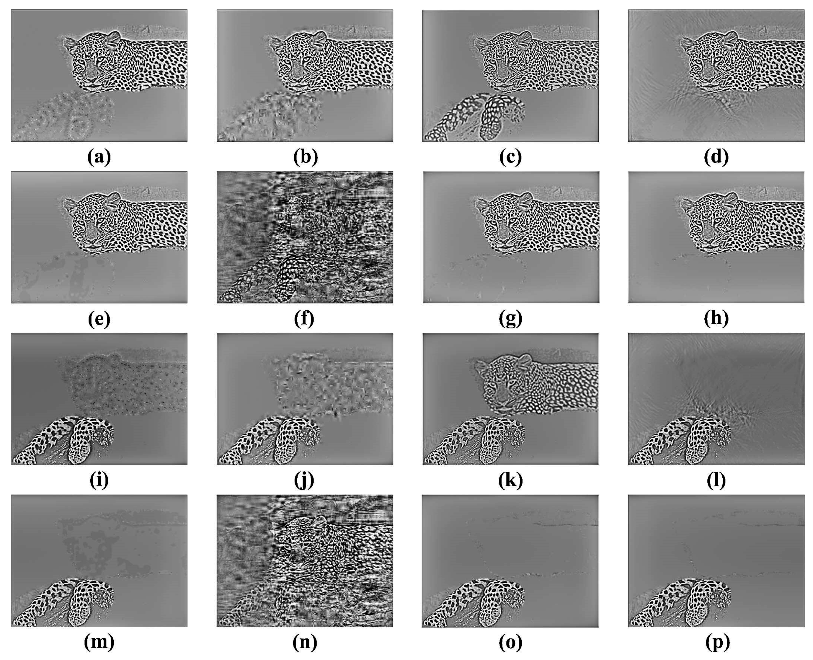
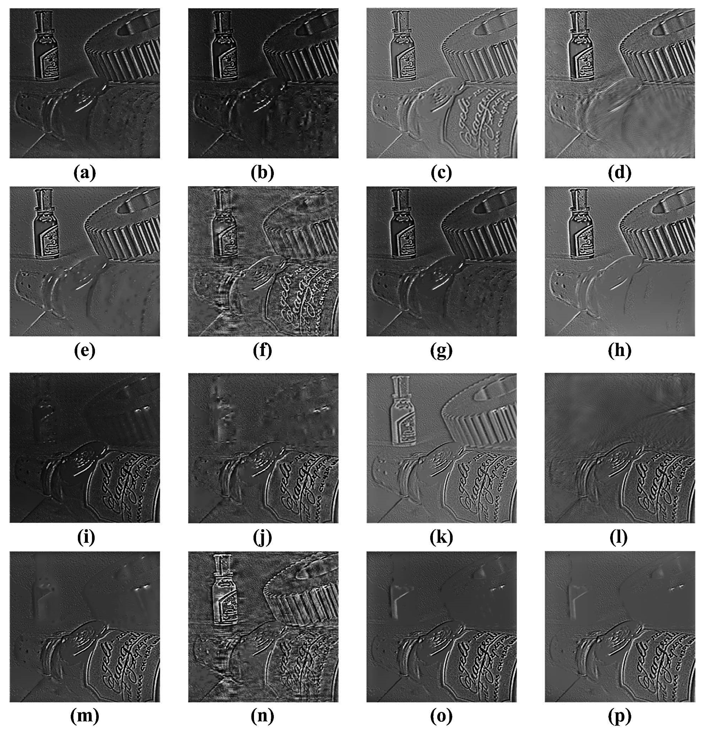
Figure 8c–j respectively. The difference between fused images and their corresponding source images are shown in Figure 9, Figure 10 and Figure 11a–h,i–p respectively.
Objective metrics of multi-focus "leopard", "lab", and "bottle" fusion experiments are shown in Table 2, Table 3 and Table 4 respectively to evaluate the quality of fused images.
  • Multi-focus "leopard" fusion: The proposed method SR-SCC achieves the largest value in MI and VIF. LE obtains the largest value in EI index, but it makes inaccurate decision in detecting the focused region. SR-KSVD shows great performance in Q A B / F , and the result of proposed method is only 0.0002 smaller than SR-KSVD. According to the quality of visual image, the accuracy of focused region, and objective evaluations, the proposed method does a better job than the rest of the methods.
  • Multi-focus "lab" fusion: The proposed method SR-SCC achieves the largest value in Q A B / F and VIF. DWT obtains the largest value of EI index, but it cannot distinguish the correct focused areas. SR-KSVD has the best performance in MI. The proposed method and SR-KSVD show great performance of visual effect in focused area, distinguishing focused area, and objective evaluation. Compared with SR-KSVD, the proposed method dramatically reduces computation costs in dictionary construction. So the proposed method has the best overall performance among all comparison methods.
  • Multi-focus "bottle" fusion: DWT obtains the largest value in EI, but it does not get an accurate focused area. The proposed method achieves SR-SCC with the largest values of the rest of the objective evaluations. So the proposed method has the best overall performance compared with other methods in the "bottle" scene.

3.3. Dictionary Construction Time Comparison

As shown in the previous subsection, the fused images of different multi-focus fusion methods are compared by objective evaluations. Dictionary-learning based image fusion methods, including SR-KSVD and the proposed SCC method, achieve the best performance. However, the dictionary construction process usually takes a very long time. The efficiency of dictionary construction is an important feature of image fusion method. Both K-SVD [39] and the proposed SCC are sparse-representation based dictionary learning methods. So it compares the dictionary construction time of K-SVD and the proposed SCC. K-SVD is one of the most popular dictionary learning methods in recent years. It uses an iterative algorithm to reduce dictionary learning errors and can describe the underlying structure of the image perfectly. To verify the low computation cost of the proposed method, four pairs of images are used for testing computation time. The time consumption of K-SVD and SCC are shown in Figure 12 and Table 5. SCC uses low computation times, that are marked in bold, in four group experiments. The experimental results demonstrate that SCC has a much better performance of computation time than K-SVD.

4. Conclusions

This paper proposed an integrated image fusion framework based on online dictionary learning. Compared with traditional image fusion methods, the integrated framework had two major improvements. First, it introduced a local density-based clustering method in sparse representation, which had high performance in clustering without any apriori knowledge. Second, an online dictionary learning algorithm was used to extract discriminative features that enhanced the efficiency of image fusion. The proposed method was compared with seven existing algorithms LE, DWT, DT-CWT, CVT, NSCT, SR-DCT, SR-KSVD, and SR-SCC using four source image pairs and objective metrics. Experimental results demonstrated that the proposed method was significantly superior to other methods in terms of subjective and objective evaluation. This means that the fused images of the proposed method had better quality than other methods. Compared with other sparse-representation based methods, the proposed method had high efficiency in generating fused images.
Although the proposed solution had a good performance in image fusion, many optimizations are still worth doing in the follow-up research. The parallel processing and the use of multiple graphics processing units (GPUs) will be considered to improve the efficiency of proposed solution. Denoising techniques will also be applied to the proposed solution to enhance the quality of the fused image.

Acknowledgments

We would like to thank the supports by National Natural Science Foundation of China (Nos.61374135, 61203321,61302041), China Central Universities Foundation (106112013CDJZR170005), Chongqing Special Funding in Postdoctoral Scientific Research Project (XM2013007) and Chongqing Funding in Postgraduate Research Innovation Project (CYB14023).

Author Contributions

Zhiqin Zhu and Guanqiu Qi conceived and designed the experiments; Zhiqin Zhu and Guanqiu Qi performed the experiments; Zhiqin Zhu and Guanqiu Qi analyzed the data; Zhiqin Zhu contributed reagents/materials/analysis tools; Zhiqin Zhu and Guanqiu Qi wrote the paper; Yi Chai and Yinong Chen provided technical support and revised the paper.

Conflicts of Interest

The authors declare no conflict of interest.

References

  1. Tsai, W.; Qi, G. DICB: Dynamic Intelligent Customizable Benign Pricing Strategy for Cloud Computing. In Proceedings of the 5th IEEE International Conference on Cloud Computing, Honolulu, HI, USA, 24–29 June 2012; pp. 654–661.
  2. Tsai, W.; Qi, G.; Chen, Y. Choosing cost-effective configuration in cloud storage. In Proceedings of the 11th IEEE International Symposium on Autonomous Decentralized Systems, ISADS 2013, Mexico City, Mexico, 6–8 March 2013; pp. 1–8.
  3. Li, S.; Kang, X.; Hu, J.; Yang, B. Image matting for fusion of multi-focus images in dynamic scenes. Inf. Fusion 2013, 14, 147–162. [Google Scholar] [CrossRef]
  4. Zhu, Z.; Qi, G.; Chai, Y.; Yin, H.; Sun, J. A Novel Visible-infrared Image Fusion Framework for Smart City. Int. J. Simul. Process Model. 2016, in press. [Google Scholar]
  5. Liu, Z.; Chai, Y.; Yin, H.; Zhou, J.; Zhu, Z. A novel multi-focus image fusion approach based on image decomposition. Inf. Fusion 2017, 35, 102–116. [Google Scholar] [CrossRef]
  6. Nejati, M.; Samavi, S.; Shirani, S. Multi-focus image fusion using dictionary-based sparse representation. Inf. Fusion 2015, 25, 72–84. [Google Scholar] [CrossRef]
  7. Kumar, B.K.S. Image fusion based on pixel significance using cross bilateral filter. Signal Image Video Process. 2015, 9, 1193–1204. [Google Scholar] [CrossRef]
  8. Bai, X.; Zhang, Y.; Zhou, F.; Xue, B. Quadtree-based multi-focus image fusion using a weighted focus-measure. Inf. Fusion 2015, 22, 105–118. [Google Scholar] [CrossRef]
  9. Kong, X.L.H.L.Z.Y.Y. Multifocus image fusion scheme based on the multiscale curvature in nonsubsampled contourlet transform domain. Opt. Eng. 2015, 54, 1–15. [Google Scholar]
  10. Lai, Y.; Chen, Y.; Liu, Z.; Yang, Z.; Li, X. On monitoring and predicting mobile network traffic abnormality. Simul. Model. Pract. Theory 2015, 50, 176–188. [Google Scholar] [CrossRef]
  11. Chai, Y.; Li, H.; Li, Z. Multifocus image fusion scheme using focused region detection and multiresolution. Opt. Commun. 2011, 284, 4376–4389. [Google Scholar] [CrossRef]
  12. Tsai, W.T.; Qi, G. Integrated fault detection and test algebra for combinatorial testing in TaaS (Testing-as-a-Service). Simul. Model. Pract. Theory 2016, 68, 108–124. [Google Scholar] [CrossRef]
  13. Bhutada, G.G.; Anand, R.S.; Saxena, S.C. Edge preserved image enhancement using adaptive fusion of images denoised by wavelet and curvelet transform. Dig. Signal Process. 2011, 21, 118–130. [Google Scholar] [CrossRef]
  14. Kim, M.; Han, D.K.; Ko, H. Joint patch clustering-based dictionary learning for multimodal image fusion. Inf. Fusion 2016, 27, 198–214. [Google Scholar] [CrossRef]
  15. Keerqinhu; Qi, G.; Tsai, W.; Hong, Y.; Wang, W.; Hou, G.; Zhu, Z. Fault-Diagnosis for Reciprocating Compressors Using Big Data. In Proceedings of the Second IEEE International Conference on Big Data Computing Service and Applications, BigDataService 2016, Oxford, UK, 29 March–1 April 2016; pp. 72–81.
  16. Dabov, K.; Foi, A.; Katkovnik, V.; Egiazarian, K.O. Image Denoising by Sparse 3-D Transform-Domain Collaborative Filtering. IEEE Trans. Image Process. 2007, 16, 2080–2095. [Google Scholar] [CrossRef] [PubMed]
  17. Dong, W.; Zhang, L.; Shi, G.; Wu, X. Image Deblurring and Super-Resolution by Adaptive Sparse Domain Selection and Adaptive Regularization. IEEE Trans. Image Process. 2011, 20, 1838–1857. [Google Scholar] [CrossRef] [PubMed]
  18. Xu, Z.; Sun, J. Image Inpainting by Patch Propagation Using Patch Sparsity. IEEE Trans. Image Process. 2010, 19, 1153–1165. [Google Scholar] [PubMed]
  19. Yang, J.; Wright, J.; Huang, T.S.; Ma, Y. Image super-resolution as sparse representation of raw image patches. In Proceedings of the 2008 IEEE Computer Society Conference on Computer Vision and Pattern Recognition (CVPR 2008), Anchorage, AK, USA, 24–26 June 2008.
  20. Li, H.; Li, L.; Zhang, J. Multi-focus image fusion based on sparse feature matrix decomposition and morphological filtering. Opt. Commun. 2015, 342, 1–11. [Google Scholar] [CrossRef]
  21. Yang, B.; Li, S. Multifocus Image Fusion and Restoration With Sparse Representation. IEEE Trans. Instrum. Meas. 2010, 59, 884–892. [Google Scholar] [CrossRef]
  22. Wang, J.; Liu, H.; He, N. Exposure fusion based on sparse representation using approximate K-SVD. Neurocomputing 2014, 135, 145–154. [Google Scholar] [CrossRef]
  23. Zhang, A.; Fu, Y.; Li, H.; Zou, J. Dictionary learning method for joint sparse representation-based image fusion. Opt. Eng. 2013, 52, 532–543. [Google Scholar] [CrossRef]
  24. Lin, B.; Li, Q.; Sun, Q.; Lai, M.; Davidson, I.; Fan, W.; Ye, J. Stochastic Coordinate Coding and Its Application for Drosophila Gene Expression Pattern Annotation. arXiv, 2014; arXiv:1407.8147. [Google Scholar]
  25. Rodriguez, A.; Laio, A. Clustering by fast search and find of density peaks. Science 2014, 344, 1492–1496. [Google Scholar] [CrossRef] [PubMed]
  26. Tsai, W.; Colbourn, C.J.; Luo, J.; Qi, G.; Li, Q.; Bai, X. Test algebra for combinatorial testing. In Proceedings of the 8th IEEE International Workshop on Automation of Software Test, AST 2013, San Francisco, CA, USA, 18–19 May 2013; pp. 19–25.
  27. Combettes, P.L.; Wajs, V.R. Signal recovery by proximal forward-backward splitting. Multiscale Model. Simul. 2005, 4, 1168–1200. [Google Scholar] [CrossRef]
  28. Wu, W.; Tsai, W.; Jin, C.; Qi, G.; Luo, J. Test-Algebra Execution in a Cloud Environment. In Proceedings of 8th IEEE International Symposium on Service Oriented System Engineering, SOSE 2014, Oxford, UK, 7–11 April 2014; pp. 59–69.
  29. Image Fusion Examples. Available online: http://www.imagefusion.org (accessed on 27 July 2016).
  30. Zheng, Y.; Essock, E.A.; Hansen, B.C.; Haun, A.M. A new metric based on extended spatial frequency and its application to DWT based fusion algorithms. Inf. Fusion 2007, 8, 177–192. [Google Scholar] [CrossRef]
  31. Anantrasirichai, N.; Achim, A.; Bull, D.; Kingsbury, N. Mitigating the effects of atmospheric distortion using DT-CWT fusion. In Proceedings of the 19th IEEE International Conference on Image Processing (ICIP), Orlando, FL, USA, 30 Sepember–3 October 2012; pp. 3033–3036.
  32. Chen, H.; Huang, Z. Medical Image Feature Extraction and Fusion Algorithm Based on K-SVD. In Proceedings of the 9th IEEE International Conference on P2P, Parallel, Grid, Cloud and Internet Computing (3PGCIC), Guangzhou, China, 8–10 November 2014; pp. 333–337.
  33. Dixon, T.D.; Canga, E.F.; Nikolov, S.G.; Troscianko, T.; Noyes, J.M.; Canagarajah, C.N.; Bull, D.R. Selection of image fusion quality measures: objective, subjective, and metric assessment. J. Opt. Soc. Am. A 2007, 24, B125–B135. [Google Scholar] [CrossRef]
  34. Qu, G.; Zhang, D.; Yan, P. Information measure for performance of image fusion. Electron. Lett. 2002, 38, 313–315. [Google Scholar] [CrossRef]
  35. Xydeas, C.; Petrović, V. Objective image fusion performance measure. Electron. Lett. 2000, 36, 308–309. [Google Scholar] [CrossRef]
  36. Tsai, W.T.; Qi, G.; Zhu, Z. Scalable SaaS Indexing Algorithms with Automated Redundancy and Recovery Management. Int. J. Softw. Inform. 2013, 7, 63–84. [Google Scholar]
  37. Sheikh, H.; Bovik, A. Image information and visual quality. IEEE Trans. Image Process. 2006, 15, 430–444. [Google Scholar] [CrossRef] [PubMed]
  38. Block, M.; Schaubert, M.; Wiesel, F.; Rojas, R. Multi-Exposure Document Fusion Based on Edge-Intensities. In Proceedings of the 2009 10th International Conference on Document Analysis and Recognition, Catalonia, Spain, 26–29 July 2009; pp. 136–140.
  39. Aharon, M.; Elad, M.; Bruckstein, A. SVDD: An Algorithm for Designing Overcomplete Dictionaries for Sparse Representation. Trans. Signal Proc. 2006, 54, 4311–4322. [Google Scholar] [CrossRef]
Figure 1. Proposed Image Fusion Framework.
Futureinternet 08 00053 g001
Figure 2. Local Density and Distance Map of Fusion Images, (a) shows the local density calculation of each image patch; (b) shows the constructed local density map.
Futureinternet 08 00053 g002
Figure 3. Four Source Image Pairs of Different Scenes for Multi-focus Fusion Experiments, (a)–(d) are source image pairs of hot-air balloon, leopard, lab, bottle respectively.
Futureinternet 08 00053 g003
Figure 4. Fused Images of "Hot-air Balloon" by Different Methods, (a,b) are source images, (cj) are fused images of LE, DWT, DT-CWT, CVT, NSCT, SR-DCT, SR-KSVD, and proposed SR-SCC respectively.
Futureinternet 08 00053 g004
Figure 5. Difference Images of "Hot-air Balloon" by Different Methods, (ah) are differences images between source image in Figure 4a and fused images of LE, DWT, DT-CWT, CVT, NSCT, SR-DCT, SR-KSVD, and proposed SR-SCC in Figure 4c–j respectively, (ip) are differences images between source image in Figure 4b and corresponding fused images in Figure 4c–j respectively.
Futureinternet 08 00053 g005
Figure 6. Fused Images of "Leopard" by Different Methods, (a,b) are source images, (cj) are fused images of LE, DWT, DT-CWT, CVT, NSCT, SR-DCT, SR-KSVD, and proposed SR-SCC respectively.
Futureinternet 08 00053 g006
Figure 7. Fused Images of "Lab" by Different Methods, (a,b) are source images; (cj) are fused images of LE, DWT, DT-CWT, CVT, NSCT, SR-DCT, SR-KSVD, and proposed SR-SCC respectively.
Futureinternet 08 00053 g007
Figure 8. Fused Images of "Bottle" by Different Methods, (a,b) are source images; (cj) are fused images of LE, DWT, DT-CWT, CVT, NSCT, SR-DCT, SR-KSVD, and proposed SR-SCC respectively.
Futureinternet 08 00053 g008
Figure 9. Difference Images of "Leopard" by Different Methods, (ah) are differences images between source image in Figure 6a and fused images of LE, DWT, DT-CWT, CVT, NSCT, SR-DCT, SR-KSVD, and proposed SR-SCC in Figure 6c–j respectively, (ip) are differences images between source image in Figure 6b and corresponding fused images in Figure 6c–j respectively.
Futureinternet 08 00053 g009
Figure 10. Difference Images of "Lab" by Different Methods, (ah) are differences images between source image in Figure 7a and fused images of LE, DWT, DT-CWT, CVT, NSCT, SR-DCT, SR-KSVD, and proposed SR-SCC in Figure 7c–j respectively, (ip) are differences images between source image in Figure 7b and corresponding fused images in Figure 7c–j respectively.
Futureinternet 08 00053 g010
Figure 11. Difference Images of "Bottle" by Different Methods, (ah) are differences images between source image in Figure 8a and fused images of LE, DWT, DT-CWT, CVT, NSCT, SR-DCT, SR-KSVD, and proposed SR-SCC in Figure 8c–j respectively, (ip) are differences images between source image in Figure 8b and corresponding fused images in Figure 8c–j respectively.
Futureinternet 08 00053 g011
Figure 12. Computation Time Comparison.
Futureinternet 08 00053 g012
Table 1. Objective Evaluations of Multi-focus "Hot-air Balloon" Fusion Experiments.
MethodEI Q AB / F MIVIF
LE70.50690.98437.13590.7829
DWT64.29230.94656.85320.7463
DT-CWT63.56880.98786.88280.7771
CVT69.62410.98127.15790.8113
NSCT69.49870.98507.60920.8187
SR-DCT65.96020.74883.92200.4695
SR-KSVD69.51900.98547.88240.8234
SR-SCC69.56250.98527.91170.8242
Table 2. Objective Evaluations of Multi-focus "Leopard" Fusion Experiments.
MethodEI Q AB / F MIVIF
LE94.13430.94436.76770.7920
DWT94.80930.94306.17650.7629
DT-CWT80.26430.94706.20830.7636
CVT93.57360.93596.41090.8068
NSCT93.67670.94477.19400.8245
SR-DCT76.99350.73433.30020.7291
SR-KSVD93.52760.94507.46070.8269
SR-SCC93.64480.94487.54200.8283
Table 3. Objective Evaluations of Multi-focus "Lab" Fusion Experiments.
MethodEI Q AB / F MIVIF
LE55.09260.79645.07240.6299
DWT56.72620.87954.66650.5885
DT-CWT44.64700.81965.09990.6025
CVT53.57110.84384.79370.6367
NSCT53.59580.80555.31110.6625
SR-DCT48.87650.63323.11220.3385
SR-KSVD53.04610.87915.73450.6766
SR-SCC53.03040.88265.66560.6893
Table 4. Objective Evaluations of Multi-focus "Bottle" Fusion Experiments.
MethodEI Q AB / F MIVIF
LE128.05120.84784.10590.4113
DWT131.50330.83553.56960.3779
DT-CWT96.31710.85483.80490.4035
CVT122.56160.84483.87990.4678
NSCT69.49870.98507.60920.8187
SR-DCT122.48060.85184.17660.4784
SR-KSVD128.41250.86254.84100.5118
SR-SCC128.51060.86294.89010.5291
Table 5. Time Consumption Comparison.
MethodHot-Air BalloonLeopardLabBottle
K-SVD46.4945.0247.7242.72
SCC3.563.603.723.12

