An Integrated Dictionary-Learning Entropy-Based Medical Image Fusion Framework


1
Collaborative Innovation Center for Industrial Internet of Things, College of Automation, Chongqing University of Posts and Telecommunications, Chongqing 400065, China
2
School of Computing, Informatics, and Decision Systems Engineering, Arizona State University, Tempe, AZ 85287, USA
*
Author to whom correspondence should be addressed.
Future Internet 2017, 9(4), 61; https://doi.org/10.3390/fi9040061
Submission received: 29 August 2017
/
Revised: 20 September 2017
/
Accepted: 29 September 2017
/
Published: 6 October 2017
Abstract
:Image fusion is widely used in different areas and can integrate complementary and relevant information of source images captured by multiple sensors into a unitary synthetic image. Medical image fusion, as an important image fusion application, can extract the details of multiple images from different imaging modalities and combine them into an image that contains complete and non-redundant information for increasing the accuracy of medical diagnosis and assessment. The quality of the fused image directly affects medical diagnosis and assessment. However, existing solutions have some drawbacks in contrast, sharpness, brightness, blur and details. This paper proposes an integrated dictionary-learning and entropy-based medical image-fusion framework that consists of three steps. First, the input image information is decomposed into low-frequency and high-frequency components by using a Gaussian filter. Second, low-frequency components are fused by weighted average algorithm and high-frequency components are fused by the dictionary-learning based algorithm. In the dictionary-learning process of high-frequency components, an entropy-based algorithm is used for informative blocks selection. Third, the fused low-frequency and high-frequency components are combined to obtain the final fusion results. The results and analyses of comparative experiments demonstrate that the proposed medical image fusion framework has better performance than existing solutions.
1. Introduction
High-quality images are often required in application. A high-quality image can help people to increase the accuracy and efficiency of image processing. Image fusion techniques are used to combine multiple images from the same senor modality or different sensor modalities for enhancing visibility. Following the development of cloud computing, cloud environment provides more and more strong computation capacity to process various images [1,2,3].
Imaging technologies are widely used in disease diagnosis, analysis and historical documentation. Image fusion has also aroused research interest in the field of medicine. Medical image fusion is used to fuse multiple images from the same imaging modality or combine information from multiple modalities, such as magnetic resonance image (MRI) [4], computed tomography (CT) [5], positron emission tomography (PET) [6], and single photon emission computed tomography (SPECT) [7].
The fused medical image can reflect medical issues through images of human body, organs and cells. The fused image provides a great diversity of features for medical analysis and diagnosis. Although lots of medical image fusion techniques are available, the quality of fused medical image can still be improved. The unsatisfied fused medical image may affect the interpretation and diagnosis of medical conditions.
A large number of image fusion methods have been proposed for image fusion. Spatial-domain fusion and transform-domain fusion are two typical approaches. Spatial-domain based methods directly choose clear pixels, blocks or regions from source images to compose a fused image without doing any transformation. In general, spatial-domain methods may lead to blurring edges, contrast decrease, and reduction of sharpness [8,9]. Transform-domain based methods decompose source images into coefficients and transform basis first. Then the coefficients are fused by fusion rules. Finally, the fused coefficients and transform basis are inversely transformed to obtain a fused image. It is difficult to select an optimal transform basis without a priori knowledge.
Sparse-representation-based methods are introduced to transform-domain fusion methods to recover a visually appealing reconstruction of the original signal. Sparse-representation based methods can adaptively transform input images without priori knowledge by using trained basis. Based on the adaptively learning feature, images and signals can be described and reconstructed efficiently. Sparse-representation is widely applied to image denoising [10], image deblurring [11], image inpainting [12], super-resolution [13], and image fusion [14,15].
The following three classical sparse-representation based methods improve the learning efficiency of original sparse coding problems. The K-means generalized singular value decomposition (K-SVD) algorithm, as a representative dictionary learning method, focuses on efficiently learning an over-complete dictionary to maximize the image reconstruction power [16,17]. Lee solved the optimization function to speed up the sparse coding algorithm [18]. Based on stochastic approximations, an online dictionary learning method was proposed by Mairal to process the large size dataset efficiently [19,20,21].
Yang and Li [15] first applied the sparse-representation theory to an image fusion field. A joint sparse-representation image fusion method was proposed by Zhang and Fu [22]. Although the image fusion method had lower complexity than K-SVD, it still required a substantial amount of computations. Kim and Han [23] proposed a joint-clustering based dictionary construction method for image fusion that used K-means clustering to group the image patches before dictionary learning. However, it is difficult to get the cluster centers accurately for K-means clustering.
The spatial domain-based methods cannot handle the issues of blurring edges, contrast decrease, and reduction of sharpness well. The transform domain-based methods depend on priori knowledge, but priori knowledge is difficult to obtain. The current solutions more or less have some drawbacks in image fusion, such blur, noise and so on [23,24]. Medical diagnosis has high requirements regarding the quality of the fused image. Even a small flaw may cause serious error in medical diagnosis. So it is important to enhance the quality of fused medical images.
This paper proposes a novel integrated medical image fusion framework. The framework has two parts to do medical image fusion. The source image is discriminated as low-frequency and high-frequency components, and they are fused separately. Two fused images are merged to obtain the final image.
There are many ways to discriminate the source image. Multi-scale transform (MST) is usually used to do the classification. MST can decompose source image, and use the corresponding image fusion algorithm to fuse the decomposed image components. However, the MST computation cost is much higher than other methods. MST takes about 5–10 s to process a 256 × 256 image on a 2.3 GHZ CPU machine. However, Gaussian filter only takes less than one second to process the same size image. Gaussian filter can successfully decompose image components into high-low frequency image components. At the same time, the image noises are classified as high-frequency image components in the decomposition. This can help in the image denosing during the sparse-representation based fusion of high-frequency image components. Comparing with Gaussian filter, MST is not able to process the image denoising. Gaussian filter does image decomposition in spatial-domain. The results of Gaussian filter are low-frequency components that are the non-detailed parts of the image. The high-frequency components, which are the detailed parts of the image, are obtained by deducting the low-frequency components from source image. The weighted average method decreases the contrast and sharpness of image details, and blurs edges, but it processes the non-detailed image information well. Sparse representation has high performance in representing the details of image, so it is used in high-frequency components.
L2-norm can be independently applied over the data mismatch and the regularization terms. It is robust against the noise and outliers and also has good preserving edges (non-smooth optimization). L2-norm can obtain the high precision of image fusion in low-frequency components. So an L2-norm based weighted average method is implemented to low-frequency components fusion. This method calculates the L2-norm of corresponding high frequency components as weight for weighted average components fusion. The fusion performance in non-detailed information, such as blurring edges, contrast and sharpness can be enhanced.
An online dictionary-learning based method is implemented to improve detailed information fusion performance. For ensuring the group sparsity as well as the local structure of atoms in group, the sparse representation method is used to represent the form of clusters and construct a dictionary. According to the current research achievements, dictionary-learning based image fusion approaches with a well-constructed dictionary can have great performance in showing details of source images [24,25,26]. MST-based dictionary-learning method may cause the spatial inconsistency in some smooth area of the fused image by directly using trained dictionary and “Max-L1” fusion scheme [27]. Comparing with other types of images, medical image has its own special features. Usually the margins of medical image are in black and contain limited information. However, those marginal image patches affect the accuracy of dictionary learning. So these image patches are removed and only the remaining informative image patches are used for dictionary learning.
The proposed framework has four steps:
- Step 1 is a denoising process. Each input source image is smoothed by Gaussian filter that is robust to noise. Gaussian filter decomposes detailed information and noises from low-frequency image components. It ensures that high-frequency image components only contain detailed information and noises. It can adjust the sparse coefficients in sparse representation to achieve the image denoising. So sparse-representation based image fusion of high-frequency components can complete image denoising and fusion.
- Step 2 is a decomposition process of low-frequency and high-frequency components. The high-frequency components of each source image can be obtained, by subtracting the low-frequency components of original input source image. The low-frequency components only contain the source image information without details, and the high-frequency components include the detailed information of source image and noises.
- Step 3 is an image fusion process. L2-norm based weighted average method and an online dictionary-learning algorithm are applied to low-frequency and high-frequency components respectively.
- Step 4 is an integration process. The integrated image is obtained by merging the fused images of low-frequency and high-frequency components together.
The contributions of this paper are as follows:
- The low-frequency and high-frequency components of source image are discriminated by Gaussian filter and processed separately.
- An information-entropy based approach is used to select the informative image blocks for dictionary learning. An online dictionary-learning based image fusion algorithm is applied to fuse high frequency components of source image.
- An L2-norm based weighted average method is used to fuse low frequency components of source image.
2. Related Works
2.1. Image Fusion
In many image-processing scenarios, high spatial and high spectral information are required in a single image. Due to observational constraints, current instruments cannot obtain complete information. The image fusion technique is proposed to combine all relevant or complementary information from two or more source images into a single image [27]. The fused image has more information that any of the source images.
Spatial-domain fusion methods directly analyze source images to choose clear pixels, blocks or regions to compose the fused image. Energy of Laplacian and spatial frequency are two typical methods to measure the clarity of pixels or regions. Based on the image clarity measurement, those pixels or regions with higher clarity are selected to construct the fused image. Misalignment and incorrect location of focused objects constrain the performance of spatial-domain fusion methods. For decreasing the constraints, averaging and max pixel schemes perform on a single pixel to generate a fused image. However, the contrast and edge intensity of the fused image may decrease.
Weighted average method, independent component analysis (ICA) [28], principal component analysis (PCA) [29], and brovey transform [30] are typical spatial-domain fusion methods. Spatial-domain fusion methods do spatial distortions by using localized spatial features, such as spatial gradient, spatial frequency and information entropy. However, the spatial features cannot fully reflect the image information, so spatial-domain fusion methods cannot obtain fused images in good quality.
To improve the performance of a fused image, scientists have proposed block-based and region-based algorithms. Tang proposed an image fusion method in discrete cosine transform domain, that divided a source image into 8 by 8 pixel blocks first and then employed a contrast measure to merge the divided blocks [31]. Li proposed a scheme to divide image into blocks and chose the blocks by comparing their spatial frequencies (SF); the fused results are produced by consistency verification [32]. An averaging or max pixel scheme is performed on the single pixel to generate fused image. Although block-based algorithms improve the fusion performance in expressing details of a fused image, the sharpness of the fused image may still be undesirable. Block-based algorithms may cause a block effect, when they are applied to spatial-domain based methods.
Transform-domain fusion methods first transfer source images into frequency domain and then fuse the corresponding coefficients. Many different mathematical transforms are proposed to enhance the performance of the image fusion. Multi-scale transform (MST) algorithms, as a conventional transformation approach, are used to decompose the source images. Wavelet transform basis, shearlet basis, curvelet basis, dual tree complex wavelet transform basis, non-subsampled contourlet transform (NSCT) basis are usually used for MST-based methods. Without a priori knowledge, it is difficult to select an optimal transform basis. Transform-domain based methods cannot give a general solution to fit all source images. The context of source image is closely related to the performance of transform-domain methods. Pyramid and wavelet transforms are used for multi-resolution image fusion [33]. Combination of complex contourlet transform with wavelet can obtain robust image fusion [34]. Transform-based methods can be applied to liver diagnosis [35], prediction of multifactorial diseases [36], parametric classification [36], and multi-modality image fusion [37,38].
2.2. Sparse Representation and Dictionary Learning
In signal processing, sparse representation is an extremely powerful way to acquire, represent and compress high-dimensional signals. According to the sparse representation theory, an image can be sufficiently reconstructed as a linear combination of the fewest possible atoms or transform bases in an over-complete dictionary [23]. The number of atoms in an over-complete dictionary is more than the dimension of signal, and can be used to represent more flexible and meaningful information. For instance, an image can be represented using fixed bases (i.e., Fourier, Wavelet), or concatenations of such bases. Sparse representation provides efficient compression and denoising estimators with simple diagonal operators to address the signal’s natural sparsity [39]. The discrimination power of the discriminative methods with the reconstruction property and the sparsity of the sparse representation is combined [40].
A fixed dictionary can be easily obtained, but it depends on the data type. However, it is difficult to select a good adaptive over-complete dictionary for sparse representation-based image reconstruction and fusion techniques. DCT basis and wavelet basis are often used to form an over-complete dictionary that does not rely on input images.
For dictionary-based image restoration, it is important to build a bridge between sparse representation and dictionary learning. Aharon [16] proposed an adaptive dictionary learning method called K-SVD that is related to the alternate minimization strategy MOD [41]. The dictionary is learned with the extracted patches either from globally or adaptively trained dictionary by applying SVD operations. The non-zero coefficients of the matrix are updated in dictionary update step at the same time. Comparing with the fixed dictionary based methods, K-SVD usually shows a better performance in image reconstruction.
However, it takes high computational costs to do the iterative K-SVD learning processing, especially with the large number of training images. So the dimension of dictionary is constrained. For a certain type of source images, image fusion can also have good performance based on the fixed dictionary. Rubinstein [42] proposed a sparse K-SVD method to learn a sparse dictionary as a type of dictionary between fixed and trained dictionary. Each atom of the leaned sparse dictionary can be represented over a prespecified base dictionary.
Based on the signal sparse representation theory, Yang [43] proposed a novel image fusion scheme that conducted the sparse representation on overlapping patches instead of the whole image by using a small size of dictionary. As the key technique of the proposed solution, the simultaneous orthogonal matching pursuit technique sparsely decomposed different source images into the same subset of dictionary bases. Most of multi-focus image fusion solutions are subject to one or more of image fusion quality degradations, such as blocking artifacts, contrast decrease, sharpness reduction and so on. Nejati [44] utilized a dictionary learned from local patches of source images to do multi-focus image fusion in spatial domain. The corresponding pooled features were extracted by pooling sparse representations of relative sharpness pixels together, according to the learned dictionary. The pooled features are correlated with sparse representations of source images to get the corresponding pixel level score for the decision map of fusion. Markov Random Field (MRF) optimization regularized the decision map.
Clustering of nonlocal patches is introduced to dictionary learning method. A centralized sparse representation (CSR) framework is proposed by Dong that integrates local dictionary learning and nonlocal structure clustering [45]. PCA is used to learn an orthogonal dictionary for each cluster of input patches. All patches are sparsely encoded, and the decomposition coefficients of each cluster are close to a per-cluster mean representation.
Since a small local dictionary as a subset of the global dictionary can be used to describe patch images, Chatterjee [46] proposed a clustering-based denoising method with locally learned dictionaries. A dictionary is iteratively trained by obtaining principal components of each cluster that reflect representative local features of source image.
Mairal [19] proposed an online dictionary learning method based on stochastic approximations to minimize the expectation with respect to the unknown probability distribution of input data. It uses a stochastic version of the majori-zation-minimization principle to do the calculation [47]. A quadratic surrogate of the expected cost is sequentially built and minimized at every iteration.
Stochastic gradient descent algorithm, as an effective way of dictionary learning, was proposed by Olshausen and Field in 1996 [39]. It described gradient steps with a fixed step size computed on mini-batches of the training set and rescaled heuristic gradient to prevent the norm of the columns to grow out of bounds by taking the implicit constraint into account. However, it is actually difficult to choose the suitable step sizes in a data-independent manner.
One classical approach of dictionary learning is the alternate minimization scheme optimizes dictionary learning process [41,48]. It alternates two minimization steps: one with respect to dictionary D with the fixed sparse code A, and one with respect to A with fixed D. Although it is not as fast as a well-tuned stochastic gradient descent algorithm in practice, it is parameter-free.
Learning a compact and representative dictionary is very important for sparse representation. Qiu [49] adopted the rule of maximization of mutual information to learn a compact and discriminative dictionary for action attributes. Siyahjani [50] learned a context aware dictionary to improve the recognition and localization of multiple objects in images. Other methods improve the dictionary performance by separating the particularity and commonality [51] and adding discrimination constraints [52,53]. Most of these methods consider the discrimination between classes, while seldom involving relationships between samples or the local information in the data space.
2.3. Medical Image Fusion
Medical image fusion involves specific imaging modality, clinical problem, doctors and patients. There are three major focused areas of medical image fusion.
2.4. CT and MRI Images Fusion
CT and MRI are important techniques. Due to the differences of the imaging principle, they generally contain complementary and occasionally inconsistent information. Although CT image affords dense structures like bones and implants without introduction of distortion or loss of information, it cannot detect physiological changes. In contrast, an MRI image can support normal and pathological soft tissues information, but it cannot sustain bones information. As supplementary effects of CT and MRI, multi-modality medical image fusion based on compressive sensing can be competent to support accurate clinical requirements that are not apparent in separate source images.
2.5. MRI and PET Image Fusion
MRI-PET (Positron Emission Computed Tomography) is a novel imaging modality that combines anatomic and metabolic data acquisition. MRI image can give the clear soft-tissue image and PET image can construct a three-dimensional image of tracer concentration within the body. The advantage of MRI-PET fusion is registration of the two modalities. It can not only largely replace PET-only scanners in clinical routine, but also expand considerably the clinical and research roles.
2.6. MRI and SPECT Image Fusion
MRI-SPECT (Single-Photon Emission Computed Tomography) is a multi-modalities medical image fusion method that combines structural and functional information from source images. MR as a structural imaging method is used in neuro-image diagnosis. As morphologic changes are used to interpret MR images, MR images usually have low accuracy and poor discrimination in showing diseases. As a functional imaging method, SPECT can reflect metabolic changes. However, without structural information, it is difficult to understand metabolic changes. For improving the utilization of SPECT images in medical diagnosis, structural information needs to link to corresponding metabolic changes.
3. Proposed Framework
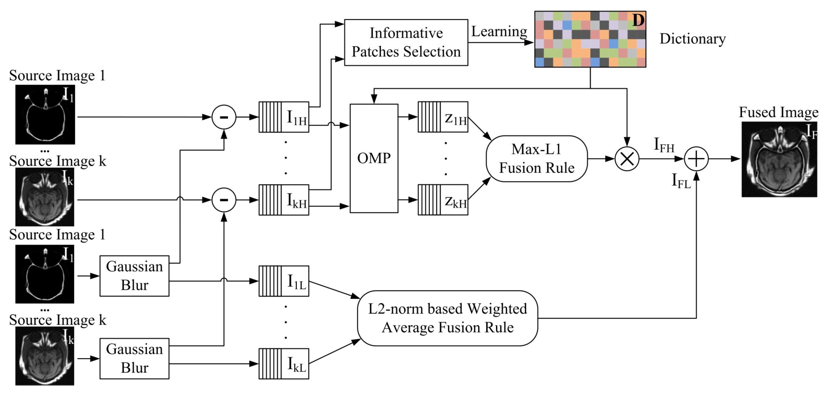
The framework is shown in Figure 1, where to represent the input source image 1 to k.
to and to are high-frequency and low-frequency components of image 1 to k, respectively. to are the sparse coefficients of to . The sparse coefficients to are from to by sparse coding with a constructed dictionary . and are the fused high-frequency and low-frequency components respectively. As shown in Figure 1, the framework consists of three steps. In the first step, input source images are smoothed by the Gaussian filter. These Gaussian smoothed source images are recognized as low-frequency components of input source images. Then the high-frequency components , can be got by subtracting the low-frequency components of original input source image . In the second step, the low-frequency components are fused by an L2-norm based weighted average method. For the high-frequency components, it uses a K-SVD algorithm to build the dictionary. Before the dictionary learning process, an information-entropy based approach is conducted for selecting the informative image blocks. These informative image blocks are used for dictionary learning, that can make the trained dictionary more informative. With the constructed dictionary, high-frequency components are sparse coded to a few sparse coefficients by orthogonal matching pursuit (OMP) algorithm. The sparse coefficients fused by “Max-L1” coefficient fusion rule. In the last step, the fused low-frequency and high-frequency components merged to the fused image .
If the high-low image components are not decomposed, “Max-L1” used for fusing sparse coefficients may select the wrong coefficients and cause an error in the fused image [24]. The decomposition of high-low image components was used by Liu in image fusion. Source images were decomposed into high-low frequency image components, when he did sparse-representation based image fusion [27].
3.1. Gaussian-Filter Based Decomposition
Gaussian filter (also known as Gaussian smoothing) is an effective method that is widely used in image processing to reduce image noise and reduce detail. Gaussian smoothing is often used as a pre-processing stage in computer vision algorithms in order to enhance image structures in different scale-space representation [57,58,59]. Gaussian filter is a low pass filter that has good effect of reducing the image’s high-frequency components. So Gaussian filter is widely used in image fusion for decomposing source images into low-frequency and high-frequency components.
The proposed fusion method processes high-frequency and low-frequency components of source images separately. Then the fused results of high-frequency and low-frequency components are merged. The low-frequency components contain structural information, and contour information to constitute the base of an image. The high-frequency components give the details of an image. The high-frequency components are added upon the low-frequency components to refine the image. It is important to decompose high-frequency and low-frequency components of source images accurately and completely. The accuracy and completeness of decomposition directly affects the fusion result. Only accurate and complete image decomposition can ensure the fused image contains more detailed information. Gaussian filter can decompose the detailed information and noises of source image into high-frequency components [60]. The sparse-representation based solution not only denoises, but also enhances the detailed information of fused image.
In this paper, a two-dimension Gaussian function is used for smooth. The Gaussian function is shown in Equation (1).
where x is the distance from the origin in the horizontal axis, y is the distance from the origin in the vertical axis, and is the standard deviation of the Gaussian distribution. is variable, that can effect how much does it smooth the picture. The standard deviation of Gaussian filter ranges from 2 to 4 depending on the size and type of source images (e.g., = 3 is usually for over 256 ×256 size image). When applied in a smooth image, it produces a surface whose contours are concentric circles with a Gaussian distribution from the center point. Values from this distribution are used to build a convolution matrix which is applied to the original image. Each pixel’s new value is set to a weighted average of that pixel’s neighborhood [61]. When the Gaussian filter algorithm is implemented as a low-pass filter to smooth the input source image, low-frequency component of the input source image can be got. Then high-frequency component can be got by Equation (2).
where is the input source image and is the high-frequency component. After high-frequency and low-frequency components of the source image are received, different fusion scheme is implemented to them, respectively.
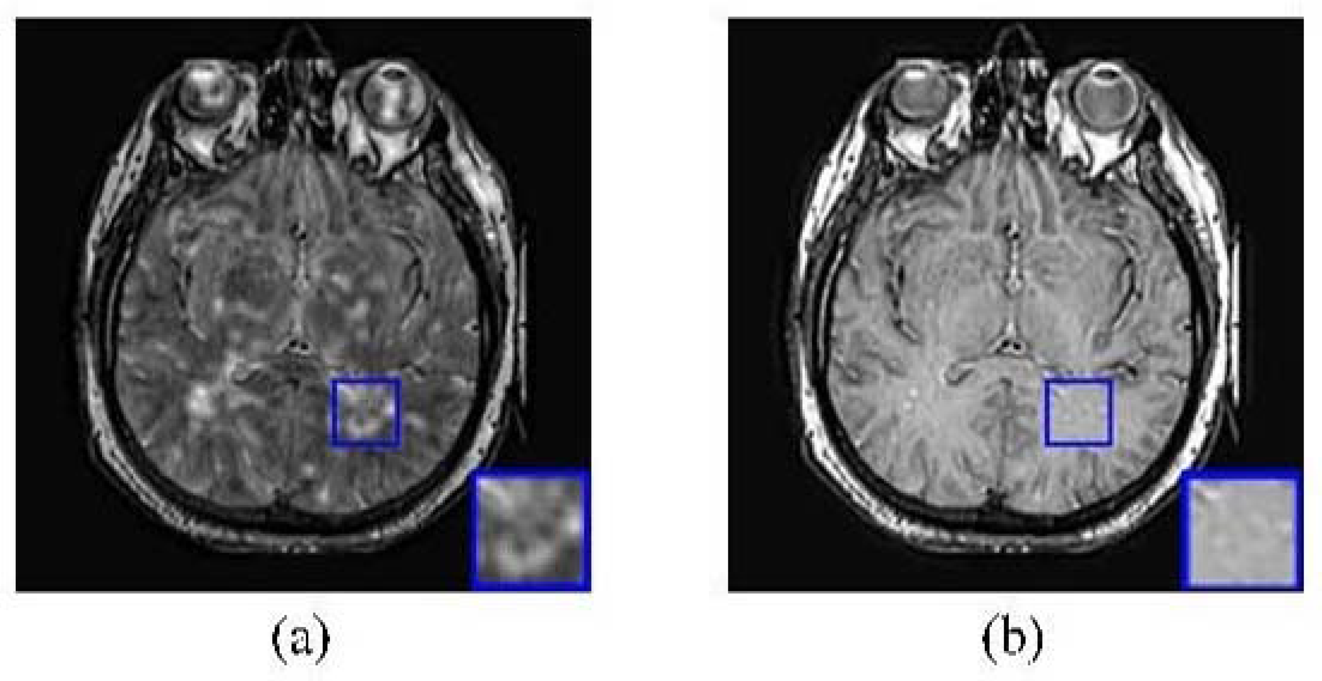
If it does not do the decomposition first, it may misselect the sparse coefficient, and even cause the accuracy of fused result [27]. Source images shown in Figure 2 are used in the comparison of non-decomposition and decomposition. Figure 3a,b show the results of non-decomposition and decomposition respectively. The same pixels marked in blue frame are selected from each result to do the detailed comparison. The result of non-decomposition is blur, but decomposition obtains the clear result.
3.2. High-Frequency Components Fusion
3.2.1. Solution Discussion
The traditional dictionary learning methods use the pixel value to select informative image block. According to the common pixel format, the pixel as the byte image is stored as an 8-bit integer giving a range of possible values from 0 to 255. Zero and 255 are taken to be black and white respectively. Values in between 0 and 255 make up the different shades of gray. Two hundred and fifty five is usually used as a basis to evaluate the pixel value. So the pixel selection may not be accurate. For instance, one pixel and its neighboring pixels may have significant differences. One pixel is bright, but its neighbors are dark. No matter whether a bright or dark pixel is selected, both informative image block selection and the accuracy of learned dictionary are affected.
The gradient-based patch selection approach uses the eigenvalue of edge information to represent source images. Gradient ridges describe positions and shapes of singular structures. Since the local image structure is far more complicated than the parametric representation, it is difficult to model the gradient distribution with a few parameters. Due to the incorrect gradient estimation and no gradient constraint, the reconstructed images are usually over-sharped, suffer from false artifacts, or have a blurring effect.
There is a large set of source image blocks. For dictionary learning, it is difficult to select distinctive image blocks for dictionary construction. The entropy-based patch selection approach evaluates the gray-level probability of each image block, and identifies and selects the most informative image blocks based on the entropy rank (or threshold). Each image block is regarded as relative image information. The entropy calculation process does not depend on a single basis. The pixel numbers of each gray-level image block decide the entropy of each image block. Based on the criterion, the informative image blocks, as a small proportion of source image blocks, are selected.
3.2.2. Dictionary Construction
Dictionary is an important factor in sparse representation. Training a redundant dictionary with small failure rate is a common solution for sparse representation [62,63,64]. However, redundant components of a trained dictionary can cause adverse effects in the accuracy of sparse coding. A certain proportion of redundant elements in the trained dictionary is got from the non-informative blocks in the learning process. As the number of non-informative blocks in medical images is large, using only the informative blocks for learning process can make the trained dictionary productive. To retain the informative blocks and reduce the blocks with limited information, a novel entropy-based informative dictionary construction approach is proposed. The proposed dictionary construction consists of two parts, (1) the informative blocks selection and (2) dictionary learning.
The block-selection approach is based on information entropy, and can be implemented for both gray-level images and color images. Color images are converted to gray-level images for entropy calculation. Supposing input images have w gray-levels, and they are split to n image blocks with pixels, the steps of the selection approach can be demonstrated as follows.
Step 1. Acquiring histogram counts vector of each image blocks by count the pixel numbers of each gray-level. Using and the image blocks size , the gray-levels probability of image block k can be calculated by Equation (3).
Step 2. Calculating the entropy of each image block use gray-levels probability of each image block k. The entropy calculating process is shown in Algorithm 1.
| Algorithm 1 Image Block Entropy Calculation. |
| Input: |
| Gray-levels probability , |
| Output: |
| Entropy of image block, where |
| 1: |
| 2: for i = 1 to S do do |
| 3: Compute the entropy of number ith pixel in image block |
| 4: |
| 5: end for |
Step 3. Reducing the image blocks with low information entropy. In this step, a threshold is set for the informative image blocks selection. For a image block, if , this image block is remained for dictionary learning. On the contrary, if this image block is reduced.
When the informative image blocks are selected, the K-SVD algorithm can be implemented for dictionary learning. The dictionary learning results with all image blocks and only the informative image blocks are shown in Figure 1.
3.2.3. Sparse Coding and Coefficients Fusion
When the dictionary is trained, OMP algorithm is implemented for sparse coding. Supposing input images are split to k image blocks, each image block is coded by OMP algorithm with the input dictionary . Each image block is coded to sparse coefficients . Then the coefficients is fused by “Max-L1” fusion rule. The fusion rule is demonstrated in Equation (4).
where the is the sparse coefficients corresponding to each image patches. is the fused vector, is the norm. “Max-L1” is a fusion algorithm of sparse coefficient that has been widely used in many references [43,65]. This algorithm does the sparse representation of the source image first, then picks the sparse coefficients with large L1 norm as the transformation coefficients, and finally inverts the transformation coefficients to obtain the fused image.
The fused coefficient vectors are restored back to image by Equation (5).
where the , are fused vectors corresponding to the source image patches and is the dictionary trained by the proposed method.
3.3. Low-Frequency Components Fusion
3.3.1. L2-Norm Based Fusion
The weighted average is used to fuse low-frequency components. It assumes that k input images can be split to k low-frequency components and k high-frequency components . It calculates the “L2-norm” of high-frequency components to estimate the percentage of corresponding low-frequency components.
L2-norm as a Euclidean norm is used to measure a vector difference as a standard quantity.
It tries to fine the sparsest solution of the underdetermined linear system that has fewest non-zero entries. The minimization of L2-norm was used to calculate the weights of high-frequency components for the fusion of low-frequency components by Kim [23] and Liu [66]. The L2-norm minimization is formulated by
It assumes the constraint matrix A has full rank. So this underdertermined system has infinite solutions. The lowest L2-norm is one of the best solutions from infinite solutions. For reducing computation costs, Lagrange multipliers are introduced to L2-norm.
where is the introduced Lagrange multipliers. It takes derivative of this equation equal to zero to find a optimal solution and get
Then it substitutes this solution into the constraint to get
Finally, it gets
So it can instantly calculate an optimal solution of L2-norm problem by using the above Equations (7)–(12). Equation (7) is the basic optimization of L2-norm. According to Equation (7), the calculation processes of weighted average of high-frequency components are deduced as Equation (8)–(12).
The calculated corresponding weighted average of each high frequency component is used to fuse low frequency components of source images. The fused low-frequency components can be obtained by
3.3.2. Solution Discussion
High-frequency components correspond to edges in an image. High-frequency components change rapidly, so that an edge is characterized by a sharp change in intensity values. Low-frequency components in an image correspond to smooth regions that represent global information about the shape, such as general orientation and proportions. Low-frequency components change gradually and slowly. The slow change feature would be reflected in the presence of large number of smooth regions. Sharp images have a great proportion of high-frequency components. Oppositely, blurry images have a low proportion of high-frequency components. High-frequency components have been strongly affected, but low-frequency components are unaffected by the blur. According to source images, most of image information is sharp and only a small portion is blurred. The low-frequency components in the small portion, as non-sparse information, are important for image fusion. The appropriate smoothing operation can reduce shape details to delineate the object accurately. It is important to set the threshold for the smoothing operation. The low threshold causes low contrast edges. A variety of new edge points of dubious significance are introduced. The high threshold looses low contrast edges as broken edges.
L1-norm and L2-norm are usually used to transform image signals. L2-norm is more stable than L1-norm. A small perturbation of data points can change the regression line of L1-norm a lot, even its direction. However, L2-norm still maintains the shape of original regression line and only makes a small change in parabolic curve. This means that all future predictions of L1-norm are affected much more seriously than L2-norm predictions.
L1-norm has the built-in feature selection property and tends to produces sparse coefficients. L2-norm does not have this property. For L2-norm, it does not matter whether the source image information can be represented in sparse coefficients.
L2-norm based regularizer produces non-sparse coefficients. The quality of features is one of the most important properties that directly influences the performance of classification. Good-quality features generally enable samples in the same class to stay relatively closer to each other and thus make it easier to generate a discriminative collaborative representation with non-sparse coefficients [67]. Generally speaking, non-sparse representation is more promising than sparse representation in classification. It is robust against noisy and redundant feature sets [67].
Furthermore, L2-norm has analytical solutions, and there is always one solution for the certain data set. L2-norm solutions can be obtained by efficient calculation. Due to the sparsity properties, the L1-norm can use sparse algorithms to obtain the solutions. L1-norm is not efficient to solve non-sparse cases. L1-norm may have multiple solutions. So L1-norm is not efficient to obtain solutions as L2-norm.
3.4. Fused Components Merging
According to fusion rules, the fused high-frequency and low-frequency components are combined to form the final fused image.
3.5. Comparison of Learned Dictionary
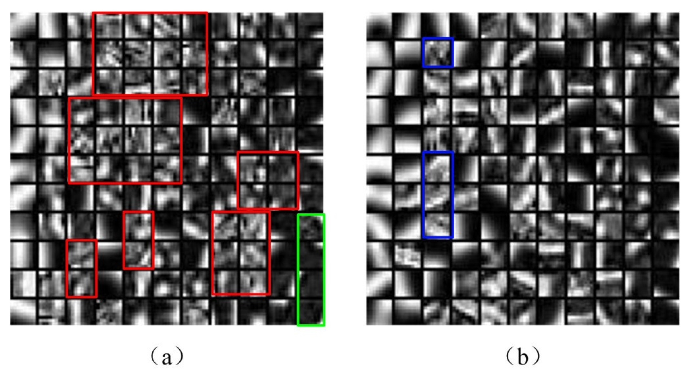
Figure 4a,b show the details of a learned dictionary using traditional and proposed method respectively. The traditional method does not eliminate the non-useful information from source image before doing the dictionary-learning process. In image fusion, the size of the learned dictionary is usually set to 256 or 512. So the learned dictionary by traditional method shown in Figure 4a has too many stochastic blocks marked in red frame. Parts of stochastic blocks marked in the green frame are too dark.
Compared with the traditional method, the proposed solution obtains a better learned dictionary shown in Figure 4b. The proposed solution classifies the source image information into low-frequency and high-frequency components. The image information that contains low-entropy information is eliminated from the dictionary-learning process. In the learned dictionary, the number of stochastic blocks decreases. The majority of the learned dictionary consisted of dominant orientation blocks. Those dominant orientation blocks contain more detailed information of the medical image, such as edge details, edge direction and so on, that can increase the accuracy of medical image fusion.
4. Experiments and Analysis
4.1. Experimental Setup
To further test the efficiency of the proposed framework, nine groups of multi-modality images are conducted for testing. These multi-modality image groups include CT-MRI, MRI-PET, and MRI-SPECT image fusion. All the source images have the size of 256 × 256 pixels and can be obtained at two public websites [68,69]. Figure 5a–i are the source image pairs for CT-MRI, MRI-PET, and MRI-SPECT image fusion experiments, respectively. Only one comparative experiment of each image fusion type is chosen to present in detail, including fused images and objective evaluations. For other comparative experiments, it only shows the average objective evaluations of CT-MRI, MRI-PET, and MRI-SPECT image fusion, respectively. In this paper, the quality of the proposed framework is compared with other existing methods, including BSD (Block-based Spatial Domain) [70], DWT [71], DT-CWT [72], CS-DCT [73], KSVD-OMP [74], Yang’s multi-focus image fusion and restoration solution (MFR) [15], Zhang’s sparse representation-based image fusion solution with dictionary learning (SRDL) [22], Kim’s joint patch clustering-based image fusion solution (JPC) [23] and Liu’s multi-scale transform and sparse representation-based image fusion solution (MST-SR) [27]. SRDL, JPC, and MST-SR used the similar frameworks as our proposed solution respectively to obtain good fusion performance. Based on their solutions, our proposed solution improves in the representation of detailed information, and furtherly enhances the performance of the fused image. The objective evaluation of the fused image includes the AG (Average Gradient) [75], Edge-Intensity (EI) [76], Edge Retention [77], Mutual Information (MI) [78], and Visual Information Fidelity (VIF) [79]. In this paper, the size of the learned dictionary is set to 128, and the size of the image patch is set to 8 × 8. It adjusts the step size of sliding window by allowing at least 75% of the 8 × 8 size patch image as overlapped region in all comparative experiments (i.e., 2-pixel in each vertical and horizontal direction). The error tolerance for all sparse representation-based methods is set to = 0.15. All the experiments are implemented using Matlab 2014a and Visual studio 2013 community on an Intel(R) Core(TM) i7-4720HQ CPU @ 2.60 GHz Laptop with 12.00 GB RAM.
4.2. Image Quality Comparison
To show the efficiency of proposed method, the quality comparison of fused medical images is demonstrated. The proposed method and other five existing methods are implemented in CT-MRI, MRI-PET, and MRI-SPECT medical image fusion. The qualities of fused images are compared based on visual effect and following five objective evaluations.
- AG computes the average gradients of each pixel in fused image, that shows the obvious degree of objects in the image. When AG gets larger, the difference between object and background increases [75].
- EI measures the strength of image local changes [76]. A higher EI value implies the fused image contains more intensive edges.
- edge strength represents the edge information associated with the fused image and visually supported by human visual system [77]. A higher value of value implies fused image contains better edge information.
- MI computes the information transformed from source images to fused images. When MI gets larger, the fused image gets more information from source images [78].
- VIF is a novel full-reference image quality metric [79]. VIF quantifies the information shared between the test and reference images based on the Natural Scene Statistics (NSS) theory and Human Visual System (HVS) model.
According to existing papers, objective evaluation metrics are always used to evaluate the performance of the fused image objectively [15,22,23]. Doctors actually use image information to diagnose the disease. The high-quality fused images are helpful for doctors to make the accurate diagnosis. The above five objective evaluation metrics (AG, EI, , MI, VIF) used in this paper are the internationally common methods to evaluate the performance of medical image fusion [80,81,82].
4.2.1. CT-MRI Image Fusion Comparative Experiments
The ‘brain’ images are a pair of CT and MRI images shown in Figure 6a,b respectively. CT image shows the bone information and MRI image shows soft issues. BSD (Block-based Spatial Domain), DWT, DT-CWT, CS-DCT, KSVD-OMP, MFR, SRDL, JPC, MST-SR, and the proposed method (IDLE) are employed to merge CT and MRI images into a clear one with bone and soft issues information respectively. The corresponding fusion results are shown in Figure 6c–l) respectively.
As BSD is a spatial-domain method, it is easy to figure out block effects in fused image (c). Fused image (d) has good performance in details of high-frequency components, but details of low-frequency components are darker than source images. The contrast and sharpness of the fused image (d) are good. Image (e) fused by DT-CWT has low contrast and sharpness. CS-DCT keeps details of CT and MRI images in the fused image (f), but the contrast and sharpness are low. The fused image (g) of KSVD has good overall performance, but the sharpness of details is not sufficient. MFR keeps the details of source images in the fused image (h). The details in the Fused image (i) of SRDL have low contrast and sharpness. The fused image (j) of JPC shows good detailed information. MST-SR causes the details of low-frequency components to be darker than the source images in the fused image (k). The fused image (l) of proposed IDLE not only contains complete details, but also has good contrast and sharpness.
Then it compares the details of each fused image. Red and blue frame in image (a) and (b) show the important details of bone and soft issues. Block effect affects the corresponding details in fused image (c). In fused image (d), the bone part is too bright and the soft issue part is too dark. The corresponding details of fused image (e) are blurred. This is not good for medical diagnosis (e). The contrast and sharpness of fused image (f) are low. The fused image (f) also has some blurs. The fused image (g) has good brightness, but the contrast is low. Details of source images are shown in the fused image (h) clearly. In the fused image (i), the details of bone part are blurred. The fused image (j) shows clear and complete detailed information. The soft issue part is too dark in the fused image (k). The proposed IDLE generates a fused image (l) that contains complete and clear details and also has good contrast and sharpness.
Table 1 shows the objective evaluations. Compared with the rest of image fusion methods, the proposed IDLE gets the largest value in , MI, and VIF. BSD gets the largest value in AG and EI, but it has block effects in the fused image. So the proposed IDLE has the best overall performance in CT and MRI ‘brain’ image fusion among all 10 methods, according to the quality of fused image, contrast, sharpness and objective evaluations.
4.2.2. MRI-PET Image Fusion Comparative Experiments
The ‘brain’ images are a pair of MRI and PET images shown in Figure 7a,b respectively. The MRI image shows the image of brain slices that contain clear information of soft tissues. The PET image also shows the image of brain slices that produces a 3D image of functional processes in human body. BSD, DWT, DT-CWT, CS, KSVD-OMP, MFR, SRDL, JPC, MST-SR, and the proposed IDLE are employed to merge MRI and PET images into a clear image with soft tissues and functional processes information. The corresponding fusion results are shown in Figure 7c–l respectively.
Similar to SPECT, the results of BSD and DWT have the issue of chromatic dispersion, and this may cause misdiagnosis. So BSD and DWT are not recommended to fuse MRI and PET images. The fused images of DT-CWT and KSVD-OMP have high quality, and both contrast and sharpness are also good. However, the detailed parts of these fused images have low brightness, compared with the proposed IDLE. MFR, SRDL, and JPC show a good performance in fusing source images. The fused image (k) of MST-SR is brighter than the source image. The fused image (l) of proposed IDLE has high quality in details, contrast, sharpness, and brightness.
Table 2 shows the objective evaluations. Compared with the rest of the image fusion methods, the proposed IDLE gets the largest value in , MI, and VIF. DWT gets the largest value in AG and EI, but it has chromatic dispersion issues in fused images. So the proposed IDLE has the best overall performance in PET and MRI image fusion among all 10 methods, according to the quality of fused image, contrast, sharpness, brightness, and objective evaluations.
4.2.3. MRI-SPECT Image Fusion Comparative Experiments
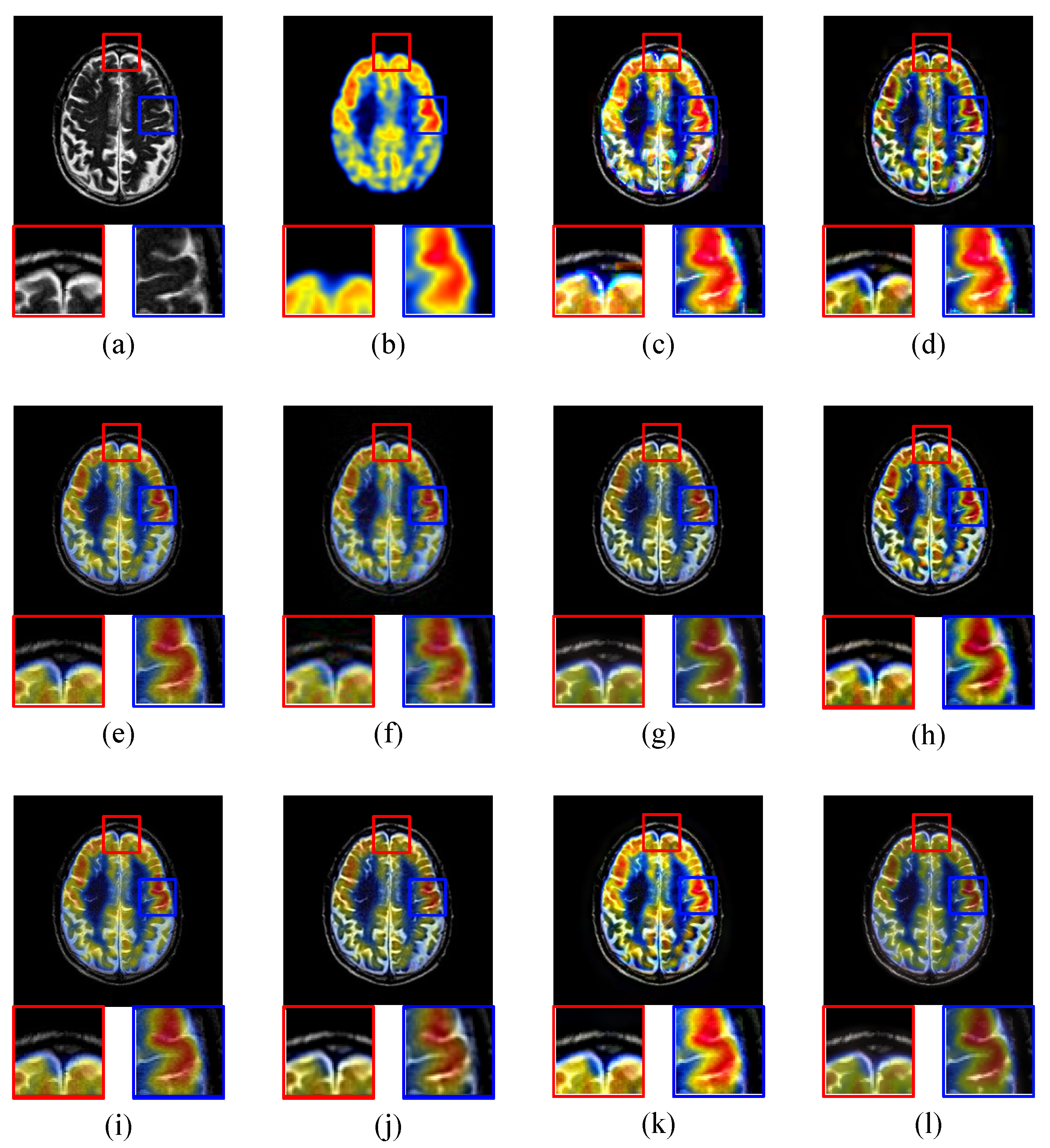
The ‘brain’ images are a pair of MRI and SPECT images shown in Figure 8a,b respectively. Similarly, the MRI image also shows the image of brain slices with soft-tissue information in this experiment. The SPECT image provides the true 3D information of brain slices that is typically presented as cross-sectional slices through the patient, and can be freely reformatted or manipulated as required. BSD, DWT, DT-CWT, CS-DCT, KSVD-OMP, MFR, SRDL, JPC, MST-SR, and the proposed IDLE are employed to merge MR and SPECT images into 3D image with soft-tissue information. The corresponding fusion results are shown in Figure 8c–l respectively.
The fused image (c) obtained by BSD has serious block effects that make the details unclear. The DWT result has a chromatic dispersion that may cause medical misdiagnosis. The fused image of DT-CWT has good performance in contrast, sharpness and details. CS-DCT does not generate the high-quality fused image. The details of the fused image are blurred and contain lots of noises. Although the overall contrast of KSVD-OMP fused image is good, parts of details are blurred and the sharpness is not good. MFR, SRDL, and JPC generate high-quality fused image respectively. The further comparisons are shown in following objective evaluations. As for the previous two experiments, the fused image of MST-SR is still brighter than the source image. The details of the fused image using the proposed solution has high contrast, sharpness, and brightness.
Table 3 shows the objective evaluations. Compared with the rest of the image fusion methods, the proposed IDLE gets the largest value in , MI and VIF. BSD gets the largest value in AG and EI, but the block effect seriously affects the quality of fused image. According to the objective evaluations, the proposed IDLE has the best overall performance in MR and SPECT image fusion among all 10 methods.
4.2.4. Average Performance of Nine Image Fusion Comparative Experiments
Table 4 shows the average objective evaluations of nine image fusion comparative experiments. The proposed IDLE obtains the largest value in , MI, and VIF among 10 image fusion methods. Although BSD gets the largest value in AG and EI, the block effect seriously affects the quality of the fused image. The average objective evaluations prove that the proposed IDLE has the best overall performance in three types of image fusion experiments.
4.2.5. Extension of Proposed Solution
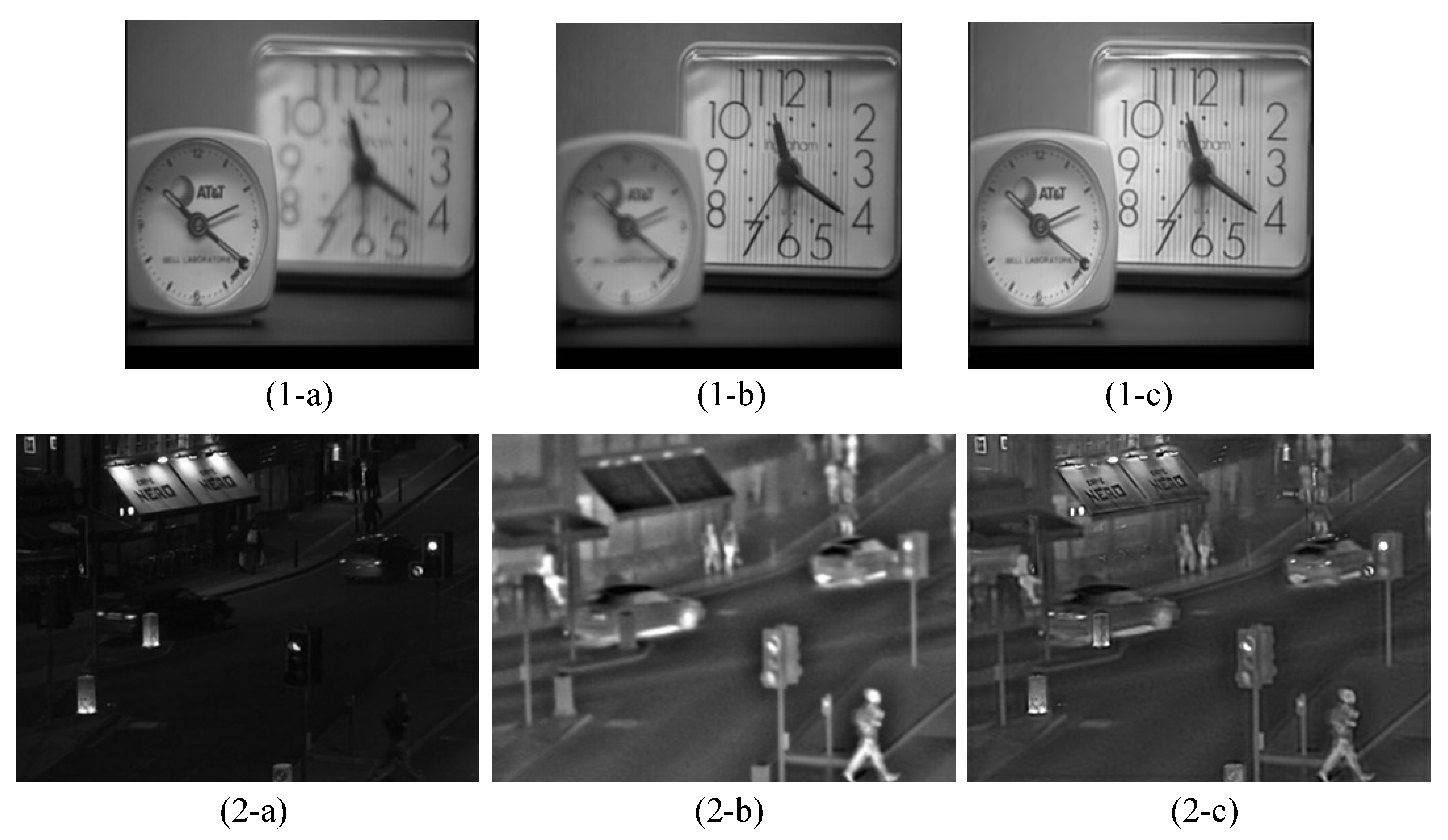
In order to show the potentiality of the proposed method in other applications of image fusion, our proposed method is applied to regular multi-focus and infrared-visible image pairs. Figure 9a–c show the fused multi-focus images, and Figure 9d–f show the fused infrared-visible images. We pick one fused image from each fusion type to do the detailed analysis.
In Figure 10, (1-a) and (1-b) are the multi-focus source images. Each of them has a different out-of-focus clock. (1-c) is the fused image by our proposed solution. Two clocks are in focus in (1-c). Similarly, Figure 10 (2-a) and (2-b) are the infrared-visible source images. (2-a) as the visible image only reveals the visible details of background, such as lights and the storefront. (2-b) as the infrared image shows the people, vehicles, and other missing details in visible image (2-a). (2-c) as the fused image contains the background and detailed information of both (2-a) and (2-b). These experiments confirm that our proposed solution can generate the satisfactory fused image in multi-focus and infrared-visible scene.
5. Conclusions
This paper proposed a framework that integrated entropy-based clustering and online dictionary learning in a sparse representation process. Compared with traditional medical image fusion methods, the integrated approach had two major improvements. First, it used an L2-norm based weighted average method to fuse low-frequency components of a source image. Second, an online dictionary learning algorithm was used to extract discriminative features from high-frequency components of source that enhances the accuracy and efficiency of image fusion. The comparative experiments with BSD, DWT, DT-CWT, CS-DCT, KSVD-OMP, MFR, SRDL, JPC and MST-SR demonstrated that the proposed IDLE had a better performance than other methods in CT-MRI, MRI-PET and MRI-SPECT image fusion. However, the proposed IDLE used Gaussian filter to eliminate the high-frequency details of source image. A part of the high-frequency information cannot not be presented in the fused outcome. In future research, the proposed IDLE will improve the noise filtering without damaging the high-frequency information.
Acknowledgments
We would like to thank the supports by National Natural Science Foundation of China (NSFC) (51505054), Chongqing Municipal Education Commission (KJ1500405), Chongqing Science and Technology Commission (cstc2015zdcy-ztzx60002), Student Innovation Training Program of Chongqing University of Posts and Telecommunications (A2017-30), and Graduate Scientific Research Starting Foundation of Chongqing University of Posts and Telecommunications (A2017-13).
Author Contributions
Guanqiu Qi and Zhiqin Zhu conceived and designed the experiments; Jinchuan Wang, Qiong Zhang and Fancheng Zeng performed the experiments; Guanqiu Qi and Zhiqin Zhu analyzed the data; Zhiqin Zhu contributed reagents/materials/analysis tools; Guanqiu Qi and Zhiqin Zhu wrote the paper; Guanqiu Qi and Zhiqin Zhu provided technical support and revised the paper.
Conflicts of Interest
The authors declare no conflict of interest.
References
- Tsai, W.T.; Qi, G. DICB: Dynamic Intelligent Customizable Benign Pricing Strategy for Cloud Computing. In Proceedings of the 2012 IEEE Fifth International Conference on Cloud Computing (CLOUD), Honolulu, HI, USA, 24–29 June 2012; pp. 654–661. [Google Scholar]
- Tsai, W.T.; Qi, G.; Chen, Y. A Cost-Effective Intelligent Configuration Model in Cloud Computing. In Proceedings of the 2012 32nd International Conference on Distributed Computing Systems Workshops, Macau, China, 18–21 June 2012; pp. 400–408. [Google Scholar]
- Tsai, W.T.; Qi, G. Integrated fault detection and test algebra for combinatorial testing in TaaS (Testing-as-a-Service). Simulation Modelling Practice and Theory 2016, 68, 108–124. [Google Scholar] [CrossRef]
- Wikipedia, Magnetic Resonance Imaging. Available online: https://en.wikipedia.org/wiki/Magnetic_resonance_imaging (accessed on 1 October 2017).
- Wikipedia, Computed Tomography. Available online: https://en.wikipedia.org/wiki/CT_scan (accessed on 1 October 2017).
- RadiologyInfo, Positron Emission Tomography. Available online: https://www.radiologyinfo.org (accessed on 1 October 2017).
- Mayfield, Single Photon Emission Computed Tomography. Available online: https://www.mayfieldclinic.com/PE-SPECT.htm (accessed on 1 October 2017).
- May, K.A.; Georgeson, M.A. Blurred edges look faint, and faint edges look sharp: The effect of a gradient threshold in a multi-scale edge coding model. Vis. Res. 2007, 47, 1705–1720. [Google Scholar] [CrossRef] [PubMed]
- Zhu, Z.; Qi, G.; Chai, Y.; Yin, H.; Sun, J. A Novel Visible-infrared Image Fusion Framework for Smart City. Int. J. Simul. Process Model. 2016, (in press). [Google Scholar]
- Buades, A.; Coll, B.; Morel, J.M. Image denoising methods: A new nonlocal principle. SIAM Rev. 2010, 52, 113–147. [Google Scholar] [CrossRef]
- Vankawala, F.; Ganatra, A.; Patel, A. Article: A survey on different image deblurring techniques. Int. J. Comput. Appl. 2015, 116, 15–18. [Google Scholar]
- Bertalmio, M.; Sapiro, G.; Caselles, V.; Ballester, C. Image inpainting. In Proceedings of the 27th Annual Conference on Computer Graphics and Interactive Techniques, New Orleans, LA, USA, 23–28 July 2000. [Google Scholar]
- Glasner, D.; Bagon, S.; Irani, M. Super-resolution from a single image. In Proceedings of the 2009 International Conference on Computer Vision, Kyoto, Japan, 29 September–2 October 2009. [Google Scholar]
- Zhang, Y. Understanding image fusion. Photogramm. Eng. Remote Sens. 2004, 70, 657–661. [Google Scholar]
- Yang, B.; Li, S. Multifocus image fusion and restoration with sparse representation. IEEE Trans. Instrum. Meas. 2010, 59, 884–892. [Google Scholar] [CrossRef]
- Aharon, M.; Elad, M.; Bruckstein, A. K-SVD: An algorithm for designing overcomplete dictionaries for sparse representation. IEEE Trans. Signal Process. 2006, 54, 4311–4322. [Google Scholar] [CrossRef]
- Zhu, Z.; Sun, J.; Qi, G.; Chai, Y.; Chen, Y. Frequency Regulation of Power Systems with Self-Triggered Control under the Consideration of Communication Costs. Applied Sciences 2017, 7, 688. [Google Scholar] [CrossRef]
- Lee, H.; Battle, A.; Raina, R.; Ng, A.Y. Efficient sparse coding algorithms. In Proceedings of the 20th Annual Conference on Neural Information Processing Systems, Vancouver, BC, Canada, 4–7 December 2006. [Google Scholar]
- Mairal, J.; Bach, F.; Ponce, J.; Sapiro, G. Online learning for matrix factorization and sparse coding. J. Mach. Learn. Res. 2010, 11, 19–60. [Google Scholar]
- Qi, G.; Tsai, W.T.; Li, W.; Zhu, Z.; Luo, Y. A cloud-based triage log analysis and recovery framework. Simul. Model. Pract. Theory 2017, 77, 292–316. [Google Scholar] [CrossRef]
- Tsai, W.; Qi, G.; Zhu, Z. Scalable SaaS Indexing Algorithms with Automated Redundancy and Recovery Management. Int. J. Software Inform. 2013, 7, 63–84. [Google Scholar]
- Zhang, Q.; Fu, Y.; Li, H.; Zou, J. Dictionary learning method for joint sparse representation-based image fusion. Opt. Eng. 2013, 52. [Google Scholar] [CrossRef]
- Kim, M.; Han, D.K.; Ko, H. Joint patch clustering-based dictionary learning for multimodal image fusion. Inform. Fusion 2016, 27, 198–214. [Google Scholar] [CrossRef]
- Li, S.; Yin, H.; Fang, L. Group-sparse representation with dictionary learning for medical image denoising and fusion. IEEE Trans. Biomed. Eng. 2012, 59, 3450–3459. [Google Scholar] [CrossRef] [PubMed]
- Wu, W.; Tsai, W.T.; Jin, C.; Qi, G.; Luo, J. Test-Algebra Execution in a Cloud Environment. In Proceedings of the 2014 IEEE 8th International Symposium on Service Oriented System Engineering, Oxford, UK, 7–11 April 2014; pp. 59–69. [Google Scholar]
- Tsai, W.T.; Luo, J.; Qi, G.; Wu, W. Concurrent Test Algebra Execution with Combinatorial Testing. In Proceedings of the 2014 IEEE 8th International Symposium on Service Oriented System Engineering, Washington, DC, USA, 7–11 April 2014; pp. 35–46. [Google Scholar]
- Liu, Y.; Liu, S.; Wang, Z. A general framework for image fusion based on multi-scale transform and sparse representation. Inform. Fusion 2015, 24, 147–164. [Google Scholar] [CrossRef]
- Hyvärinen, A. Fast and robust fixed-point algorithms for independent component analysis. Neural Netw. IEEE Trans. 1999, 10, 626–634. [Google Scholar] [CrossRef] [PubMed]
- Zou, H.; Hastie, T.; Tibshirani, R. Sparse principal component analysis. J. Comput. Graph. Stat. 2006, 15, 265–286. [Google Scholar] [CrossRef]
- Nikolakopoulos, K.G. Comparison of nine fusion techniques for very high resolution data. Photogramm. Eng. Remote Sens. 2008, 74, 647–659. [Google Scholar] [CrossRef]
- Li, X.; Li, H.; Yu, Z.; Kong, Y. Multifocus image fusion scheme based on the multiscale curvature in nonsubsampled contourlet transform domain. Opt. Eng. 2015, 54. [Google Scholar] [CrossRef]
- Yang, Y.; Tong, S.; Huang, S.; Lin, P. Dual-tree complex wavelet transform and image block residual-based multi-focus image fusion in visual sensor networks. Sensors 2014, 14, 22408–22430. [Google Scholar] [CrossRef] [PubMed]
- Lemeshewsky, G.P. Multispectral multisensor image fusion using wavelet transforms. In Proceedings of the SPIE—The International Society for Optical Engineering, Orlando, FL, USA, 6 April 1999. [Google Scholar]
- Al-Azzawi, N.; Sakim, H.A.M.; Abdullah, A.K.W.; Ibrahim, H. Medical image fusion scheme using complex contourlet transform based on PCA. In Proceedings of the 2009 31st Annual International Conference of the IEEE Engineering in Medicine and Biology Society (EMBC), Minneapolis, MN, USA, 3–6 September 2009. [Google Scholar]
- Chung, T.; Liu, Y.; Chen, C.; Sun, Y.; Chiu, N.; Lee, J. Intermodality registration and fusion of liver images for medical diagnosis. In Proceedings of the Intelligent Information Systems, IIS’97, Grand Bahama Island, Bahamas, 8–10 December 1997. [Google Scholar]
- Phegley, J.; Perkins, K.; Gupta, L.; Dorsey, J.K. Risk-factor fusion for predicting multifactorial diseases. Biomed. Eng. IEEE Trans. 2002, 49, 72–76. [Google Scholar] [CrossRef] [PubMed]
- Zhang, Z.M.; Yao, J.; Bajwa, S.; Gudas, T. “Automatic” multimodal medical image fusion. In Proceedings of the 2003 IEEE International Workshop on Soft Computing in Industrial Applications, Provo, UT, USA, 17 May 2003. [Google Scholar]
- Zhu, Z.; Yin, H.; Chai, Y.; Li, Y.; Qi, G. A novel multi-modality image fusion method based on image decomposition and sparse representation. Inform. Sci. 2017, in press. [Google Scholar] [CrossRef]
- Olshausen, B.; Field, D. Emergence of simple-cell receptive field properties by learning a sparse code for natural images. Nature 1996, 381, 607–609. [Google Scholar] [CrossRef] [PubMed]
- Huang, K.; Aviyente, S. Sparse representation for signal classification. In Proceedings of the 20th Annual Conference on Neural Information Processing Systems, Vancouver, BC, Canada, 4–7 December 2006. [Google Scholar]
- Husoy, J.H.; Engan, K.; Aase, S. Method of optimal directions for frame design. In Proceedings of the 1999 IEEE International Conference on Acoustics, Speech, and Signal Processing, Phoenix, AZ, USA, 15–19 March 1999. [Google Scholar]
- Rubinstein, R.; Zibulevsky, M.; Elad, M. Double sparsity: Learning sparse dictionaries for sparse signal approximation. IEEE Trans. Signal Process. 2010, 58, 1553–1564. [Google Scholar] [CrossRef]
- Yang, B.; Li, S. Pixel-level image fusion with simultaneous orthogonal matching pursuit. Inform. Fusion 2012, 13, 10–19. [Google Scholar] [CrossRef]
- Nejati, M.; Samavi, S.; Shirani, S. Multi-focus image fusion using dictionary-based sparse representation. Inform. Fusion 2015, 25, 72–84. [Google Scholar] [CrossRef]
- Dong, W.; Li, X.; Zhang, D.; Shi, G. Sparsity-based image denoising via dictionary learning and structural clustering. In Proceedings of the 2011 IEEE International Conference on Computer Vision and Pattern Recognition (CVPR), Colorado Springs, CO, USA, 20–25 June 2011. [Google Scholar]
- Chatterjee, P.; Milanfar, P. Clustering-based denoising with locally learned dictionaries. Trans. Image Process. 2009, 18, 1438–1451. [Google Scholar] [CrossRef] [PubMed]
- Mairal, J. Stochastic majorization-minimization algorithms for large-scale optimization. In Advances in Neural Information Processing Systems 26; Burges, C., Bottou, L., Welling, M., Ghahramani, Z., Weinberger, K., Eds.; Neural Information Processing Systems Foundation: Brussels, Belgium, 2013; pp. 2283–2291. [Google Scholar]
- Zhu, Z.; Qi, G.; Chai, Y.; Chen, Y. A Novel Multi-Focus Image Fusion Method Based on Stochastic Coordinate Coding and Local Density Peaks Clustering. Future Internet 2016, 8, 53. [Google Scholar] [CrossRef]
- Qiu, Q.; Jiang, Z.; Chellappa, R. Sparse dictionary-based representation and recognition of action attributes. In Proceedings of the 2011 IEEE International Conference on Computer Vision (ICCV), Barcelona, Spain, 6–13 November 2011. [Google Scholar]
- Siyahjani, F.; Doretto, G. Learning a Context Aware Dictionary for Sparse Representation; Lecture Notes in Computer Science Book Series; Springer: Berlin/Heidelberg, Germany, 2013; pp. 228–241. [Google Scholar]
- Kong, S.; Wang, D. A dictionary learning approach for classification: Separating the particularity and the commonality. In Proceedings of the 12th European Conference on Computer Vision, Florence, Italy, 7–13 October 2012. [Google Scholar]
- Yang, M.; Zhang, L.; Feng, X.; Zhang, D. Fisher discrimination dictionary learning for sparse representation. In Proceedings of the 2011 IEEE International Conference on Computer Vision (ICCV), Barcelona, Spain, 6–13 November 2011. [Google Scholar]
- Zhang, Q.; Li, B. Discriminative K-SVD for dictionary learning in face recognition. In Proceedings of the 2010 IEEE Conference on Computer Vision and Pattern Recognition (CVPR), San Francisco, CA, USA, 13–18 June 2010. [Google Scholar]
- James, M.L.; Gambhir, S.S. A molecular imaging primer: Modalities, imaging agents, and applications. Physiol. Rev. 2012, 92, 897–965. [Google Scholar] [CrossRef] [PubMed]
- Dong, J.; Zhuang, D.; Huang, Y.; Fu, J. Advances in multi-sensor data fusion: Algorithms and applications. Sensors 2009, 9, 7771–7784. [Google Scholar] [CrossRef] [PubMed]
- Okada, T.; Linguraru, M.G.; Hori, M.; Suzuki, Y.; Summers, R.M.; Tomiyama, N.; Sato, Y. Multi-organ segmentation in abdominal CT images. Conf. Proc. IEEE Eng. Med. Biol. Soc. 2012, 2012, 3986–3989. [Google Scholar] [PubMed]
- Lindeberg, T. Scale-space theory: A basic tool for analysing structures at different scales. J. Appl. Stat. 1994, 21, 225–270. [Google Scholar] [CrossRef]
- Wang, K.; Qi, G.; Zhu, Z.; Chai, Y. A Novel Geometric Dictionary Construction Approach for Sparse Representation Based Image Fusion. Entropy 2017, 19, 306. [Google Scholar] [CrossRef]
- Zhu, Z.; Qi, G.; Chai, Y.; Li, P. A Geometric Dictionary Learning Based Approach for Fluorescence Spectroscopy Image Fusion. Applied Sciences 2017, 7, 161. [Google Scholar] [CrossRef]
- Buades, A.; Coll, B.; Morel, J.M. On iMage Denoising Methods; Technical Report, Technical Note; Centre de Mathematiques et de Leurs Applications (CMLA): Paris, France, 2004. [Google Scholar]
- Wikipedia, Gaussian Blur. Available online: https://en.wikipedia.org/wiki/Gaussian_blur (accessed on 1 October 2017).
- Aharon, M.; Elad, M. Sparse and redundant modeling of image content using an image-signature-dictionary. SIAM J. Imaging Sci. 2008, 1, 228–247. [Google Scholar] [CrossRef]
- Zuo, Q.; Xie, M.; Qi, G.; Zhu, H. Tenant-based access control model for multi-tenancy and sub-tenancy architecture in Software-as-a-Service. Front. Comput. Sci. 2017, 11, 465–484. [Google Scholar] [CrossRef]
- Tsai, W.T.; Qi, G. Integrated Adaptive Reasoning Testing Framework with Automated Fault Detection. In Proceedings of the 2015 IEEE Symposium on Service-Oriented System Engineering, Redwood City, CA, USA, 30 March–3 April 2015; pp. 169–178. [Google Scholar]
- Li, S.; Kang, X.; Fang, L.; Hu, J.; Yin, H. Pixel-level image fusion: A survey of the state of the art. Inform. Fusion 2017, 33, 100–112. [Google Scholar] [CrossRef]
- Liu, Z.; Chai, Y.; Yin, H.; Zhou, J.; Zhu, Z. A novel multi-focus image fusion approach based on image decomposition. Inform. Fusion 2016, 35, 102–116. [Google Scholar] [CrossRef]
- Wu, Y.; Vansteenberge, J.; Mukunoki, M.; Minoh, M. Collaborative representation for classification, sparse or non-sparse? CoRR 2014, arXiv:1403.1353. [Google Scholar]
- Image Fusion Organization, Image Fusion Source Images. Available online: http://www.imagefusion.org (accessed on 20 October 2015).
- Johnson, K.A.; Becker, J.A. The Whole Brain Atlas. Available online: www.med.harvard.edu/aanlib/home.html (accessed on 17 June 2016).
- Hwang, B.M.; Lee, S.; Lim, W.T.; Ahn, C.B.; Son, J.H.; Park, H. A fast spatial-domain terahertz imaging using block-based compressed sensing. J. Infrared Millim. Terahertz Waves 2011, 32, 1328–1336. [Google Scholar] [CrossRef]
- Zheng, Y.; Essock, E.A.; Hansen, B.C.; Haun, A.M. A new metric based on extended spatial frequency and its application to DWT based fusion algorithms. Inform. Fusion 2007, 8, 177–192. [Google Scholar] [CrossRef]
- Anantrasirichai, N.; Achim, A.; Bull, D.; Kingsbury, N. Mitigating the effects of atmospheric distortion using DT-CWT fusion. In Proceedings of the 19th IEEE International Conference on Image Processing (ICIP), Orlando, FL, USA, 30 September–3 October 2012. [Google Scholar]
- Liu, Z.; Yin, H.; Chai, Y.; Yang, S.X. A novel approach for multimodal medical image fusion. Expert Syst. Appl. 2014, 41, 7425–7435. [Google Scholar] [CrossRef]
- Chen, H.; Huang, Z. Medical Image feature extraction and fusion algorithm based on K-SVD. In Proceedings of the 9th IEEE International Conference on P2P, Parallel, Grid, Cloud and Internet Computing (3PGCIC), Guangdong, China, 8–10 November 2014. [Google Scholar]
- Kumar, U.; Dasgupta, A.; Mukhopadhyay, C.; Joshi, N.; Ramachandra, T. Comparison of 10 multi-sensor image fusion paradigms for IKONOS images. Int. J. Res. Rev. Comput. Sci. 2011, 2, 40–47. [Google Scholar]
- Dixon, T.D.; Canga, E.F.; Nikolov, S.G.; Troscianko, T.; Noyes, J.M.; Canagarajah, C.N.; Bull, D.R. Selection of image fusion quality measures: Objective, subjective, and metric assessment. J. Opt. Soc. Am. A 2007, 24, B125–B135. [Google Scholar] [CrossRef]
- Qu, G.; Zhang, D.; Yan, P. Information measure for performance of image fusion. Electron. Lett. 2002, 38, 313–315. [Google Scholar] [CrossRef]
- Xydeas, C.; Petrović, V. Objective image fusion performance measure. Electron. Lett. 2000, 36, 308–309. [Google Scholar] [CrossRef]
- Sheikh, H.; Bovik, A. Image information and visual quality. IEEE Trans. Image Process. 2006, 15, 430–444. [Google Scholar] [CrossRef] [PubMed]
- Manchanda, M.; Sharma, R. A novel method of multimodal medical image fusion using fuzzy transform. J. Vis. Commun. Image Represent. 2016, 40, 197–217. [Google Scholar] [CrossRef]
- James, A.P.; Dasarathy, B.V. Medical image fusion: A survey of the state of the art. Inform. Fusion 2014, 19, 4–19. [Google Scholar] [CrossRef]
- Xu, X.; Shan, D.; Wang, G.; Jiang, X. Multimodal medical image fusion using PCNN optimized by the QPSO algorithm. Appl. Soft Comput. 2016, 46, 588–595. [Google Scholar] [CrossRef]
Figure 1.
The Proposed Image Fusion Framework.

Figure 2.
The Source Image Pair of Non-decomposition and Decomposition, (a) is the CT source image; and (b) is the MRI source image.
Figure 2.
The Source Image Pair of Non-decomposition and Decomposition, (a) is the CT source image; and (b) is the MRI source image.
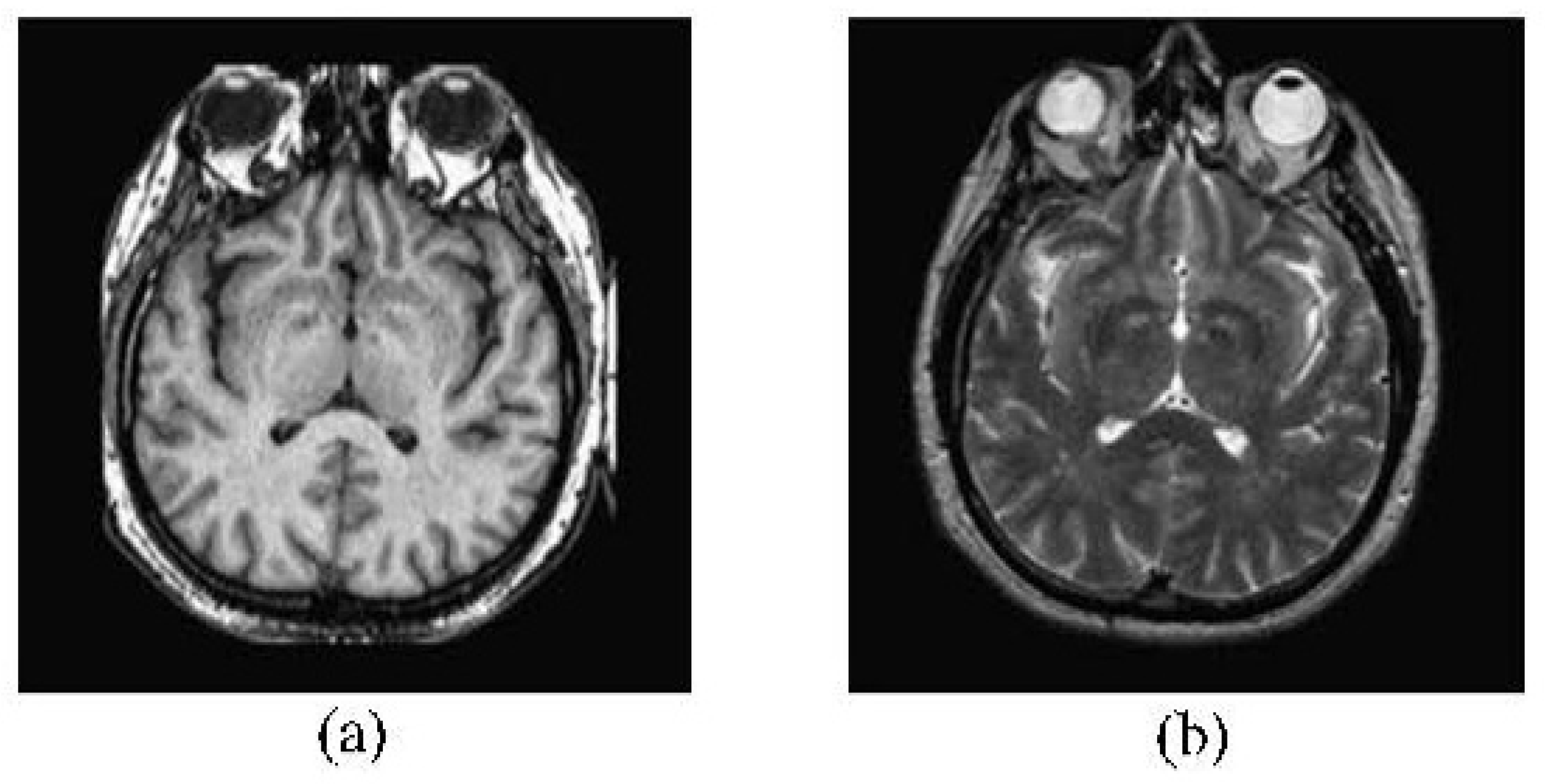
Figure 3.
Detailed Comparison of Non-decomposition and Decomposition, (a) is the fused result of non-decomposition; and (b) is the fused result of decomposition.
Figure 3.
Detailed Comparison of Non-decomposition and Decomposition, (a) is the fused result of non-decomposition; and (b) is the fused result of decomposition.

Figure 4.
Details Comparison of Learned Dictionary, (a) shows the details of a learned dictionary using traditional method; and (b) shows the details of a learned dictionary using proposed method.
Figure 4.
Details Comparison of Learned Dictionary, (a) shows the details of a learned dictionary using traditional method; and (b) shows the details of a learned dictionary using proposed method.

Figure 5.
Nine Image Fusion Comparative Experiments, (a)–(c) are CT-MRI source image pairs; (d)–(f) are MRI-PET source image pairs; and (g)–(i) are MRI-SPECT source image pairs.
Figure 5.
Nine Image Fusion Comparative Experiments, (a)–(c) are CT-MRI source image pairs; (d)–(f) are MRI-PET source image pairs; and (g)–(i) are MRI-SPECT source image pairs.
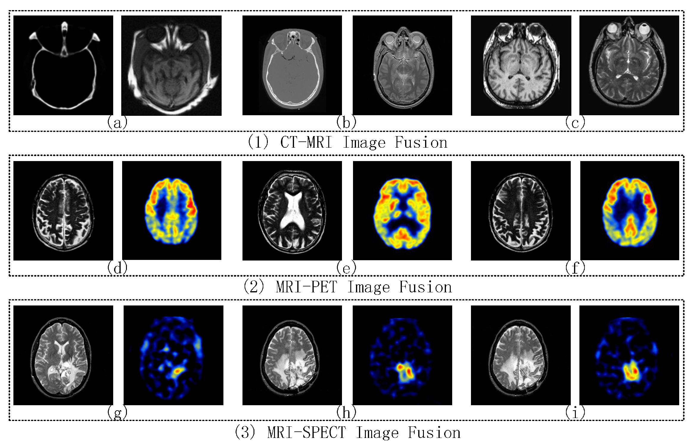
Figure 6.
CT-MRI Image Fusion Comparative Experiments, (a) is the CT source image; (b) is the MRI source image; and (c)–(l) are the fused images of BSD, DWT, DT-CWT, CS-DCT, KSVD-OMP, MFR, SRDL, JPC, MST-SR, and the proposed IDLE respectively.
Figure 6.
CT-MRI Image Fusion Comparative Experiments, (a) is the CT source image; (b) is the MRI source image; and (c)–(l) are the fused images of BSD, DWT, DT-CWT, CS-DCT, KSVD-OMP, MFR, SRDL, JPC, MST-SR, and the proposed IDLE respectively.
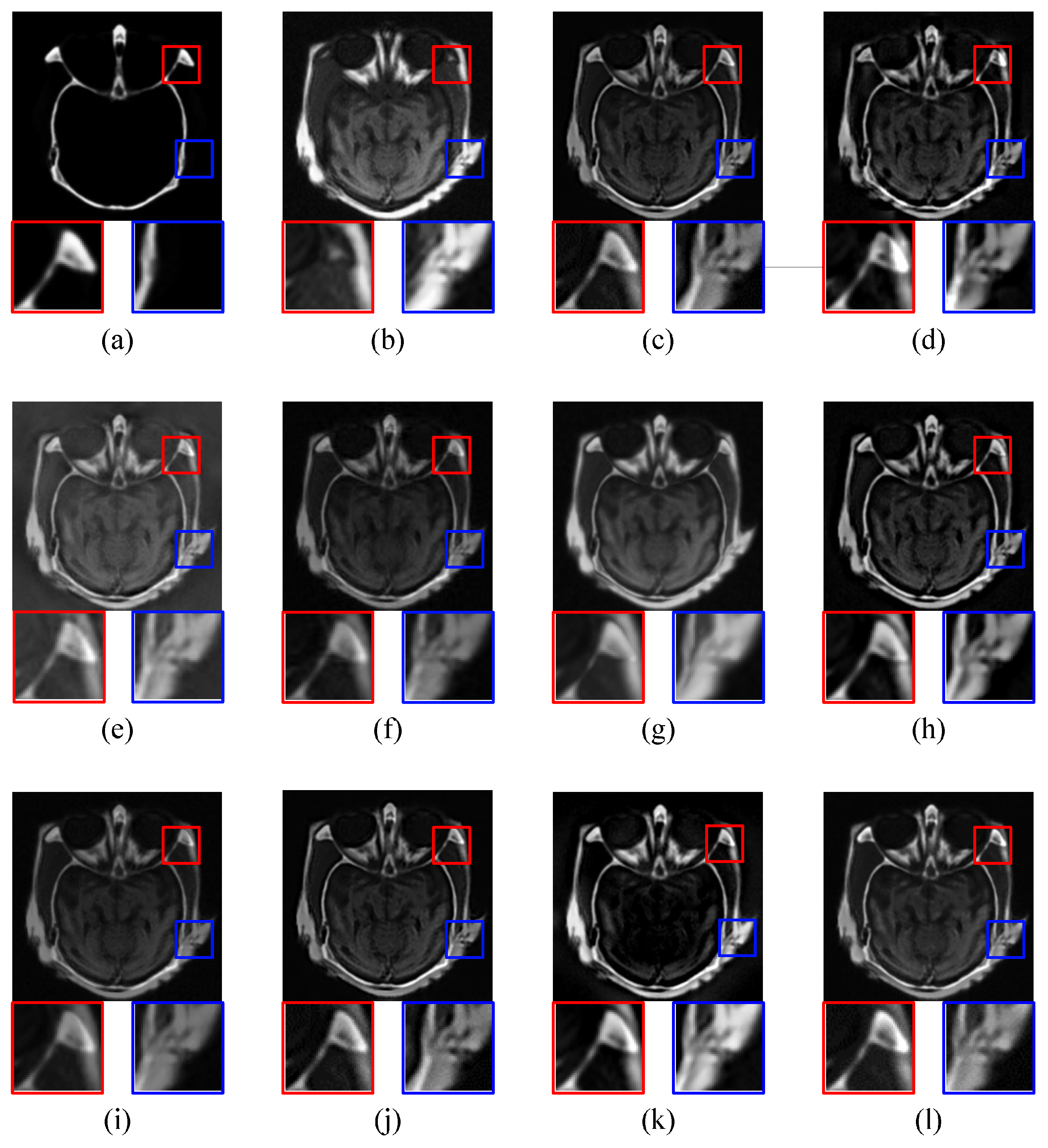
Figure 7.
MRI-PET Image Fusion Comparative Experiments, (a) is the MRI source image; (b) is the PET source image; and (c)–(l) are the fused images of BSD, DWT, DT-CWT, CS-DCT, KSVD-OMP, MFR, SRDL, JPC, MST-SR, and the proposed IDLE respectively.
Figure 7.
MRI-PET Image Fusion Comparative Experiments, (a) is the MRI source image; (b) is the PET source image; and (c)–(l) are the fused images of BSD, DWT, DT-CWT, CS-DCT, KSVD-OMP, MFR, SRDL, JPC, MST-SR, and the proposed IDLE respectively.

Figure 8.
MRI-SPECT Image Fusion Comparative Experiments, (a) is the MRI source image; (b) is the SPECT source image; and (c)–(l) are the fused images of BSD, DWT, DT-CWT, CS-DCT, KSVD-OMP, MFR, SRDL, JPC, MST-SR, and the proposed IDLE respectively.
Figure 8.
MRI-SPECT Image Fusion Comparative Experiments, (a) is the MRI source image; (b) is the SPECT source image; and (c)–(l) are the fused images of BSD, DWT, DT-CWT, CS-DCT, KSVD-OMP, MFR, SRDL, JPC, MST-SR, and the proposed IDLE respectively.
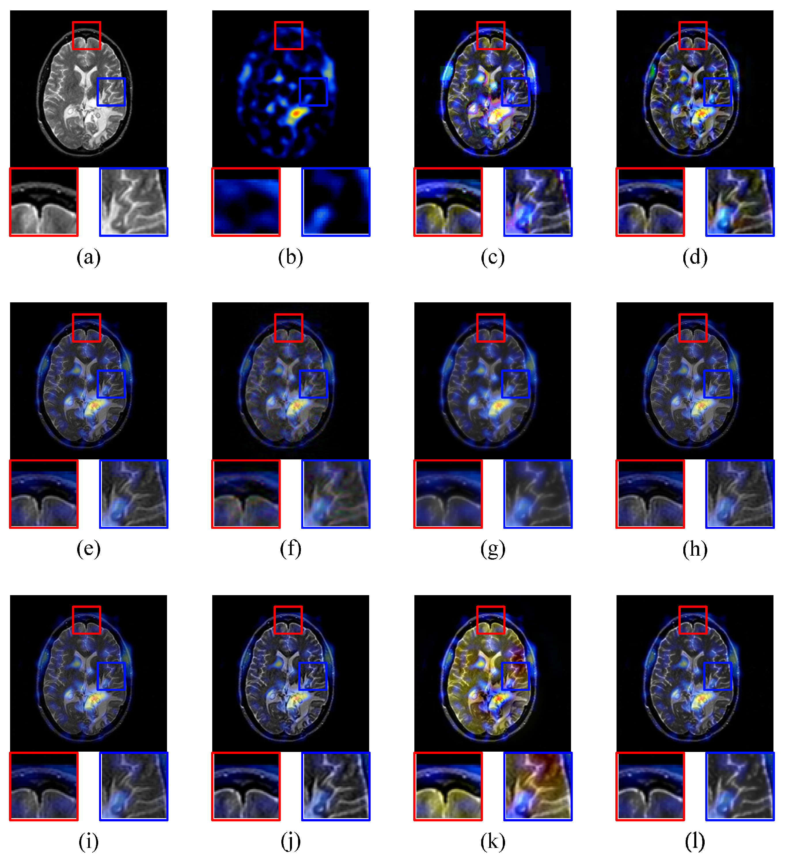
Figure 9.
Image Fusion Results of Proposed Solution in Different Scenes, (a)–(c) are the fused multi-focus images; and (d)–(f) are the fused infrared-visible images.
Figure 9.
Image Fusion Results of Proposed Solution in Different Scenes, (a)–(c) are the fused multi-focus images; and (d)–(f) are the fused infrared-visible images.
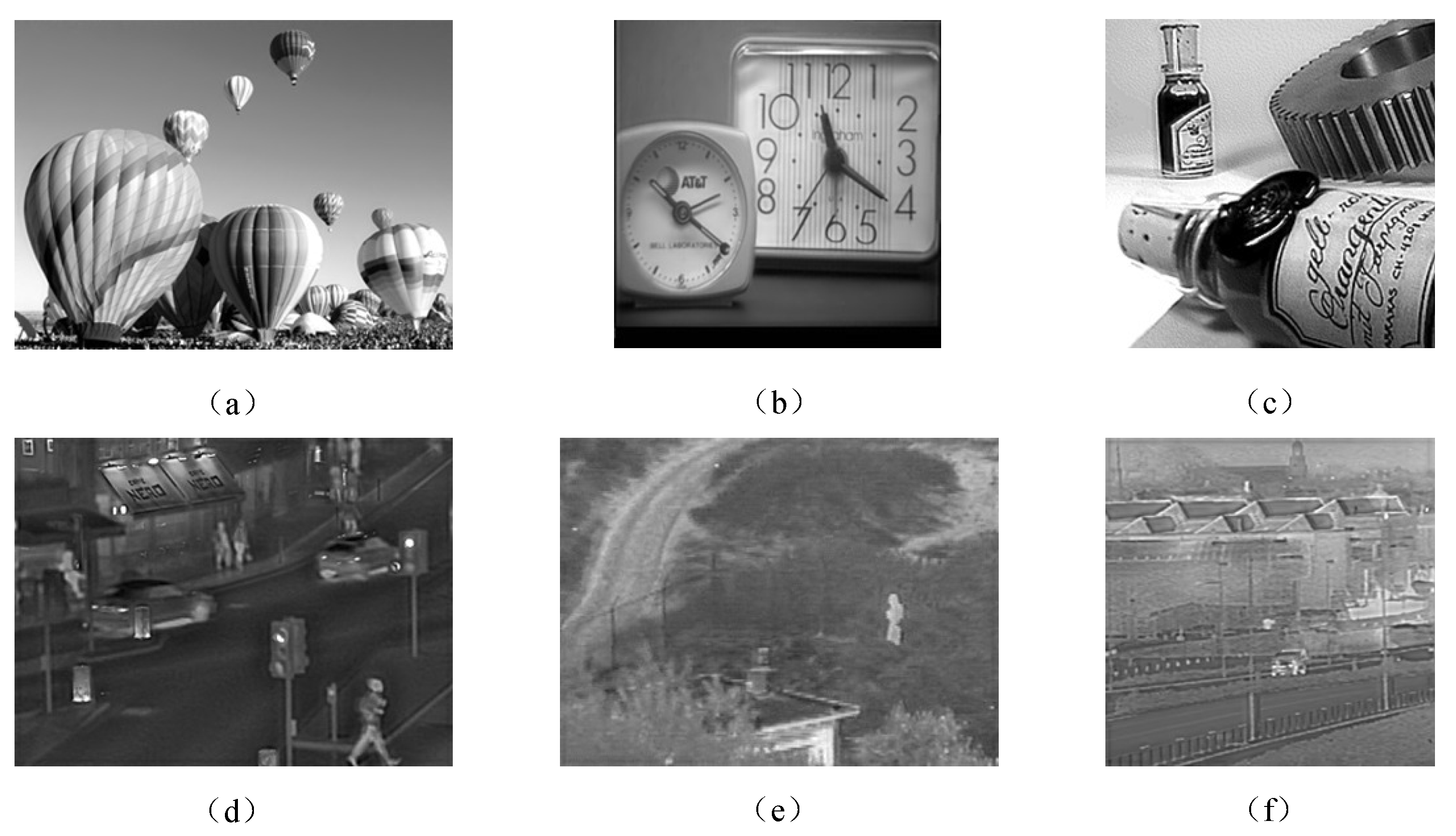
Figure 10.
Multi-focus and Infrared-visible Image Fusion Results of Proposed Solution, (1-a) and (1-b) are the multi-focus source images, (1-c) is the fused image by our proposed solution, (2-a) and (2-b) are the infrared-visible source images, and (2-c) is is the fused image by our proposed solution.


Table 1.
Objective Evaluations of CT-MRI Image Fusion Comparative Experiments.
| AG | EI | MI | VIF | ||
|---|---|---|---|---|---|
| BSD | 7.1738 | 76.9148 | 0.6595 | 2.1021 | 0.4021 |
| DWT | 6.1569 | 56.8719 | 0.6284 | 1.3327 | 0.2952 |
| DT-CWT | 4.2628 | 46.2560 | 0.5097 | 1.2463 | 0.2632 |
| CS-DCT | 3.5918 | 38.7132 | 0.5063 | 2.0268 | 0.3046 |
| KSVD-OMP | 4.2109 | 46.0699 | 0.7762 | 2.5085 | 0.3493 |
| MFR | 6.0671 | 62.1495 | 0.7442 | 2.7284 | 0.3691 |
| SRDL | 4.6062 | 53.2307 | 0.7238 | 2.6084 | 0.3417 |
| JPC | 6.1482 | 64.5306 | 0.7264 | 2.5146 | 0.3908 |
| MST-SR | 4.4807 | 49.1622 | 0.6843 | 2.4708 | 0.3261 |
| Proposed IDLE | 6.1330 | 65.6209 | 0.8428 | 3.0158 | 0.4097 |
* The highest result of each objective metric is marked in bold-face.
Table 2.
Objective Evaluations of MRI-PET Image Fusion Comparative Experiments.
| AG | EI | MI | VIF | ||
|---|---|---|---|---|---|
| BSD | 6.7133 | 69.2493 | 0.3069 | 1.8505 | 0.2611 |
| DWT | 6.8695 | 70.8721 | 0.3128 | 1.7715 | 0.2447 |
| DT-CWT | 4.9488 | 47.1991 | 0.3147 | 1.8667 | 0.2954 |
| CS-DCT | 4.1109 | 42.9211 | 0.2955 | 1.8330 | 0.2694 |
| KSVD-OMP | 3.5764 | 36.7095 | 0.2840 | 1.7970 | 0.2842 |
| MFR | 4.9026 | 47.9372 | 0.3155 | 1.8673 | 0.3096 |
| SRDL | 5.0374 | 49.1628 | 0.3163 | 1.8571 | 0.3142 |
| JPC | 4.6936 | 47.6084 | 0.3184 | 1.8647 | 0.3086 |
| MST-SR | 3.7241 | 38.9104 | 0.2894 | 1.8163 | 0.2907 |
| Proposed IDLE | 4.7137 | 48.0413 | 0.3199 | 1.8744 | 0.3161 |
* The highest result of each objective metric is marked in bold-face.
Table 3.
Objective Evaluations of MRI-SPECT Image Fusion Comparative Experiments.
| AG | EI | MI | VIF | ||
|---|---|---|---|---|---|
| BSD | 5.8505 | 59.7385 | 0.7180 | 1.5139 | 0.2951 |
| DWT | 4.6099 | 57.2050 | 0.6397 | 1.3106 | 0.2766 |
| DT-CWT | 3.8157 | 37.3078 | 0.7079 | 1.6847 | 0.3212 |
| CS-DCT | 3.0988 | 31.6784 | 0.3601 | 1.4818 | 0.2695 |
| KSVD-OMP | 2.7215 | 38.1780 | 0.6497 | 1.6565 | 0.2898 |
| MFR | 4.5781 | 51.8703 | 0.7174 | 1.7067 | 0.3196 |
| SRDL | 4.8603 | 51.3517 | 0.7219 | 1.6973 | 0.3244 |
| JPC | 4.7361 | 52.5702 | 0.7196 | 1.7102 | 0.3227 |
| MST-SR | 3.8729 | 43.7209 | 0.6173 | 1.5927 | 0.2681 |
| Proposed IDLE | 4.7295 | 52.0081 | 0.7317 | 1.7192 | 0.3265 |
* The highest result of each objective metric is marked in bold-face.
Table 4.
Average Objective Evaluations of Nine Image Fusion Comparative Experiments.
| AG | EI | MI | VIF | ||
|---|---|---|---|---|---|
| BSD | 5.5369 | 56.6304 | 0.3293 | 1.8758 | 0.2837 |
| DWT | 5.4205 | 55.1206 | 0.3585 | 1.2852 | 0.2471 |
| DT-CWT | 4.4082 | 45.0176 | 0.4376 | 1.6371 | 0.2847 |
| CS-DCT | 3.6498 | 36.8703 | 0.3974 | 1.8496 | 0.2745 |
| KSVD-OMP | 3.6265 | 39.9752 | 0.5382 | 1.8416 | 0.2984 |
| MFR | 5.1247 | 52.1774 | 0.5653 | 2.0934 | 0.3204 |
| SRDL | 4.9845 | 5.1983 | 0.5537 | 1.9416 | 0.3279 |
| JPC | 5.2903 | 55.0743 | 0.6149 | 1.9773 | 0.3395 |
| MST-SR | 4.0817 | 44.1942 | 0.5142 | 1.9237 | 0.3076 |
| Proposed IDLE | 5.2374 | 53.9238 | 0.6291 | 2.1045 | 0.3426 |
* The highest result of each objective metric is marked in bold-face.
© 2017 by the authors. Licensee MDPI, Basel, Switzerland. This article is an open access article distributed under the terms and conditions of the Creative Commons Attribution (CC BY) license (http://creativecommons.org/licenses/by/4.0/).
Share and Cite
MDPI and ACS Style
Qi, G.; Wang, J.; Zhang, Q.; Zeng, F.; Zhu, Z. An Integrated Dictionary-Learning Entropy-Based Medical Image Fusion Framework. Future Internet 2017, 9, 61. https://doi.org/10.3390/fi9040061
AMA Style
Qi G, Wang J, Zhang Q, Zeng F, Zhu Z. An Integrated Dictionary-Learning Entropy-Based Medical Image Fusion Framework. Future Internet. 2017; 9(4):61. https://doi.org/10.3390/fi9040061
Chicago/Turabian StyleQi, Guanqiu, Jinchuan Wang, Qiong Zhang, Fancheng Zeng, and Zhiqin Zhu. 2017. "An Integrated Dictionary-Learning Entropy-Based Medical Image Fusion Framework" Future Internet 9, no. 4: 61. https://doi.org/10.3390/fi9040061
Note that from the first issue of 2016, this journal uses article numbers instead of page numbers. See further details here.