Optimal Scheduling of Integrated Energy System Considering Electric Vehicle Battery Swapping Station and Multiple Uncertainties

Abstract

In recent years, there has been rapid advancement in new energy technologies aimed at mitigating greenhouse gas emissions stemming from fossil fuels. Nonetheless, uncertainties persist in both the power output of new energy sources and load. To effectively harness the economic and operational potential of an Integrated Energy System (IES), this paper introduces an enhanced uncertainty set. This set incorporates N-1 contingency considerations and the nuances of source–load distribution. This framework is applied to a robust optimization model for an Electric Vehicle Integrated Energy System (EV-IES), which includes Electric Vehicle Battery Swapping Station (EVBSS). Firstly, this paper establishes an IES model of the EVBSS, and then proceeds to classifies and schedules the large-scale battery groups within these stations. Secondly, this paper proposes an enhanced uncertainty set to account for the operational status of multiple units in the system. It also considers the output characteristics of both new energy sources and loads. Additionally, it takes into consideration the N-1 contingency state and multi-interval distribution characteristics. Subsequently, a multi-time-scale optimal scheduling model is established with the objective of minimizing the total cost of the IES. The day-ahead robust optimization fully considers the multivariate uncertainty of the IES. The solution employs the Nested Column and Constraint Generation (C&CG) algorithm, based on the distribution characteristics of multiple discrete variables in the model. The intraday optimal scheduling reallocates the power of each unit based on the robust optimization results from the day-ahead scheduling. Finally, the simulation results demonstrate that the proposed method effectively reduces the conservatism of the uncertainty set, ensuring economic and stable operation of the EV-IES while meeting the demands of electric vehicle users.

1. Introduction

The IES with diversified energy supply and flexible operation mode, has attracted widespread attention both domestically and internationally due to its ability to alleviate the environmental pollution and energy shortages caused by traditional fossil fuels [1,2]. IESs complement, convert, and absorb various forms of energy. They provide a new approach to adjusting the energy structure, increasing the utilization of new energy, and reducing ecological pollution [3]. This represents a significant step towards achieving dual carbon goals and promoting green energy transformation [4].

EVs are widely embraced by the market for their advantages of low carbon emissions, high efficiency, and low maintenance costs [5,6]. However, constraints still exist regarding the widespread adoption of large-scale EV travel and charging infrastructure, such as limited driving range [7], unpredictable charging times [8], high battery degradation costs [9], and inadequate charging facilities [10]. Methods for supplementing electric energy for EVs include charging and battery swapping [11], with the latter being considered a potential solution to address the aforementioned drawbacks due to its advantages of short time consumption and high flexibility. Ref. [12] fully utilized retired batteries to reduce the purchasing costs of energy storage systems. It proposed battery charging and discharging control strategies, including fast charging, slow charging, and reverse output, based on load levels, effectively achieving peak load transfers within the grid. Ref. [13] incorporated energy prices and electrified traffic loads into the battery swapping station management system. It optimized the management of grid-to-vehicle and vehicle-to-grid interactions through predictive, real-time, and auxiliary services. However, the large-scale battery groups in battery swapping stations would render the battery scheduling model overly complex. Within the framework of the Energy Internet, integrating the EVBSS into the IES not only meets the evolving needs of EV users but also fully leverages the energy storage capabilities of large-scale battery groups, enhances the integration of new energy sources, and further explores the scheduling potential of EV-IES [14,15].

Accurately predicting natural conditions is extremely challenging, which implies fluctuations in the output of new energy. Moreover, the load within the power system is often complex and variable [16], resulting in the failure of real-time matching between the power output of new energy and the system load in the IES. Scholarly research has extensively addressed the scheduling issues of IES with uncertainty, where robust optimization emerges as an effective method to address this problem [17,18]. Ref. [19] established a two-layer optimization model for IES incorporating multiple types of energy storage. The upper layer aimed to minimize the cost of the energy storage system, while the lower layer aimed to minimize the operating cost of the IES. The influence of time on wind power output is introduced, and the Karush–Kuhn–Tucker (KKT) condition is used to solve the robust model. Ref. [2] proposed a framework for an IES coupled with biogas, solar energy, and wind energy. It employed a boxed uncertainty set to describe the fluctuation of uncertain variables introducing diversified evaluation indexes, and verified that the proposed method can ensure the stable operation of IES under worst-case scenarios. Ref. [20] introduced a new hybrid robust interval optimization (HRIO) strategy and utilized min–max robust techniques to transform the uncertainty constraints of the new energy output into deterministic constraints, allowing for more flexible adjustment of the optimization scheme. Ref. [21] utilized an uncertainty scenario simplification method, substituting fewer typical scenarios for the original scenarios. It employed a boxed uncertainty set model and optimal robust scheduling intervals to depict the uncertainty in new energy output. Finally, it combined the new energy–energy storage system with a value assessment method to demonstrate that grid connection of new energy introduced power fluctuations into the system, while energy storage equipment can mitigate the degree of fluctuation and enhance system revenue. Although the aforementioned literature integrates the system based on robust optimization, they fail to fully consider the distribution characteristics of uncertain variables. Furthermore, most of them are conducted under normal operation of the IES. If the discrete uncertainty of each unit is further considered, the system may operate in a special mode [22]. In actual operation, the operational metrics under special modes significantly differ from those in normal modes [23], thus various resources with coupling and scheduling plans in different states should be considered separately (see

Table 1. Comparison with several related references.

Refs.	Coupling Resources	Battery Model	Uncertainty Element	Robust Solution Algorithm
[2]	Wind, solar, biogas	---	Wind, solar, electric load, heat load, cold load	C&CG
[11]	---	EV charging station and battery swapping station, battery fast charging model	---	---
[12]	---	Battery charging process, battery discharging process, charging and discharging power regulation model	---	---
[13]	---	Battery charging process, battery discharging process, energy price incentive model	---	---
[14]	Solar, EV-IES	Battery charging process, battery discharging process	---	---
[15]	Wind, solar, natural gas, EVBSS	Battery charging process, battery discharging process	Wind, solar	---
[16]	Wind, solar	---	Wind, solar, electric load, heat load	C&CG
[17]	Wind, solar, natural gas	---	Wind, solar	KKT
[18]	Wind, gas	---	Wind	KKT
[19]	Wind, solar, natural gas	---	Wind, solar	KKT, HRIO
[20]	Wind, solar	---	Wind, solar	C&CG
[21]	---	---	N-1 contingency	---
This paper	Wind, solar, natural gas, EVBSS	Battery charging process, battery discharging process, charging and discharging priority function	Wind, solar, electric load, heat load, cold load, N-1 contingency	Nested C&CG

).

Based on the above background, existing IES should incorporate and consider EV loads to fully utilize the energy storage of large-scale battery populations. Meanwhile, current research fails to fully consider the spatial and temporal characteristics of uncertain variables, causing a conservative tendency in scheduling plans. To address these issues, this paper conducts an in-depth study of EV-IES planning combined with EV battery exchange services. Additionally, it explores how to improve operational scheduling of uncertainty aggregation in the N-1 fault state of the system. The main contributions of this study are as follows:

(1)

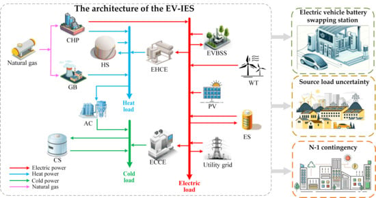
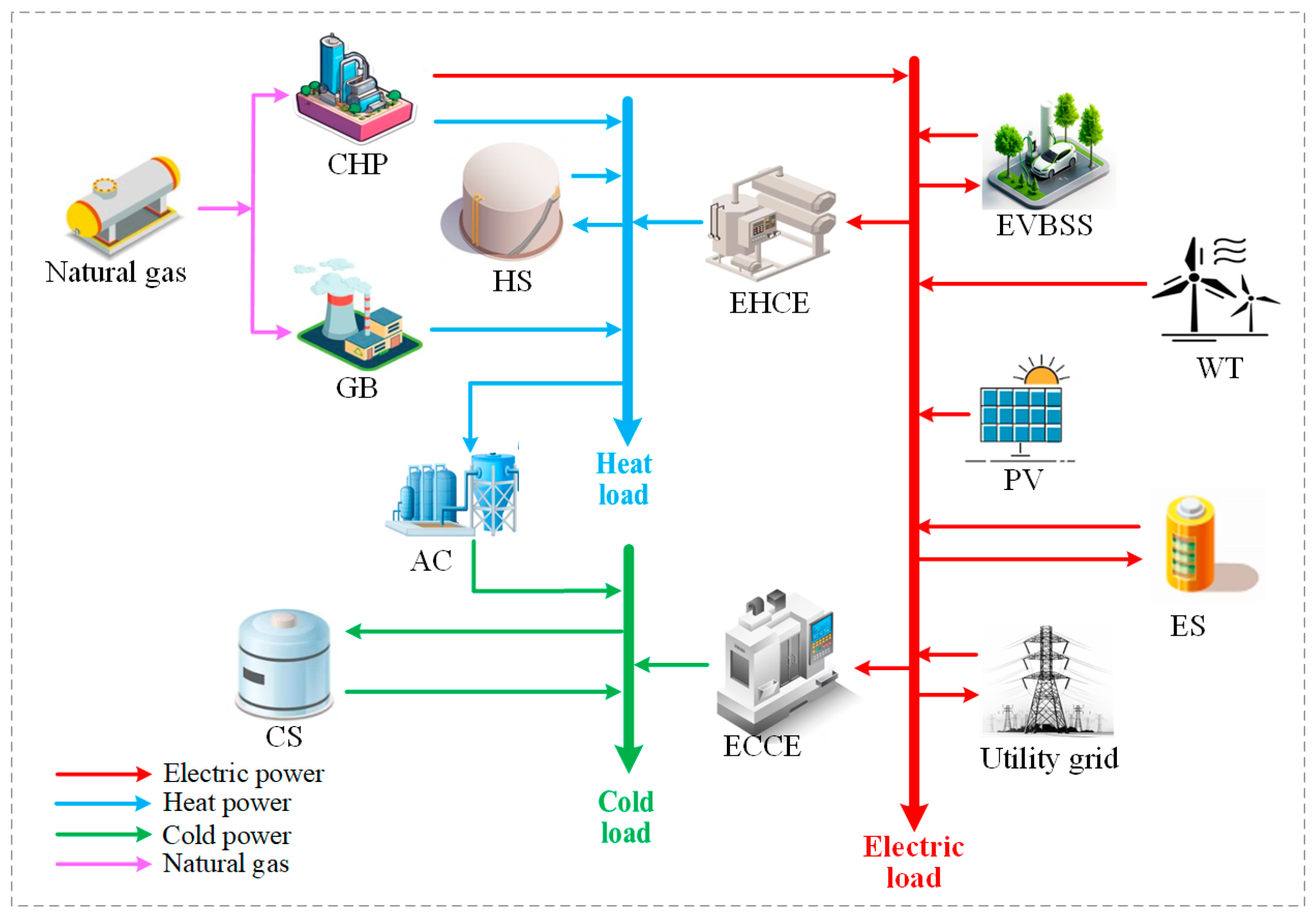
An EV-IES comprises electric power, heat power and cold power, encompassing various energy sources and devices. Furthermore, it considers the battery replacement needs of EV users.

(2)

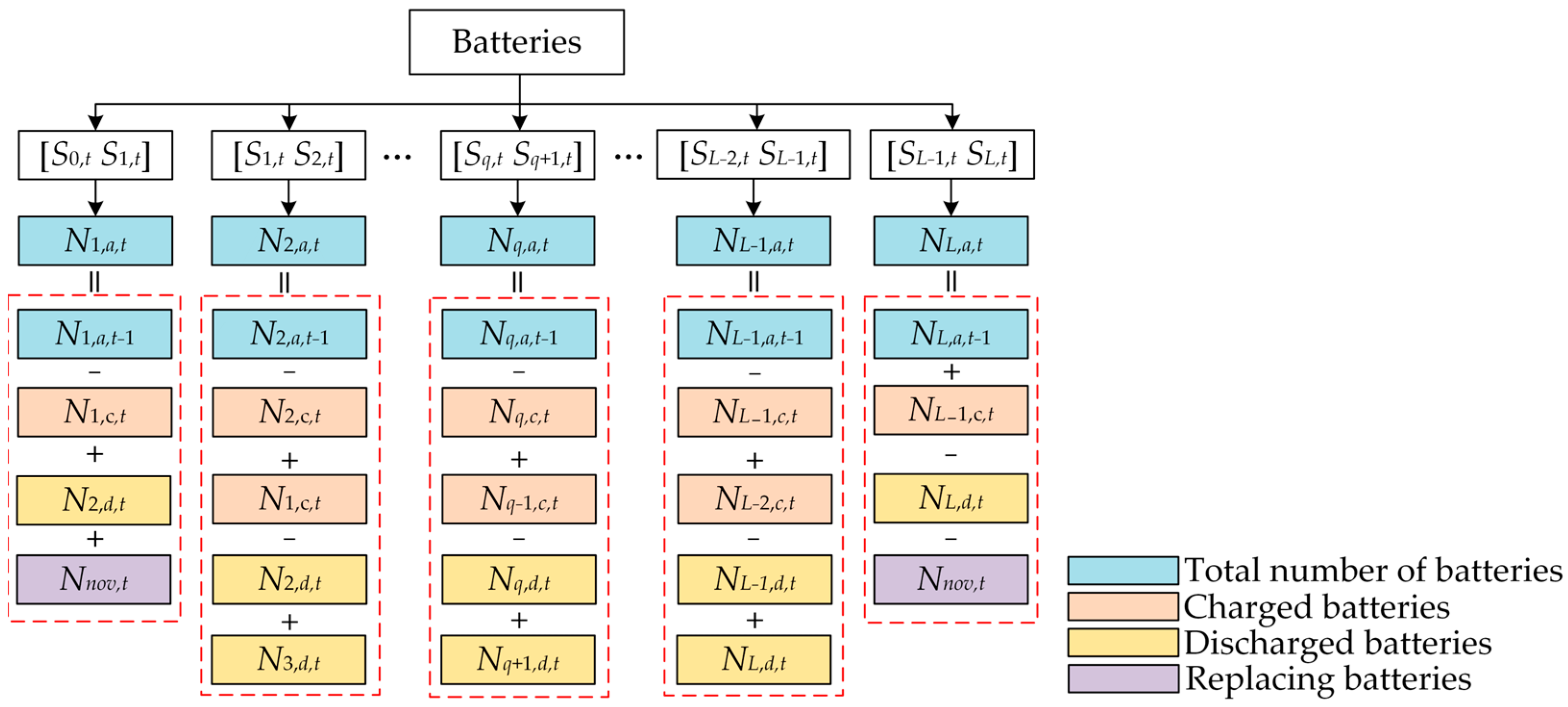
For the large-scale battery clustering in an EVBSS, a classification scheduling strategy based on battery State of Charge (SOC) is proposed, integrating a battery charging and discharging priority function.

(3)

Aiming at the new energy output characteristics, the study proposes an improved uncertainty ensemble with multi-interval distribution characteristics to reduce the conservatism of the traditional box uncertainty. In addition, the N-1 contingency uncertainty ensemble is proposed for the discrete operating states of multiple devices in the IES.

(4)

An EV-IES multi-time-scale optimal scheduling model is established. Day-ahead robust optimization fully considered the multiple uncertainties in the system. According to the distribution of binary discrete variables in the robust model, the nested C&CG algorithm was used to solve the mixed integer robust model. Intraday optimal scheduling is based on the day-before robust optimization results to reduce the power fluctuation caused by the deviation in the predicted source load.

The subsequent sections of this paper are organized as follows: Section 2 introduces the planning and mathematical modeling of EV-IES. Section 3 presents the EV-IES multi-time-scale optimization scheduling model with an improved uncertainty ensemble. Section 4 presents the numerical results of case studies. Finally, Section 5 offers concluding remarks.

2. EV-IES Model

EV-IES achieves efficient energy utilization through multi-energy coupling, including electricity, heat, and cold energy [24,25]. Its structure is shown in Figure 1.

The electric energy coupling equipment includes EVBSSs, Combined Heat and Power (CHP), Wind Turbine (WT), photovoltaic (PV) power generation equipment, electric energy storage (ES), utility grid, electricity–heat conversion equipment (EHCE), and electricity–cold conversion equipment (ECCE). The EVBSSs, ES, and the utility grid are able to input or output electrical power among them. The rest of the equipment can only achieve unidirectional power flow. Energy inputs include WT, PV, and grid purchase. The heat energy coupling equipment includes CHP, Heat Energy Storage (HS), Gas Boiler (GB), EHCE, and Absorption Chiller (AC). Among them, HS can realize the two-way heat power flow, and the other devices can only carry out one-way flow of thermal power. CHP and GBs require natural gas as fuel to generate power. The cold energy coupling equipment includes Cold Energy Storage (CS), AC, and ECCE. Only CS can absorb or release cold power. Energy outputs include electric load, heat load, and cold load.

2.1. Objective Function

The minimum operating cost of EV-IES is taken as the objective function. Its specific content is shown in Equation (1).

$$\begin{array}{l}\min {\displaystyle \sum _t(C_{uv}+C_{ps}+C_{mt})}\\ \left\{\begin{array}{l}{C}_{uv}=m_u^{CHP}{u}_t^{CHP}\\ C_{ps}=m_{gas}(G_t^{CHP}+G_t^{GB})+(m_b{P}_{b,t}-m_s{P}_{s,t})\Delta t\\ C_{mt}=[m^{CHP}{P}_t^{CHP}+m^{GB}{Q}_t^{GB}+m^{eh}{Q}_t^{eh}+m^{ec}{R}_t^{ec}+m^{ac}{R}_t^{ac}+\\ \hspace{1em}\hspace{1em} m^{es}(P_{c,t}^e+P_{d,t}^e)+m^{hs}(P_{c,t}^h+P_{d,t}^h)+m^{hc}(P_{c,t}^c+P_{d,t}^c)]\Delta t\end{array}\right.\end{array}$$

(1)

where C_uv, C_ps, and C_mt are equipment start-up cost, interaction cost, and maintenance cost, respectively. $m_u^{CHP}$ is the CHP start-up cost coefficient. M_gas, m_b, and m_s are the unit price of natural gas, the price of electricity purchased from the grid, and the price of electricity sold. m^CHP, m^GB, m^eh, m^ec, m^ac, m^es, m^hs, and m^hc are the maintenance cost coefficients of CHP, GB, EHCE and ECCE, AC, ES, HS, and CS systems, respectively. $u_t^{CHP}$ represents the start variable of the CHP device. P_b,t and P_s,t are the electricity purchased and sold in period t. $G_t^{CHP}$ and $G_t^{GB}$ represent the natural gas consumption of CHP and a GB, respectively. $P_t^{CHP}$, $Q_t^{GB}$, $Q_t^{eh}$, $R_t^{ec}$, $R_t^{ac}$, $P_{c,t}^e$, $P_{d,t}^e$, $P_{c,t}^h$, $P_{d,t}^h$, $P_{c,t}^c$, and $P_{d,t}^c$ represent the power of CHP, GB, EHCE, ECCE, ES, HS, CS systems, respectively.

2.2. EV Battery Swapping Station

In EVBSSs, due to the large scale of the battery group, decentralized scheduling needs a lot of time and computing power. So, this paper first divides it into L intervals according to the SOC of each battery in each period [26], and its structure is shown in Figure 2. In Figure 2, S_0,t represents the minimum SOC of the battery in the t period, S_L,t represents the maximum SOC of the battery in the t period, and the length of each interval is the same. N_q,a,t represents the total number of batteries in the q interval of the t period, q = 1,2, …, L. N_q,c,t and N_q,d,t represent the number of charged batteries and discharged batteries in the q interval, respectively. N_nov,t represents the number of EV users replacing batteries in the t period. Assuming that the operation period of IES is T, each interval can be subdivided into T intervals in a scheduling period, and the length of each interval is the same. When the EV arrives at the changing station, a battery in the [S_L−1,t S_L,t] interval is taken out for replacement, and the number of batteries in the interval will decrease, namely N_L,a,t = N_L,a,t−1. At the same time, the replaced batteries of the EV will be integrated into the [S_0,t S_1,t] interval, namely N_1,a,t = N_1,a,t+1. Because the SOC of the battery in the [S_L−1,t S_L,t] interval is high, these batteries can only be used for discharge scheduling or battery replacement services. The SOC of the battery in the [S_0,t S_1,t] interval is low. Only charging can be carried out, and discharging cannot be carried out. If N_nov,t EVs in the t period need to be replaced, N_1,a,t is the number of batteries in the t − 1 period plus the number of batteries replaced, minus the number of rechargeable batteries in the period, plus the number of discharged batteries in the [S_1,t S_2,t] interval. For batteries within the [S_L−1,t S_L,t] interval, N_L,a,t is the number of batteries in the t − 1 period minus the number of replacement batteries, plus the number of rechargeable batteries in the [S_L−2,t S_L−1,t] period, minus the number of discharged batteries in the period. For the batteries in the [S_q,t S_q+1,t] interval, it is not necessary to consider the number of battery replacements for EVs and rather only the number of charging and discharging batteries in the adjacent interval. Therefore, N_q,a,t is the number of batteries in the t − 1 period minus the number of charging and discharging batteries in the interval, plus the number of rechargeable batteries in the [S_q−1,t S_q,t] interval, plus the number of discharging batteries in the [S_q+1,t S_q+2,t] interval.

The mathematical model and constraints of a battery cluster include Equations (2)–(7). Equation (2) indicates that the number of batteries charged or discharged in each interval shall not exceed the total number of batteries in the corresponding interval. Equation (3) represents the constraint of total battery charging power and total battery discharging power. Equation (4) represents the constraint of charging and discharging equipment. Equations (5) and (6) represent the constraints on charging and discharging priority. Equation (7) represents the energy constraint of the first and last periods.

$$\left\{\begin{array}{l}0\le N_{q,c,t}\le N_{q,a,t-1},\hspace{1em}q\in 1,2,\cdots ,L-1\\ 0\le N_{q,d,t}\le N_{q,a,t-1},\hspace{1em}q\in 2,3,\cdots ,L\end{array}\right.$$

(2)

$$\left\{\begin{array}{l}{P}_{all,c,t}=P_c^{EV}{\displaystyle \sum _q{N}_{q,c,t}},\hspace{1em}q\in 1,2,\cdots ,L-1\\ P_{all,d,t}=P_d^{EV}{\displaystyle \sum _q{N}_{q,d,t}},\hspace{1em}q\in 2,3,\cdots ,L\end{array}\right.$$

(3)

where P_all,c,t and P_all,d,t represent the total battery charging power and discharging power, respectively. $P_c^{EV}$ and $P_d^{EV}$ represent the charging power and discharging power of a single charging and discharging device, respectively.

Considering the fact that charging and discharging equipment is limited as well as the inability to perform charging and discharging concurrently, the actual total number of batteries charged or discharged should be limited by Equation (4).

$$\left\{\begin{array}{l}0\le {\displaystyle \sum _q{N}_{q,c,t}}\le N_{\max }{\sigma }_{c,t}^{EV}\\ 0\le {\displaystyle \sum _q{N}_{q,d,t}}\le N_{\max }{\sigma }_{d,t}^{EV}\\ {\sigma }_{c,t}^{EV}+{\sigma }_{d,t}^{EV}\le 1,{\sigma }_{c,t}^{EV},{\sigma }_{d,t}^{EV}\in \left\{0,1\right\}\end{array}\right.$$

(4)

where N_max is the total number of chargers in the EV changing station. ${\sigma }_{c,t}^{EV}$ and ${\sigma }_{d,t}^{EV}$ represent the binary variables of charger charging and discharging, respectively.

In order to ensure that there are enough batteries available for the power changing service at every moment, batteries with high remaining battery capacity are given priority in charging when electric energy resources are sufficient. Batteries with low remaining battery capacity are given priority in discharging when electric energy resources are scarce. The battery charging priority model is constructed by using the big M method.

$$\left\{\begin{array}{l}-\mathrm{M}{\delta }_{q,c,t}\le N_{q,c,t}\le \mathrm{M}{\delta }_{q,c,t}\\ N_{q+1,a,t-1}-\mathrm{M}(1-{\delta }_{q,c,t})\le N_{q+1,c,t}\\ {\delta }_{q,c,t}\le {\delta }_{q+1,c,t}, {\delta }_{q,c,t}\in \left\{0,1\right\}\end{array}\right.$$

(5)

where δ_q,c,t represents the charging state of the qth interval in the t period; M is a sufficiently large constant [27,28]. When δ_q,c,t is 1, it indicates that the qth interval can be charged. In the first constraint, the number of battery charges in the qth interval (N_q,c,t) can be selected in the range −M to M. In the second constraint, N_q+1,a,t−1 ≤ N_q+1,c,t. Combining Equation (2), N_q+1,a,t−1 = N_q+1,c,t. At this point, all batteries within the q + 1th interval are charging. In the third constraint, δ_q+1,c,t must be 1. The battery in the q + 1th interval is in a charging state. Combining the second and third constraints, if batteries in the qth interval can be in a charging state, then batteries in higher intervals must also be in a charging state. Through these three constraints, batteries with more remaining power can be prioritized for charging. When δ_q,c,t is 0, it means that the qth interval cannot be charged. The first constraint directly states that the number of chargeable batteries must be 0. In summary, δ_q,c,t restricts the charging state of the qth interval but does not restrict the number of charged batteries. When δ_q,c,t is equal to 1, it also ensures that all batteries in the q + 1 interval are charging.

The discharge priority model is constructed in the same way.

$$\left\{\begin{array}{l}-\mathrm{M}{\delta }_{q,d,t}\le N_{q,d,t}\le \mathrm{M}{\delta }_{q,d,t}\\ N_{q-1,a,t-1}-\mathrm{M}(1-{\delta }_{q,d,t})\le N_{q-1,d,t}\\ {\delta }_{q-1,d,t}\ge {\delta }_{q,d,t}, {\delta }_{q,d,t}\in \left\{0,1\right\}\end{array}\right.$$

(6)

where δ_q,d,t represents the discharge state of the qth interval in the t period. When δ_q,c,t is 1, it indicates that the qth interval can be discharged. In the first constraint, the number of battery discharges in the interval can be selected in the range −M to M. In the second constraint, N_{q−1,a,t−1} ≤ N_q−1,d,t. Combining Equation (2), N_{q−1,a,t−1} = N_q−1,d,t. At this point, all batteries within the q − 1th interval are discharging. In the third constraint, δ_q−1,d,t must be 1. The battery in the q − 1th interval is in a discharging state. Combining the second and third constraints, if batteries in the qth interval can be in a discharging state, then batteries in lower intervals must also be in a discharging state. Through these three limitations, batteries with less remaining power can be prioritized for discharge. When δ_q,d,t is 0, it means that the qth interval cannot be discharged. The first constraint directly states that the number of dischargeable batteries must be 0. In summary, δ_q,d,t restricts the discharging state of the qth interval, but does not restrict the number of discharged batteries. When δ_q,d,t is equal to 1, it also ensures that all batteries in the q − 1 interval are discharging.

In order to ensure the stability and continuity of the operation of the electrical changing station, the total electric energy of the starting stage should be equal to the total electric energy of the ending stage. The electric energy of each interval can be approximately expressed as the product of the mean SOC and the number of batteries.

$${\displaystyle \sum _{q=1}^L{N}_{q,a,0}\frac{S_{q-1,0}+S_{q,0}}{2}}={\displaystyle \sum _{q=1}^L{N}_{q,a,T}\frac{S_{q-1,T}+S_{q,T}}{2}}$$

(7)

2.3. CHP Model

A CHP device can convert natural gas into both electrical energy and heat energy. Equations (8) and (9) are the constraints of CHP energy conversion. Equation (10) represents the constraint on the operational status. Equation (11) is the constraint of maximum and minimum power generation.

$$P_t^{CHP}\Delta t=G_t^{CHP}{L}_{ng}{\eta }_{CHP}$$

(8)

$$Q_t^{CHP}=\frac{P_t^{CHP}(1-{\eta }_{CHP}-{\eta }_{dis}^{CHP})}{{\eta }_{CHP}}$$

(9)

$$\left\{\begin{array}{l}{u}_t^{CHP}=x_t^{CHP}-x_{t-1}^{CHP}\\ u_t^{CHP}\ge 0\end{array}\right.$$

(10)

$$x_t^{CHP}{P}_{\min }^{CHP}\le P_t^{CHP}\le x_t^{CHP}{P}_{\max }^{CHP}$$

(11)

where $x_t^{CHP}$ and $u_t^{CHP}$ represent the operation state and start variable of the CHP device, respectively, which are binary variables. $P_t^{CHP}$ and $Q_t^{CHP}$ are the electric power and heat power of CHP in the period of t, respectively. $G_t^{CHP}$ is the consumption of natural gas. L_ng is the low calorific value of natural gas. η_CHP and ${\eta }_{dis}^{CHP}$ represent the power generation efficiency and heat loss coefficient of CHP, respectively.

2.4. Utility Grid

If the energy that is produced by the new energy sources is less than the system’s demand, the EV-IES must purchase the excess power from the grid. If the generated power exceeds the system’s demand, the IES can sell the excess power to the grid to make a profit. The limits on buying and selling power are as follows.

$$\left\{\begin{array}{c}0\le P_{b,t}\le P_{b,\max }\\ 0\le P_{s,t}\le P_{s,\max }\end{array}\right.$$

(12)

where P_b,t and P_s,t are the electricity purchased and sold in period t. P_b,max and P_s,max are the upper limits of the electricity purchased and sold.

2.5. GB Model

GB can convert natural gas into heat energy. Equation (13) is the energy conversion constraint. Equation (14) is the upper and lower limit constraint of energy conversion.

$$Q_t^{GB}\Delta t=G_t^{GB}{L}_{ng}{\eta }_{GB}$$

(13)

$$0\le Q_t^{GB}\le r_{GB}{Q}_{\max }^{GB},r_{GB}\in \left\{0,1\right\}$$

(14)

where $Q_t^{GB}$ and $G_t^{GB}$ are the heat power and natural gas consumption of a GB, respectively. η_GB is the heat efficiency of a GB. $Q_{\max }^{GB}$ is the upper limit of heat power conversion. r_GB is the N-1 contingency mark of a GB, where 1 represents normal operation of the equipment and 0 represents the fault state of the equipment.

2.6. Electricity–Heat Conversion Equipment and Electricity–Cold Conversion Equipment

The EHCE can convert electric power into heat power, and ECCE can convert electric power into cold power. The conversion relationships and constraints are as follows.

$$\left\{\begin{array}{l}{Q}_t^{eh}=C_{eh}{P}_t^{eh}\\ R_t^{ec}=C_{ec}{P}_t^{ec}\end{array}\right.$$

(15)

$$\left\{\begin{array}{l}0\le P_t^{eh}\le r_{eh}{P}_{\max }^{eh},r_{eh}\in \left\{0,1\right\}\\ 0\le P_t^{ec}\le r_{ec}{P}_{\max }^{ec},r_{ec}\in \left\{0,1\right\}\end{array}\right.$$

(16)

where $Q_t^{eh}$ and $P_t^{eh}$ are the heating power and electric power consumed, respectively. $R_t^{ec}$ and $P_t^{ec}$ are the cold power and electric power consumed, respectively. C_eh and C_ec are the conversion coefficients of electricity–heat and electricity–cold equipment, respectively. $P_{\max }^{eh}$ and $P_{\max }^{ec}$ are the maximum values of heat and cold conversion power, respectively. r_eh and r_ec are the N-1 contingency signs of EHCE and ECCE, respectively, where 1 represents normal operation of the equipment and 0 represents failure of the equipment.

2.7. Absorption Chiller

AC can convert heat power to cold power, and its conversion relationship and constraints are as follows.

$$R_t^{ac}=C_{ac}{Q}_t^{ac}$$

(17)

$$0\le R_t^{ac}\le r_{ac}{R}_{\max }^{ac},r_{ac}\in \left\{0,1\right\}$$

(18)

where $R_t^{ac}$ and $Q_t^{ac}$ are the cold power and heating power of the absorption refrigerator, respectively. C_ac is the refrigeration coefficient. $R_{\max }^{ac}$ is the upper limit of the conversion power. r_ac is the N-1 contingency sign of the AC, 1 represents the normal operation of the equipment and 0 represents the fault state of the equipment.

2.8. Energy Storage System

The energy storage system can be divided into ES, HS, and CS. The power and energy change relationship and constraints are, respectively, formulations (19)–(23). Equation (19) represents the constraint of energy storage system change with time. Equation (20) represents the constraint of charging and discharging power. Equation (21) represents the constraint of upper and lower limits of the energy storage system. Equation (22) represents the constraint of equal initial and final energy. Equation (23) represents the set-based S constraint.

$$E_t^{\mathit{S}}=E_{t-1}^{\mathit{S}}+({\eta }_{ch}^{\mathit{S}}{P}_{c,t}^{\mathit{S}}-\frac{P_{d,t}^{\mathit{S}}}{{\eta }_{dis}^{\mathit{S}}})\Delta t$$

(19)

$$\begin{array}{l}0\le P_{c,t}^{\mathit{S}}\le P_{c,\max }^{\mathit{S}}{\sigma }_{c,t}^{\mathit{S}}\\ 0\le P_{d,t}^{\mathit{S}}\le P_{d,\max }^{\mathit{S}}{\sigma }_{d,t}^{\mathit{S}}\\ {\sigma }_{c,t}^{\mathit{S}}+{\sigma }_{d,t}^{\mathit{S}}\le 1\end{array}$$

(20)

$${\lambda }_{\min }^{\mathit{S}}{E}_n^{\mathit{S}}\le E_t^{\mathit{S}}\le {\lambda }_{\max }^{\mathit{S}}{E}_n^{\mathit{S}}$$

(21)

$$E_0^{\mathit{S}}=E_T^{\mathit{S}}$$

(22)

$$\mathit{S}=\left\{e,h,c\right\}$$

(23)

where S is the set of electrical, heat, and cold energy storage devices. $E_T^{\mathit{S}}$ is the energy of the energy storage system in the period t, including electrical energy, heat energy, and cold energy. $E_0^{\mathit{S}}$ and $E_T^{\mathit{S}}$ represent the initial energy and final energy of the energy storage system, respectively. $P_{d,t}^{\mathit{S}}$and $P_{c,t}^{\mathit{S}}$ are the power output and power input of the energy storage system, respectively. ${\eta }_{dis}^{\mathit{S}}$ and ${\eta }_{ch}^{\mathit{S}}$ are the power output efficiency and power input efficiency of the energy storage system, respectively. $P_{c,\max }^{\mathit{S}}$ and $P_{d,\max }^{\mathit{S}}$ represent the upper limit of power input and output, respectively. ${\sigma }_{c,t}^{\mathit{S}}$ and ${\sigma }_{d,t}^{\mathit{S}}$ are the binary variables of power input and output of the energy storage system, respectively. The input and output cannot occur simultaneously. ${\lambda }_{min}^{\mathit{S}}$ and ${\lambda }_{max}^{\mathit{S}}$ are the lower limit coefficient and upper limit coefficient of the energy storage system, respectively. $E_n^{\mathit{S}}$ is the rated capacity of the energy storage system.

2.9. Power Balance

At any time, the electrical, heat, and cold power of the IES should be balanced, which can be expressed by the following constraints:

$$P_{PL,t}+P_{all,c,t}+P_{c,t}^e+P_{s,t}+P_t^{eh}+P_t^{ec}=P_{d,t}^e+P_{all,d,t}+P_t^{CHP}+P_{b,t}+P_{WT,t}+P_{PV,t},$$

(24)

$$P_{QL,t}+P_{c,t}^h+Q_t^{ac}=Q_t^{CHP}+P_{d,t}^h+Q_t^{GB}+Q_t^{eh},$$

(25)

$$P_{RL,t}+P_{c,t}^c=P_{d,t}^c+R_t^{ac}+R_t^{ec}$$

(26)

where P_WT,t, P_PV,t, P_PL,t, P_QL,t, and P_RL,t represent the actual power values of the WT, PV power generation, electrical load, heat load, and cold load of an IES, respectively.

3. Multi-Time-Scale Optimization Scheduling Model

3.1. Improving the Uncertainty Set

Considering the prediction deviations of renewable energy output and load, it is difficult to ensure the stable operation of an IES using deterministic optimization model [29,30]. Therefore, this paper establishes an improved uncertainty set to describe the volatility of wind power, PV power generation, and load. Traditional robust models usually adopt a box-type uncertainty set to describe prediction errors [30]:

$$\mathit{W}=\left\{P_{\omega }\left|\begin{array}{l}{P}_{\omega ,t}=P_{\omega ,t}^{*}+P_{\omega ,t}^{+}{\epsilon }_{\omega ,t}^{+}-P_{\omega ,t}^{-}{\epsilon }_{\omega ,t}^{-}\\ {\displaystyle \sum _t({\epsilon }_{\omega ,t}^{+}+{\epsilon }_{\omega ,t}^{-})\le {\mathrm{\Pi }}_{\omega },{\epsilon }_{\omega ,t}^{+},{\epsilon }_{\omega ,t}^{-}\in \left\{0,1\right\}}\\ {\epsilon }_{\omega ,t}^{+}+{\epsilon }_{\omega ,t}^{-}\le 1\\ P_{\omega }\in \left\{P_{WT},P_{PV},P_{PL},P_{QL},P_{RL}\right\}\end{array}\right.\right\}$$

(27)

where $P_{\omega ,t}^{*}$, $P_{\omega ,t}^{+}$, and $P_{\omega ,t}^{-}$ are the estimated value, upper limit of forecast deviation, and lower limit of forecast deviation of each uncertain variable in the set P_ω in each period. ${{\rm E}}_{\omega ,t}^{+}$ and ${\epsilon }_{\omega ,t}^{-}$ are the upper and lower deviation marks of each variable, which are binary variables. П_ω is the upper and lower deviation budget of each variable. ω is the set of uncertainties, including the WT, PV, electrical load, heat load, and cold load. The constraint in the first row shows that the power of an uncertain variable is the sum of the predicted value and the upper and lower deviations. The constraint in the second row means that the total number of up and down deviations occurring should be limited by the uncertain budget П_ω. The constraint in the third row shows that the upper and lower deviations of the actual value cannot occur at the same time.

3.1.1. Uncertainty Set with Multi-Interval Distribution Characteristics

In the box-type uncertainty set represented by Equation (27), if the upper and lower deviation ranges are given, the results of robust optimization always make the uncertainty fall on the maximum deviation boundary [31]. The frequency of deviation in one direction is often far more than that in the other direction, as shown in Figure 3a. The upper deviation of the actual value is one, and the lower deviation is four. All deviations occur at the boundary of the uncertain domain. However, this situation is too conservative and it rarely occurs in reality.

Therefore, this paper discretizes the uncertain domain into finite intervals, dividing it into K_b intervals so that the actual value of the uncertainty can fall within intervals with smaller deviations multiple times. Only a very small number will fall on the maximum or minimum value point, as shown in Figure 3b. The actual value takes P_w + $P_w^{3+}$ or P_w + $P_w^{3-}$ only once, takes P_w + $P_w^{2+}$ or P_w + $P_w^{2-}$ three times, and takes P_w + $P_w^{1+}$ or P_w + $P_w^{1-}$ twice. Large deviations are avoided. Simultaneously, the deviation budget П_ω is also divided into K_b, which can limit the number of times the actual value falls within each deviation interval. In the long run, the prediction error should not always be biased towards a certain direction. The probabilities of upper and lower deviations should be approximate or equal, as shown in Figure 3c. The total number of up deviations of the actual value is 4 times. The total number of down deviations is also 4 times. They exhibit symmetry.

Combined with the above content, Equation (27) can be rewritten as Equation (28).

$$\left\{P_{\omega }\left|\begin{array}{c}{P}_{\omega ,t}=P_{\omega ,t}^{*}+{\displaystyle \sum _{b=1}^{K_b}(P_{\omega ,t}^{b+}{\epsilon }_{\omega ,t}^{b+}-P_{\omega ,t}^{b-}{\epsilon }_{\omega ,t}^{b-})}\\ {\displaystyle \sum _{b=1}^{K_b}({\epsilon }_{\omega ,t}^{b+}+{\epsilon }_{\omega ,t}^{b-})\le 1,{\epsilon }_{\omega ,t}^{b+},{\epsilon }_{\omega ,t}^{b-}\in \left\{0,1\right\}}\\ {\displaystyle \sum _{t=1}^T({\epsilon }_{\omega ,t}^{b+}+{\epsilon }_{\omega ,t}^{b-})\le {\mathrm{\Pi }}_{\omega }^b} \\ {\displaystyle \sum _{t=1}^T{\displaystyle \sum _{b=1}^{K_b}({\epsilon }_{\omega ,t}^{b+}+{\epsilon }_{\omega ,t}^{b-})\le {\mathrm{\Pi }}_{\omega }}}\\ {\displaystyle \sum _{t=1}^T{\displaystyle \sum _{b=1}^{K_b}{\epsilon }_{\omega ,t}^{b+}={\displaystyle \sum _{t=1}^T{\displaystyle \sum _{b=1}^{K_b}{\epsilon }_{\omega ,t}^{b-}}}}} \end{array}\right.\right\}$$

(28)

where K_b is the number of intervals. $P_{\omega ,t}^{b+}$ and $P_{\omega ,t}^{b-}$, respectively, represent the upper and lower deviation limits of the power generation amount in the bth interval. ${\epsilon }_{\omega ,t}^{b+}$ and ${\epsilon }_{\omega ,t}^{b-}$ respectively, represent the upper and lower deviation markers in the bth interval. ${\mathrm{\Pi }}_{\omega }^b$ is the deviation budget of the bth interval. The first row of the constraint indicates that the actual value is determined by $P_{\omega ,t}^{*}$, $P_{\omega ,t}^{b+}$, and $P_{\omega ,t}^{b-}$. Since $P_{\omega ,t}^{b+}$ and $P_{\omega ,t}^{b-}$ have a total of K_b, the uncertainty domain is divided into K_b. This also shows that the deviation in the actual value can be large or small. The second row of the constraint shows that since ${\epsilon }_{\omega ,t}^{b+}$ and ${\epsilon }_{\omega ,t}^{b-}$ are binary variables, in any period, the sum of the two is less than or equal to 1, indicating that the upper bias and the lower bias cannot occur simultaneously. The third row of the constraint shows that, in a scheduling period, the total number of times the actual value falls within the bth deviation interval will not exceed ${\mathrm{\Pi }}_{\omega }^b$. The fourth line of the constraint indicates that, in a scheduling period, the sum of the total number of times the actual value falls into all deviation intervals will not exceed П_ω. The fifth row of constraint shows that the number of up and down deviations in the actual value should be equal. This also makes the uncertain set symmetric.

3.1.2. N-1 Uncertainty Set of Contingency State

In addition to the uncertainties of renewable energy and load, the uncertainties of a gas-fired boiler, EHCE, ECCE, and AC in the IES when N-1 contingency occurs can be expressed as

$$\left\{r\left|r_{GB}+r_{ac}+r_{eh}+r_{ec}\le {\mathrm{\Pi }}_r\right.\right\}$$

(29)

where П_r is the sN-1 contingency budget, which can be adjusted to study the robustness of the system under different fault states. When an emergency occurs on a device, its emergency flag is set to 1. For example, when a GB is faulty, r_GB is set to 1. Equation (29) states that the sum of the faulty devices in the system should be less than or equal to П_r. Note that a large П_r indicates that a large number of devices may fail, potentially causing the system to crash. Therefore, this paper only studies the failure of a single device.

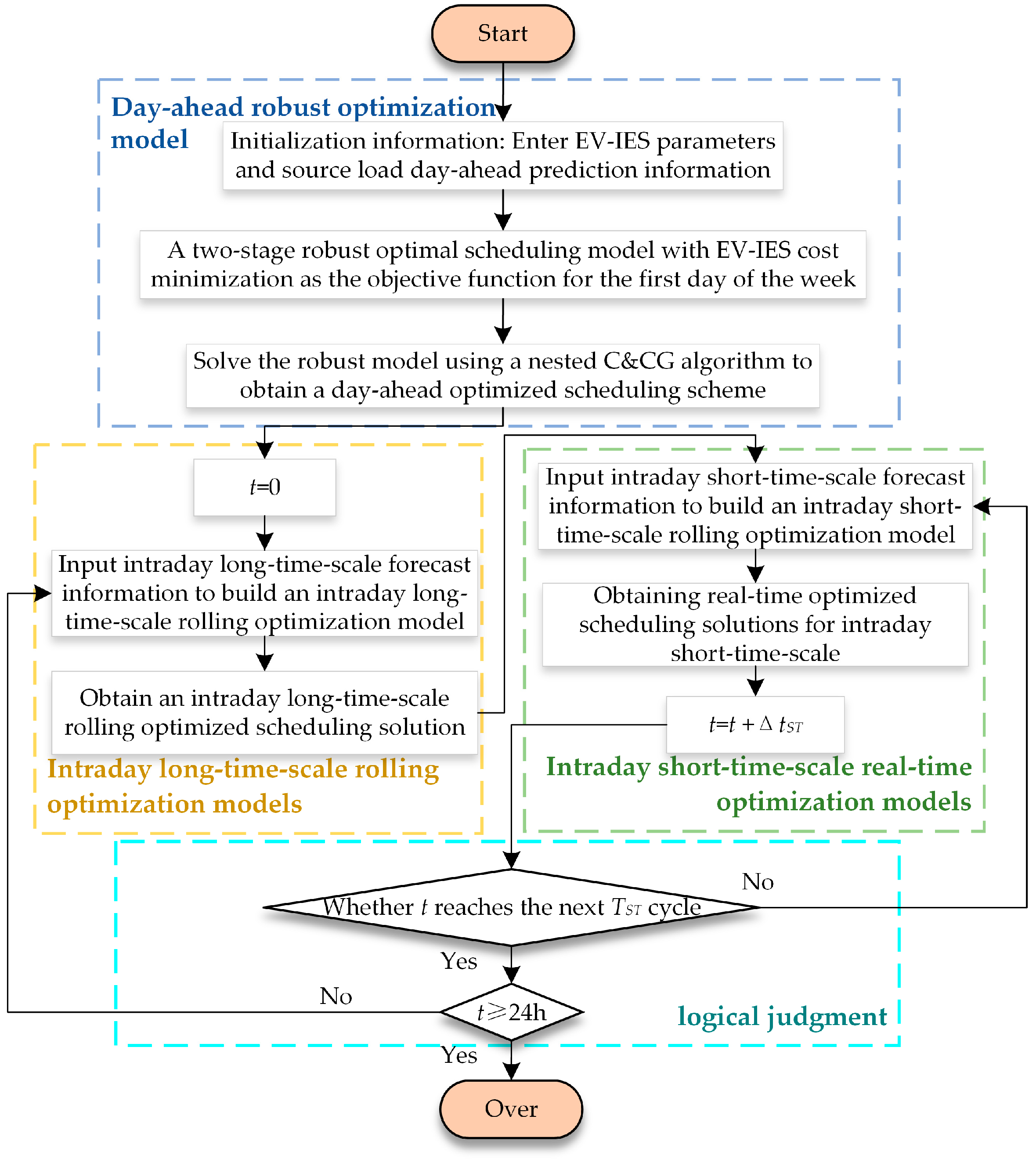
3.2. EV-IES Multi-Time-Scale Optimization Scheduling Strategy

To mitigate power fluctuations resulting from discrepancies between wind power and multiple load forecasts and actual intraday values, three optimization models are developed: a day-ahead optimization scheduling model, an intraday long-time-scale rolling optimization model, and an intraday short-time-scale, real-time optimization model. The day-ahead optimization scheduling model generates optimization strategies for each unit in EV-IES for one scheduling cycle. It utilizes day-ahead forecast information and considers source–load uncertainty as well as the N-1 contingency state of the system. It serves as a reference for the intraday optimization model. The intraday long time-scale rolling optimization model follows the day-ahead plan, combines the latest intraday forecast information, and redefines the operating state of each unit within the T_LT of the dispatch cycle. The intraday short-time-scale, real-time optimization model follows the day-ahead optimization and the intraday long-time-scale rolling optimization. According to the real-time forecast information, it updates the output status of each unit within the T_ST of the dispatch cycle.

3.2.1. Day-Ahead, Two-Stage Robust Optimization

The day-ahead scheduling of an EV-IES is a two-stage robust model, enhanced by improvements to the uncertainty set. In the first stage, it addresses the day-ahead minimization problem, while the second stage focuses on minimizing the objective function under the worst-case scenario of the uncertainty set.

$$\begin{array}{l}\underset{\mathit{x}}{\min }\left\{{\displaystyle \sum _{t=1}^T(}{C}_{uv})+\underset{\mathit{u}}{\max } \underset{\mathit{y},\mathit{z}}{\min }{\displaystyle \sum _{t=1}^T(C_{ps}+C_{mt})}\right\}\\ \mathit{x}=[x_t^{CHP},u_t^{CHP}]\\ \mathit{y}=\left[\begin{array}{l}{N}_{q,a,t},N_{q,c,t},N_{q,d,t},N_{all,c,t},N_{all,d,t},P_{all,c,t},P_{all,d,t},P_{buy},P_{sell},\\ P_t^{CHP},Q_t^{CHP},G_t^{CHP},Q_t^{GB},G_t^{GB},Q_t^{eh},P_t^{eh},R_t^{ec},P_t^{ec},R_t^{ac},Q_t^{ac},\\ P_{c,t}^e,P_{d,t}^e,E_t^e,P_{c,t}^h,P_{d,t}^h,E_t^h,P_{c,t}^c,P_{d,t}^c,E_t^c\end{array}\right]\\ \mathit{z}=\left[{\sigma }_{c,t}^b,{\sigma }_{c,t}^b,{\delta }_{i,c,t},{\delta }_{i,d,t},{\sigma }_{c,t}^e,{\sigma }_{d,t}^e,{\sigma }_{c,t}^h,{\sigma }_{d,t}^h,{\sigma }_{c,t}^c,{\sigma }_{d,t}^c\right]\\ \mathit{u}=[{\epsilon }_{\omega }^{b+},{\epsilon }_{\omega }^{b-},r]\end{array}$$

(30)

where x is the first-stage variable, including the operation variable and start variable of CHP, which is the decision variable of the day before. It is not affected by uncertainty. u is the second-stage uncertain variable, which can only change in the uncertain set and decide the worst case of the day. y and z include the continuous variable and discrete variable of multiple units. They carry out real-time adjustment after determining the worst case of the day to realize the minimization of the objective function.

3.2.2. Intraday Long-Time-Scale Rolling Optimization Model

The intraday long-time-scale rolling optimization obtains operation plans for multiple units based on the two-stage robust optimization from the previous day, including the start/stop status of CHP units, charging and discharging status of EVBSS, and charging/discharging status of the ES system.

$$\begin{array}{l}\underset{{\mathit{x}}_{\mathit{L}\mathit{T}},{\mathit{y}}_{\mathit{L}\mathit{T}},{\mathit{z}}_{\mathit{L}\mathit{T}}}{\min }{\displaystyle \sum _{t=1}^{T_{LT}}(C_{ps\cdot LT}+C_{mt\cdot LT})\Delta t_{LT}}\\ s.t.\left\{\begin{array}{l}{\mathit{x}}_{LT}=\mathit{x}\\ {\mathit{y}}_{LT}=\mathit{y}+\Delta {\mathit{y}}_{LT}\\ (1)-(26)\end{array}\right.\end{array}$$

(31)

where the subscript LT represents the intraday long-time-scale variable. Δy_LT is the deviation value of the intraday long-time-scale variable. The first constraint states that the start–stop variables of the CHP unit are determined by day-ahead robust optimization. The second constraint states that the intraday long-time-scale variable y_LT takes the day-ahead robust optimization result as the reference value. The rest of the constraints are the same as day-ahead robust optimization. Additionally, the WT, PV, electric load, heat load, and cold load are updated to the intraday long-time-scale rolling optimization predictions

3.2.3. Intraday Short-Time-Scale Real-Time Optimization Model

Intraday short-time-scale real-time optimization adjusts the scheduling plan of each unit again according to the short-term forecast information on the basis of day-ahead robust optimization and intraday long-time-scale rolling optimization. Intraday short time scale real-time optimization also does not consider short term forecast errors. The corresponding deterministic optimization model is as follows.

$$\begin{array}{l}\underset{{\mathit{x}}_{\mathit{S}\mathit{T}},{\mathit{y}}_{\mathit{S}\mathit{T}},{\mathit{z}}_{\mathit{S}\mathit{T}}}{\min }{\displaystyle \sum _{t=1}^{T_{ST}}(C_{ps\cdot ST}+C_{mt\cdot ST})\Delta t_{ST}}\\ s.t.\left\{\begin{array}{l}{\mathit{x}}_{ST}=\mathit{x}\\ {\mathit{y}}_{ST}={\mathit{y}}_{LT}+\Delta {\mathit{y}}_{ST}\\ (1)-(26)\end{array}\right.\end{array}$$

(32)

where the subscript ST represents the intraday short-time-scale variable. Δy_ST is the deviation value of the intraday short-time-scale variable. The first constraint states that the start–stop variables of the CHP unit are determined by day-ahead robust optimization. The second constraint states that the intraday short-time-scale variable y_ST takes the intraday long-time-scale optimization result as the reference value. The rest of the constraints are the same as day-ahead robust optimization. Additionally, the WT, PV, electric load, heat load, and cold load are updated to the intraday short-time-scale rolling optimization predictions.

3.3. Model Solving Method

For the convenience of subsequent description, the above two-stage robust model and constraints are simplified into the following matrix form.

$$\begin{array}{l}\underset{\mathit{x}}{\min }\left\{{\mathit{c}}^T\mathit{x}+\underset{\mathit{u}}{\max }\underset{\mathit{y},\mathit{z}}{\min }{\mathit{d}}^T\mathit{y}+{\mathit{g}}^T\mathit{z}\right\}\\ s.t.\hspace{1em}\mathit{A}\mathit{x}\le \mathit{b},\mathit{x}\in \left\{0,1\right\}\\ \mathit{C}\mathit{y}+\mathit{D}\mathit{z}+\mathit{E}\mathit{x}+\mathit{F}\mathit{u}\le \mathit{f},\mathit{z}\in \left\{0,1\right\}\end{array}$$

(33)

where c, d, and g are all cost coefficient vectors. A, C, D, E, and F are constraint coefficient matrices. b and f are constraint coefficient vectors. The second formula represents all constraints on x in the first stage. The third formula represents constraints on x, u, y, and z in the second stage.

Since the min–max–min robust model is non-convex and cannot be directly solved, the max–min problem in the second stage can be converted into the max–max form by using strong dual theory or KKT conditions. It can be merged into a single-layer max problem. Therefore, solving this robust model is equivalent to solving a two-stage mixed integer linear programming model. The C&CG algorithm is selected to decompose it into main problems and subproblems, gradually approaching the upper and lower bounds to obtain the optimal solution via interactive iteration [32]. However, the C&CG algorithm requires that the third-layer min problem only contains continuous variables, and z in Equation (33) belongs to discrete variables. It does not meet the strong dual theory and cannot directly solve the robust model. Therefore, this paper adopts the nested C&CG algorithm to transform and solve the min–max–min model, relaxing the restrictions on variables in the third-layer min problem. It decomposes the max–min problem into inner main problems and inner slave problems for solution.

3.3.1. The Main Problems

$$\begin{array}{l}\underset{\mathit{x},\eta }{\min } {\mathit{c}}^T\mathit{x}+\eta \\ s.t.\hspace{1em}\mathit{A}\mathit{x}\le \mathit{b}\\ \hspace{1em}\hspace{1em}\eta \ge {\mathit{d}}^T{\mathit{y}}_k+{\mathit{g}}^T{\mathit{z}}_k\\ \hspace{1em}\hspace{1em}\mathit{C}{\mathit{y}}_k+\mathit{D}{\mathit{z}}_k+\mathit{E}\mathit{x}+\mathit{F}{\mathit{u}}^{*}\le \mathit{f}\end{array}$$

(34)

where k is the number of iterations of the main problem. u* is the determined value after solving the slave problem. The main problem is a mixed integer linear programming problem, which can be directly solved using a commercial solver.

3.3.2. The Slave Problem

The slave problems can be expressed as follows:

$$\begin{array}{l}\eta =\underset{\mathit{u}}{\max } \underset{\mathit{y},\mathit{z}}{\min } {\mathit{d}}^T\mathit{y}+{\mathit{g}}^T\mathit{z}\\ s.t. \mathit{C}\mathit{y}+\mathit{D}\mathit{z}+\mathit{E}{\mathit{x}}^{*}+\mathit{F}\mathit{u}\le \mathit{f},\mathit{z}\in \left\{0,1\right\}\end{array}$$

(35)

where x* is the definite value after solving the main problem. However, due to the existence of discrete variable z, the dual transformation cannot be directly adopted. So, the C&CG algorithm is used to decompose Equation (35) into inner-main problem and inner-slave problem again.

The inner-slave problem

$$\begin{array}{l}\underset{\mathit{y},\mathit{z}}{\varphi =\min } {\mathit{d}}^T\mathit{y}+{\mathit{g}}^T\mathit{z}\\ s.t. \mathit{C}\mathit{y}+\mathit{D}\mathit{z}+\mathit{E}{\mathit{x}}^{*}+\mathit{F}{\mathit{u}}_n^{*}\le \mathit{f},\mathit{z}\in \left\{0,1\right\}\end{array}$$

(36)

where ${\mathit{u}}_n^{*}$ is the definite value after the nth iteration of the inner-main problem.

The inner-main problem

$$\begin{array}{l}\underset{u,\pi }{\max }\Phi \\ \Phi \le {\mathit{g}}^T{\mathit{z}}_n^{*}+{\mathit{\pi }}^T(\mathit{f}-\mathit{E}{x}^{*}-\mathit{F}\mathit{u}-\mathit{D}{\mathit{z}}_n^{*})\\ s.t. -{\mathit{\pi }}^{\mathrm{T}}\mathit{C}\le {\mathit{d}}^{\mathrm{T}}, \mathit{\pi }\ge 0,\end{array}$$

(37)

where π is the dual variable of variable y in Equation (35). $Z_n^{*}$ is the definite value after the nth iteration of inner-slave problem solving. Since the discrete variable z has been determined, only continuous variables exist in the second stage. The subproblem is transformed into a single-layer max problem according to the strong dual theory [33].

However, there is a nonlinear term π^Tu in Equation (37), which maintains the model as a non-deterministic polynomial (NP) hard problem [34]. Considering that the uncertain set has been discretized into multiple intervals, ${\epsilon }_{\omega ,t}^{b+}$ and ${\epsilon }_{\omega ,t}^{b-}$ in each interval are binary discrete variables. The following method can be used to convert it into a linear constraint.

$$\begin{array}{l}{\mathit{\pi }}^T\mathit{F}\mathit{u}={\displaystyle \sum _{\omega }{\displaystyle \sum _t{F}_{\omega ,t}[{\pi }_{\omega ,t}{P}_{\omega ,t}^{*}+{\displaystyle \sum _b({\pi }_{\omega ,t}{P}_{\omega ,t}^{b+}{\epsilon }_{\omega ,t}^{b+})}}}-{\displaystyle \sum _b({\pi }_{\omega ,t}{P}_{\omega ,t}^{b-}{\epsilon }_{\omega ,t}^{b-})}]\\ \hspace{1em}\hspace{1em} ={\displaystyle \sum _{\omega }{\displaystyle \sum _t{F}_{\omega ,t}[{\pi }_{\omega ,t}{P}_{\omega ,t}^{*}+{\displaystyle \sum _b{P}_{\omega ,t}^{b+}{\mu }_{\omega ,t}^{+}}}}-{\displaystyle \sum _b{P}_{\omega ,t}^{b-}{\mu }_{\omega ,t}^{-}}]\hspace{1em}\hspace{1em}\forall u\in \omega ,{\mu }_{\omega ,t}^{+},{\mu }_{\omega ,t}^{-}\in \left\{0,1\right\}\end{array}$$

(38)

$$\left\{\begin{array}{l}-\mathrm{M}{\epsilon }_{\omega ,t}^{b+}\le {\mu }_{\omega ,t}^{+}\le \mathrm{M}{\epsilon }_{\omega ,t}^{b+}\\ {\pi }_{\omega ,t}-\mathrm{M}(1-{\epsilon }_{\omega ,t}^{b+})\le {\mu }_{\omega ,t}^{+}\le {\pi }_{\omega ,t}+\mathrm{M}(1-{\epsilon }_{\omega ,t}^{b+})\\ -\mathrm{M}{\epsilon }_{\omega ,t}^{b-}\le {\mu }_{\omega ,t}^{-}\le \mathrm{M}{\epsilon }_{\omega ,t}^{b-}\\ -{\pi }_{\omega ,t}-\mathrm{M}(1-{\epsilon }_{\omega ,t}^{b-})\le {\mu }_{\omega ,t}^{-}\le -{\pi }_{\omega ,t}+\mathrm{M}(1-{\epsilon }_{\omega ,t}^{b-})\end{array}\right.$$

(39)

where ${\mu }_{\omega ,t}^{+}$ and ${\mu }_{\omega ,t}^{-}$ are auxiliary variables. In Equation (38), there is the case where the continuous variable $P_{\omega ,t}^{b+}$ is multiplied by the bivariate variable ${\epsilon }_{\omega ,t}^{b+}$. It is a nonlinear constraint. In order to linearize it, the auxiliary variables ${\mu }_{\omega ,t}^{+}$ and ${\mu }_{\omega ,t}^{-}$ are introduced and transformed by Equation (39). In Equation (39), the range of ${\mu }_{\omega ,t}^{+}$ and ${\mu }_{\omega ,t}^{-}$ is limited by the big M method. If ${\epsilon }_{\omega ,t}^{b+}$ = 0, then ${\mu }_{\omega ,t}^{+}$ is also equal to 0. If ${\epsilon }_{\omega ,t}^{b+}$ = 1, then ${\mu }_{\omega ,t}^{+}$ is equal to п_ω,t. ${\mu }_{\omega ,t}^{-}$ is the same.

For N-1 contingency variables r_GB, r_ac, r_eh, and r_ec in the uncertain set, the big M method is also adopted for linear transformation. Take Equation (14) containing r_GB as a case:

$${\pi }^T{F}_{gb}{r}_{gb}={\displaystyle \sum _{\omega }{\displaystyle \sum _t{F}_{gb,t}({\pi }_{gb,t}{r}_{gb})}}={\displaystyle \sum _{\omega }{\displaystyle \sum _t{F}_{gb,t}{R}_{gb,t}}},$$

(40)

$$\left\{\begin{array}{l}-\mathrm{M}{r}_{gb}\le R_{gb,t}\le \mathrm{M}{r}_{gb}\\ {\pi }_{gb,t}-\mathrm{M}(1-r_{gb})\le R_{gb,t}\\ R_{gb,t}\le {\pi }_{gb,t}+\mathrm{M}(1-r_{gb})\end{array}\right.$$

(41)

where R_gb is an auxiliary variable. The remaining N-1 contingency variables can be converted in accordance with the same method.

3.3.3. Solving Process of Nested C&CG Algorithm

The solving process of the nested C&CG algorithm is shown in Algorithm 1. Its specific steps are as follows:

• Initialization: Set the number of iterations as k = 1. Give the convergence threshold ε. Give a set of feasible solutions of the main problem x₀, and bring them into the slave problem Equation (35) to obtain u_k, y_k, and z_k. Set the upper bound UB = +∞ and the lower bound LB = −∞.
• Substitute u_k into the main problem Equation (34) to solve for ${\mathit{x}}_{*k}$, and update the lower bound LB = min {LB, c^Tx_k + η_k}.
• Substitute x_k into the slave problem Equation (35) to solve u_k+1, y_k+1, and z_k+1. The steps are as follows:

  (1)

  Initialization: Set the number of subproblem iterations n = 1. Give a set of u₀ as the feasible solution of the inner-slave problem, and solve the inner-slave problem with u₀ and x_k to obtain y_n and z_n. Set the upper bound of the subproblem UB_in = +∞ and the lower bound of the subproblem LB_in = −∞.

  (2)

  Substitute x_k and z_n into the inner-main problem Equation (37) to solve for u_n and Φ_n, and update LB_in = Φ_n.

  (3)

  Substitute x_k and u_n into the inner-slave problem Equation (36) to solve for z_n+1 and ϕ_n, and update UB_in = ϕ_n.

  (4)

  If UB_in − LB_in < ε, then stop the iteration, output u_n, z_n+1, and Φ_n, and update LB =c^Tx_k + Φ_n. Otherwise, set n = n + 1, and return to (2) to continue the solution.

• If UB − LB < ε, stop the iteration and output the best result. Otherwise, set k = k + 1 and return to 2 to continue solving.

Algorithm 1. Solving process of nested C&CG algorithm

1: Initial LB = −∞, UB = ∞, k = 1, and ε, and solve the slave problem with x0 to obtain uk, yk, and zk

Repeat

2: Solve the main problem with uk to obtain (xk and ηk),       and update LB = min {LB, cTxk + ηk}.

3: Solve the slave problem with xk to obtain (uk+1, yk+1, and zk+1).

Repeat

(1) Initial LBin = −∞, UBin = +∞, n = 1, and ε, and solve the inner-slave problem       with (xk, u0) to obtain (yn, zn).

(2) Solve the inner-main problem with (xn and zn) to obtain (un and Φn),       and update LBin = Φn.

(3) Solve the inner-salve problem with (xn and un) to obtain (zn+1 and ϕn),       and update UBin = ϕn.

(4) n = n + 1.

Until UBin − LBin < ε, output (un+1, yn+1, zn+1, and Φn), and update UB = cTxk + Φn.

4: k = k + 1.

Until UB − LB < ε, output the best result.

3.3.4. Multi-Time-Scale Model Solution

The EV-IES multi-time-scale optimal scheduling strategy solution flow is shown in Figure 4.

First, we entered the initialization information: the parameters of all units in the EV-IES and the predicted values and deviation limits of all uncertain variables. Then, the nested C&CG algorithm was used to solve the two-stage robust model Equation (30). The solution results x, y, and z are passed to the day-ahead long-time-scale rolling optimization model as day-ahead optimization schemes.

Second, enter intraday long-time-scale forecast information, including the actual values of all uncertain variables. According to the results of day-ahead robust optimization, the deterministic scheduling model Equation (31) is solved. The power of each unit is redistributed to obtain intraday long-time-scale scheduling results.

Finally, enter the forecast information for a short-time-scale within the day. According to the day-ahead robust optimization scheme and long-time-scale rolling optimization results, short-time-scale model Equation (32) is solved. A short-time-scale real-time optimization scheme is obtained.

4. Case Study

The grid purchase price adopts time-of-use electricity price. Peak periods: 10:00–15:00 and 18:00–21:00, 1.5 CNY/kWh. Normal periods: 7:00–10:00, 15:00–18:00, and 21:00–23:00, 1.35 CNY/kWh. Valley period: 23:00–7:00, 1.1 CNY/kWh. The other parameters are shown in

Table 2. Parameter of IES.

	Parameter	Value	Parameter	Value	Parameter	Value	Parameter	Value
EVBSS	K	7	$P_c^{EV}$	5 kW	$P_c^{EV}$	4.5 kW	T	24 h
	Δt	1 h	Nmax	300
	[S1,t S2,t]	[0.15 0.25]	[S2,t S3,t]	[0.25 0.35]	N1,a,0	260	N2,a,0	25
	[S3,t S4,t]	[0.35 0.45]	[S4,t S5,t]	[0.45 0.55]	N3,a,0	25	N4,a,0	30
	[S5,t S6,t]	[0.55 0.65]	[S6,t S7,t]	[0.65 0.75]	N5,a,0	25	N6,a,0	35
	[S7,t S8,t]	[0.75 0.85]			N7,a,0	300
CHP	${\eta }_{dis}^{CHP}$	0.45	$P_{\min }^{CHP}$	400 kW	$P_{\max }^{CHP}$	1000 kW	ηCHP	0.3
	$m_u^{CHP}$	20 CNY	mCHP	0.03 CNY/kWh	Lng	9.7 kWh/m3
GB	ηGB	0.93	$Q_{\max }^{GB}$	1000 kW	mgas	2.8 CNY/m3	mGB	0.005
EHCE	Ceh	2.8	$P_{\max }^{eh}$	2000 kW
ECCE	Cec	2.8	$P_{\max }^{ec}$	800 kW
AC	Cac	1.2	$R_{\max }^{ac}$	1000 kW
Energy storage system	$E_0^e$	1500 kWh	${\eta }_{dis}^e$	0.92	${\eta }_{ch}^e$	0.93	${\lambda }_{\min }^e$	0.2
	${\lambda }_{\max }^e$	0.9	$E_n^e$	2000 kWh	$P_{c,\max }^e$	1000 kW	$P_{d,\max }^e$	1000 kW
	$E_0^h$	1200 kWh	${\eta }_{dis}^h$	0.93	${\eta }_{ch}^h$	0.93	${\lambda }_{\min }^h$	0.1
	${\lambda }_{\max }^h$	0.9	$E_n^h$	2000 kWh	$P_{c,\max }^h$	500 kW	$P_{d,\max }^h$	500 kW
	$E_0^c$	1200 kWh	${\eta }_{dis}^c$	0.92	${\eta }_{ch}^c$	0.92	${\lambda }_{\min }^c$	0.1
	${\lambda }_{\max }^c$	0.9	$E_n^c$	2000 kWh	$P_{c,\max }^c$	500 kW	$P_{d,\max }^c$	500 kW
	τh, τc	0.99	mes	0.005 CNY/kWh	mhs, mhc	0.001 CNY/kWh
Utility grid	Pb,max	2000 kW	Ps,max	2000 kW	msell	0.4 CNY/kWh

. Figure 5 shows the predicted values and error intervals of wind power, PV power, electric load, heat load, and cold load. The number of electric vehicle battery exchanges in each period. The prediction deviations of wind power and PV power generation are set as three intervals. The deviations are ±10%, ±5%, and ±2% of the predicted values, respectively. The errors of electric, heat, and cold loads are set as one interval. The deviations are all ±5% of the predicted values. The deviation budgets of each interval in the WT {${\mathrm{\Pi }}_{\mathrm{W}\mathrm{T}}^1$, ${\mathrm{\Pi }}_{\mathrm{W}\mathrm{T}}^2$, ${\mathrm{\Pi }}_{\mathrm{W}\mathrm{T}}^3$} are set as {1, 2, 7}, respectively. The deviation budgets of each interval in PV power generation {${\mathrm{\Pi }}_{\mathrm{P}\mathrm{V}}^1$, ${\mathrm{\Pi }}_{\mathrm{P}\mathrm{V}}^2$, ${\mathrm{\Pi }}_{\mathrm{P}\mathrm{V}}^3$} are set as {1, 2, 5}, respectively. The budget deviations of basic electric load, heat load, and cold load {${\mathrm{\Pi }}_{\mathrm{P}\mathrm{L}}^1$, ${\mathrm{\Pi }}_{\mathrm{Q}\mathrm{L}}^1$, ${\mathrm{\Pi }}_{\mathrm{R}\mathrm{L}}^1$} are set as {8, 8, 8}, respectively. In order to verify the effectiveness of the proposed robust model, the optimized scheduling model is developed using MATLAB and solved using CPLEX via YALMIP.

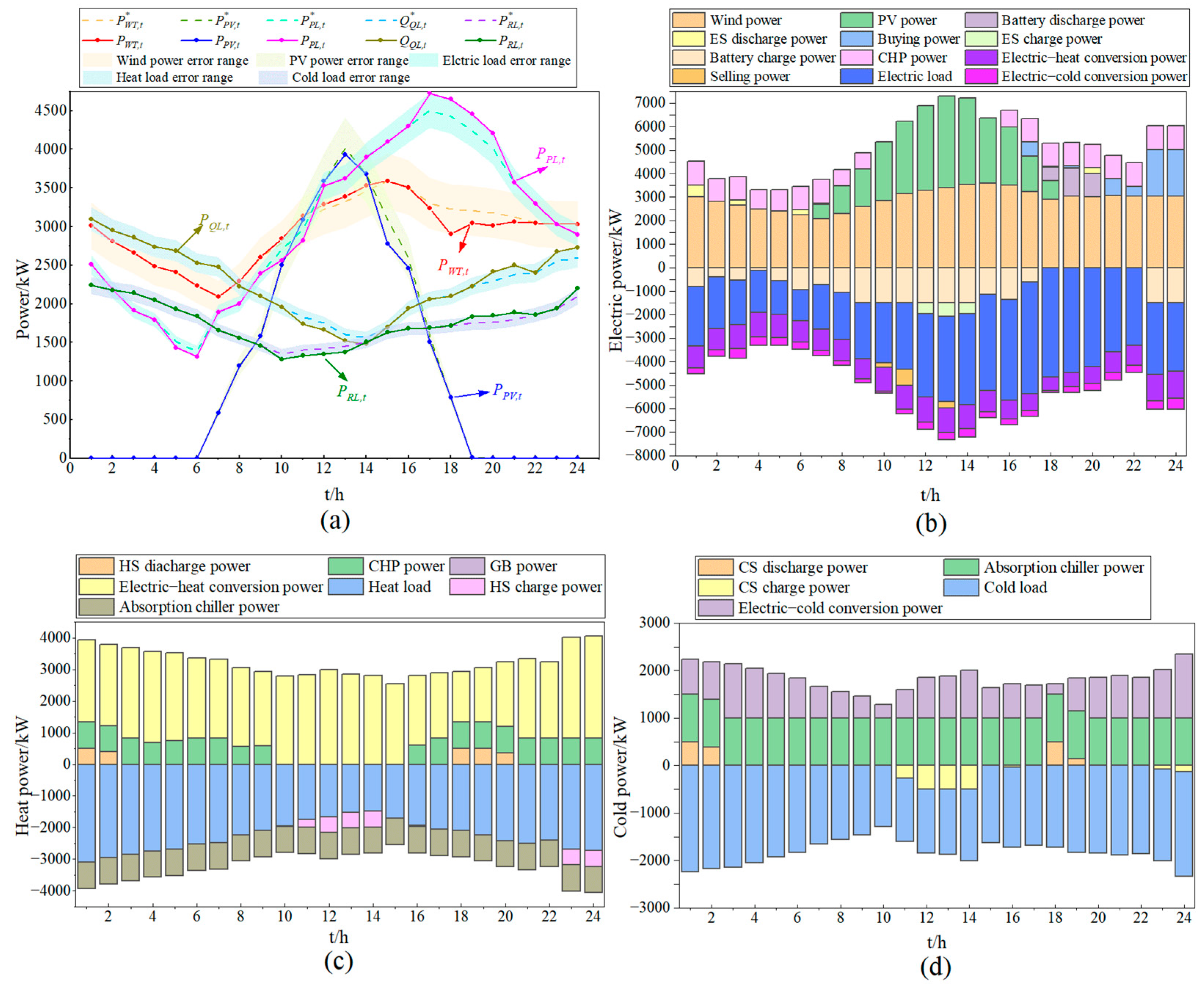
4.1. IES Optimal Scheduling Scheme without N-1 Contingency States

Since the system is less likely to experience N-1 contingency, the proposed method can also be applied during normal system operation, requiring only the setting of the value of П_r in Equation (29) to 4. The optimal scheduling scheme of the EV-IES is shown in Figure 6. The total cost of IES is CNY 22,539.

From Figure 6a, it can be observed that, when considering only the uncertainty of the power source and load, the WT experiences lower deviation during 18:00–21:00 and 24:00, while upper deviation primarily occurs during 11:00–14:00. Lower deviation for PV power generation happens at 10:00, 13:00, 15:00–16:00, and other times. Lower deviation for electric load occurs at 3:00–6:00 and 11:00, with upper deviation occurring at 18:00–21:00. Combining with Figure 6b, it can be seen that, during the periods of 1:00–9:00 and 17:00–24:00, CHP needs to assist with higher power generation to meet the system’s power demand due to minimal or no PV power generation. Particularly during 18:00–21:00, the actual electric load is high, while PV power generation is low. The system faces a severe shortage of power. At this time, the battery cluster and ES system at the EV charging station release their stored energy to maintain balance. It can be seen that battery clusters can not only meet the user’s swapping needs, but also work with the ES system to assist in peak shifting. In the period of 23:00–24:00, the IES has to purchase excess power from the grid to fulfill the swapping needs of EV users. It also need to conserve energy within the battery cluster over a dispatch cycle. Despite the low electricity price during this time, the system cost still increases significantly. From 10:00 to 16:00, although the actual values of wind and PV power are reduced to varying degrees, the IES still has excess power for charging other devices, owing to substantial PV power generation. Thus, CHP ceases operation. The battery cluster and ES system charge at high power. Even in the periods of 11:00 and 14:00, the system also sells excess power to the power grid to obtain additional income under the premise of full load of the ES system.

The lower deviations of both heat and cold loads mainly occur during 11:00–14:00, while the upper deviations are mostly concentrated during 18:00–24:00. As can be seen from Figure 6c,d, the EHCE and ECCE need to operate continuously to maintain the balance of heat and cold power. During the noon period, the actual value of the heat load is small. The energy of the IES is abundant. So, the EHCE can provide all the heat power and provide excess heat power for the ES equipment. However, the heat load reaches its maximum deviation during 19:00–24:00, especially during 17:00–24:00. The CHP unit and gas-fired boiler need to operate simultaneously to meet the rapidly increasing heat load demand.

Since there is no direct cold equipment in the IES, the cold power must be provided by absorption refrigeration or electricity-to-cold conversion equipment. Therefore, the AC machine operates at full power in all periods. Since electric power is abundant during the noon period, the electricity-to-cold conversion equipment can also provide a large amount of cold power. The ES system continues to store cold energy. However, almost all the cold power is used to meet the load demand due to the high cold load during the rest of the time.

Figure 6e and Figure 6f, respectively, display the number and power of charged and discharged batteries, as well as the number of batteries in each interval. During the period of 9:00–14:00, the number of charged batteries reaches the maximum value of 300 and the charging power is also maintained at the maximum value due to a large amount of PV power generation. In the period of 18:00–22:00, the batteries begin to discharge electricity to maintain the stability of THE system power due to the almost-zero PV power generation and the extreme lack of electric energy. At the same time, when the batteries are charged, they follow the order of N_6,c,t, N_5,c,t, N_4,c,t, N_3,c,t, N_2,c,t, and N_1,c,t, so as to ensure that the number of charged batteries is always greater than the number of users’ demands. When the batteries are discharged, they follow the order of N_2,c,t, N_3,c,t, N_4,c,t, N_5,c,t, N_6,c,t, and N_7,c,t.

4.2. IES Optimal Scheduling Scheme Considering N-1 Contingency States

If N-1 contingency occurs in the system, the contingency budget in Equation (29) is set as three. The results are shown in Figure 7.

As shown in Figure 7a, the lower deviation of wind power occurs between 17:00–21:00, while the upper deviation mainly occurs between 10:00–14:00. The lower deviation of PV power occurs at 12:00 and 15:00–17:00. The lower deviation of electric load occurs at 5:00–6:00 and 10:00–11:00. The upper deviation occurs at 17:00–20:00. It can be clearly seen in Figure 7c that the power of the GB remains at 0. It indicates that the GB in the worst-case scenario. This also indicates that the electric–heat conversion equipment must operate at maximum power. This is supplemented by CHP heating and heat release from the ES system to maintain heat power balance during the period from 17:00 to 24:00 when the heat load is high and upper deviations occur repeatedly. At the same time, the system is at various critical points of energy shortage during this period. Therefore, the IES must achieve energy time shifting through battery clusters and ES systems. It is necessary to purchase part of the electric energy from the grid when compensating for energy shortages. During the period from 10:00 to 15:00, the system can achieve heat power balance by shutting down the CHP equipment and relying solely on the electric–heat conversion equipment due to the small actual value of the heat load. It can also heat the HS system. During the period from 1:00 to 9:00, CHP must be used to assist in heat generation to ensure the stable operation of the system as the heat load exceeds the maximum value of the electric–heat conversion equipment. Overall, the failure of the gas-fired boilers results in the system having to purchase more power from the grid to achieve power balance during peak load periods. So, the IES cost rises rapidly to CNY 23,755, which is about 5.4% higher than the operating cost without considering the N-1 contingency status.

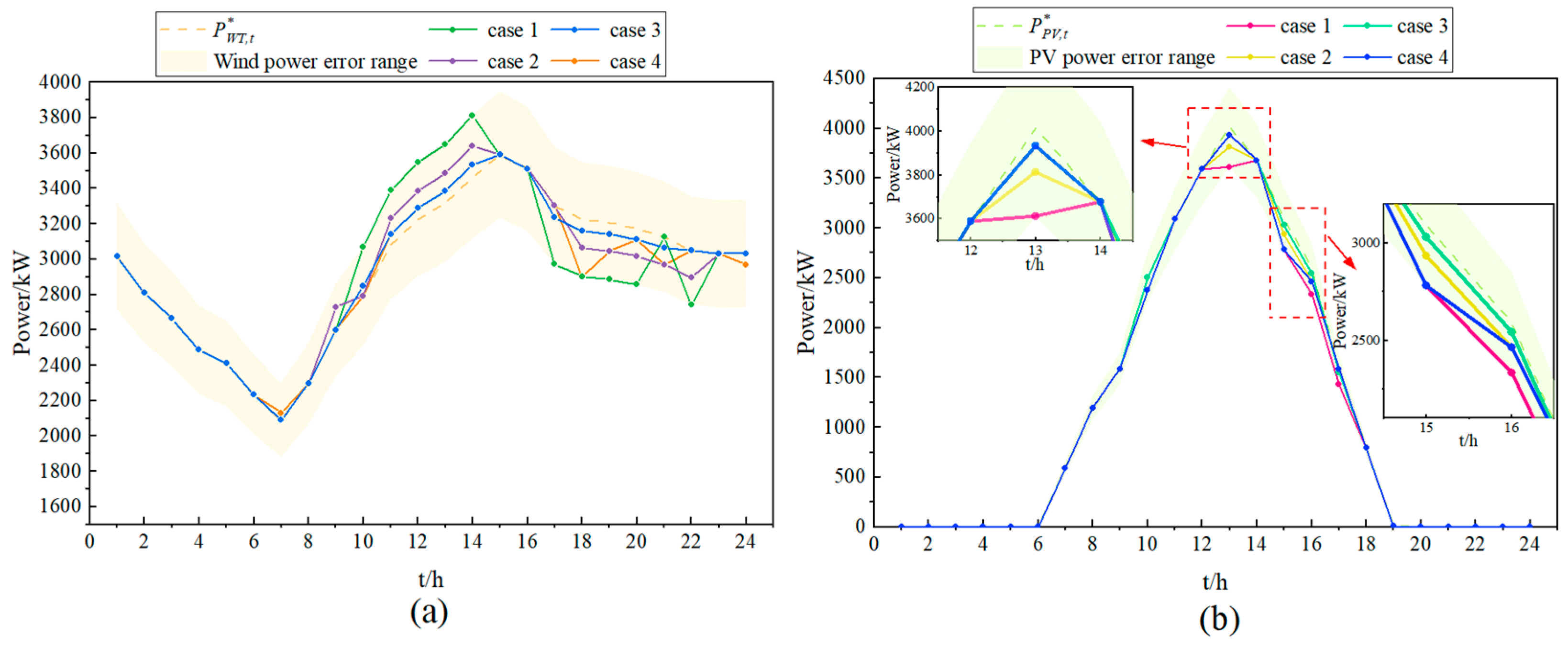
4.3. Multi-Interval Uncertainty Set Analysis

To verify the effectiveness of the proposed multi-interval uncertainty set, the following calculation cases are set up for comparative analysis. The results of WT and PV power generation are shown in Figure 8. The IES costs are presented in

Table 3. IES costs under different uncertain sets.

	Case 1	Case 2	Case 3	Case 4
Cost/CNY	28,133	24,558	23,312	22,539

.

Case 1: The original uncertainty set of Equation (27) is adopted.

Case 2: Use the first constraint, second constraint, and third constraint of Equation (28) as the uncertainty set.

Case 3: Equations (27) and the fourth constraint of Equation (28) are adopted as the uncertainty set.

Case 4: Equation (28) is adopted as the uncertainty set (this paper).

As shown in Figure 8a, the actual values of wind power in Case 1 and Case 2 both decline from 15:00 to 24:00. The difference lies in the fact that it reached the extreme deviation point every time in Case 1. In Case 2, it only occurred once, with the rest falling within a smaller deviation interval. To achieve symmetry in deviation occurrences, in Case 3, wind power increased from 10:00 to 14:00. It decreased from 17:00 to 20:00 and 22:00. In Case 4, wind power increased at 7:00 and 11:00 to 14:00. It decreased from 18:00 to 21:00 and at 24:00.

As shown in Figure 8b, the actual values of PV power generation in Case 1 and Case 2 both exhibit downward deviation from 10:00 to 17:00. The difference lies in the fact that it reaches the extreme deviation point every time in Case 1. In Case 2, the most serious deviation occurs only at 15:00. Case 3 has a downward deviation from 13:00 to 15:00. Case 4 has a downward deviation from 10:00 to 13:00 and 15:00 to 16:00.

Overall, in Case 1, all deviations of uncertainties reach the extreme deviation point. All deviations are in the same direction, which makes the worst-case scenario too radical and the scheduling scheme overly conservative. As shown in Table 3, the IES cost is CNY 28,133 at this time, which is approximately 24.8% higher than that in Case 4. In Case 2, although the uncertainty set is discretized finitely, all deviations still occur in the same direction in the worst-case scenario. Despite the significant cost reduction, it is still unreasonable. In Case 3, introducing deviation symmetry makes the upper and lower deviations equally and effectively reduce the IES cost. However, both the upper and lower deviations reach the extreme points of the deviation interval. The deviations are significant. In Case 4, the system cost can be freely selected within multiple deviation intervals. The number of small deviation intervals obtained using wind power or the actual value of PV power limited by the deviation budget is far greater than that of large deviation intervals. It reduces the system cost effectively. Compared with Case 2 and Case 3, the cost of Case 4 is reduced by approximately 8.96% and 3.43%, respectively. It indicates that the improved uncertainty set proposed in this paper can effectively reduce the conservatism of the uncertainty set and balance the economic benefits of IES.

A sensitivity analysis of the multi-interval uncertainty ensemble is conducted to limit the number of fluctuations in the new energy output by varying the parameter ${\mathrm{\Pi }}_{bW}$. The results are displayed in

Table 4. Multi-interval uncertainty ensemble sensitivity analysis.

WT	Case	${\mathrm{\Pi }}_{WT}^1$	${\mathrm{\Pi }}_{WT}^2$	${\mathrm{\Pi }}_{WT}^3$	Cost/CNY	PV	Case	${\mathrm{\Pi }}_{PV}^1$	${\mathrm{\Pi }}_{PV}^2$	${\mathrm{\Pi }}_{PV}^3$	Cost/CNY
	1	10	0	0	23,718		1	8	0	0	21,906
	2	7	1	2	23,155		2	6	1	1	21,668
	3	4	2	4	22,409		3	4	1	3	21,345
	4	1	3	6	21,617		4	2	2	4	20,934
	5	0	2	8	21,190		5	0	0	8	20,526
	6	0	0	10	20,957		6	0	4	4	20,749
	7	0	6	4	21,643		7	0	6	2	20,888
	8	0	10	0	21,993		8	0	8	0	20,984

.

From Case 1 to Case 4 in Table 4, it can be observed that the IES cost gradually reduces as parameters ${\mathrm{\Pi }}_{WT}^1$ and ${\mathrm{\Pi }}_{PV}^1$ decrease. The lowest system cost occurs when they reach zero. The reason is that they limit the actual values of wind and PV power generation within the maximum deviation range (±10%). Reducing ${\mathrm{\Pi }}_{WT}^1$ and ${\mathrm{\Pi }}_{PV}^1$ can gradually increase the wind and PV power obtained by the system, making the system operation more economical. For parameters ${\mathrm{\Pi }}_{WT}^2$ and ${\mathrm{\Pi }}_{PV}^2$, it is evident that the IES cost will increase with their growth (Case 5, Case 7, and Case 8) when ${\mathrm{\Pi }}_{WT}^1$ and ${\mathrm{\Pi }}_{PV}^1$ remain unchanged. The reason is that the growth of ${\mathrm{\Pi }}_{WT}^2$ and ${\mathrm{\Pi }}_{PV}^2$ inevitably leads to a decrease in ${\mathrm{\Pi }}_{WT}^2$ and ${\mathrm{\Pi }}_{PV}^3$. If the number of occurrences where the actual value falls within the small deviation interval (±2%) decreases, it will inevitably fall more times within the medium deviation interval (±5%). This results in a decrease in the actual power output of new energy sources. The system has to obtain power through other units to increase costs. Overall, when the actual value falls near the boundary of a larger deviation interval, the IES cost rapidly increases. The scheduling results tend to be conservative. When the actual value falls near the boundary of a smaller deviation interval, the IES cost gradually decreases. However, although this approach achieves better economic performance, it reduces the robustness of the system. When the system encounters a worse actual situation within the day, it may incur greater costs. Therefore, it is necessary to allocate uncertain budget parameters reasonably to balance the robustness and economic efficiency of the system.

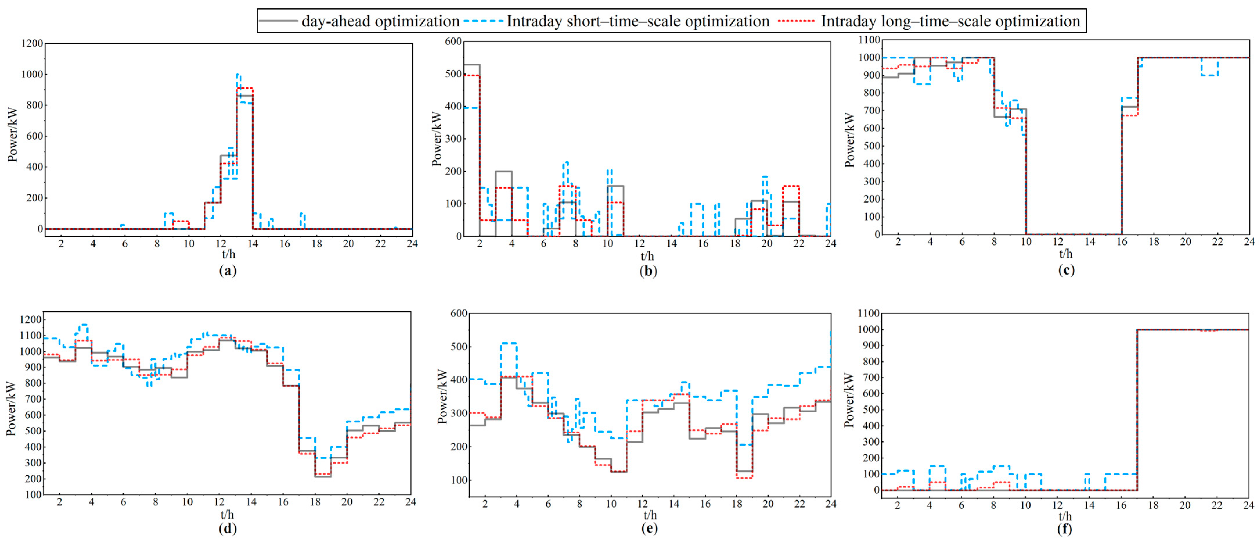
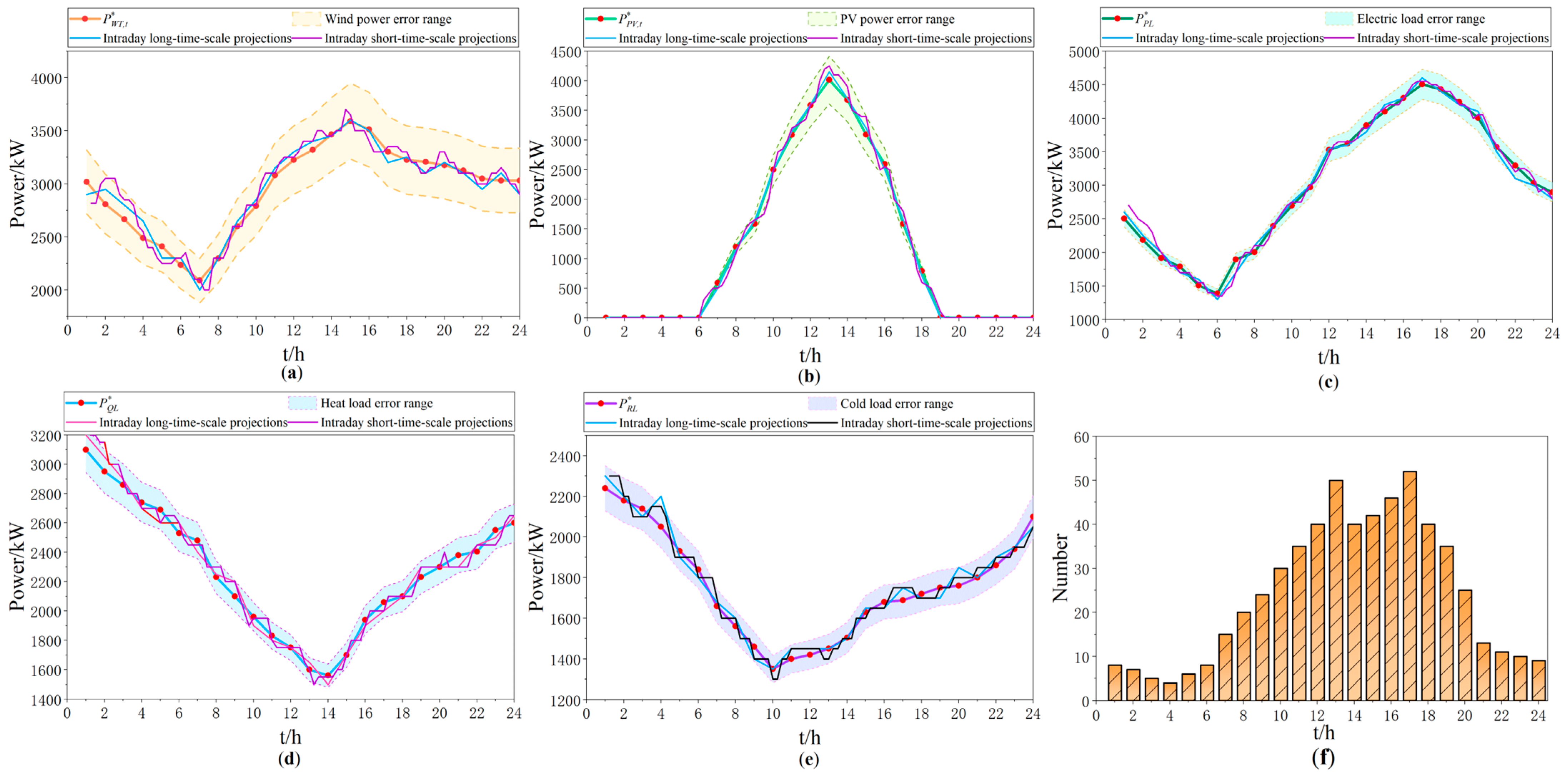
4.4. Analysis of Intraday Multi-Time-Scale Optimal Scheduling Results

The scheduling results obtained from the robust optimization in Section 4.1, which does not consider the system N-1 fault status, are used as the day-ahead plan. The partial results of intraday long-term rolling optimization and intraday short-term real-time optimization are shown in Figure 9.

Combining Figure 5a,b, it can be seen that there are significant deviations between the intraday forecast values and the day-ahead forecast values for wind power generation during 1:00–4:00, 9:00–14:00, and 16:00–20:00. The intraday forecast values exceed the day-ahead forecast values during 12:00–15:00 for PV power generation. The intraday forecast values and day-ahead forecast values of electric load exhibit significant deviations during 1:00–3:00, 6:00–8:00, and 21:00–24:00. The power deviation is primarily adjusted through the CHP and ES system. Taking 21:00–22:00 as an example for analysis, the intraday forecast value of the electric load is lower. Although there is some deviation in wind power generation, it Is relatively small. There is no output from PV power generation. At this time, the overall load of the system is low. There is sufficient electricity. Therefore, in Figure 9a–c, the output of the CHP unit decreases while the discharge of ES decreases simultaneously. Overall, the system charges the ES unit at a higher rate due to the high output of PV power generation during 12:00–14:00. In other periods, the system lacks electrical energy due to the lower output of PV power generation. The ES unit frequently discharges. It is supplemented by the CHP unit to generate electricity. The overall trend is similar to that of day-ahead robust optimization. For the heat load, there are significant deviations between the day-ahead forecast values and the intraday forecast values during 1:00–3:00, 8:00–11:00, and 19:00–22:00. For the cold load, the number of occurrences of upper deviations in the intraday forecast values compared to the day-ahead forecast values is much higher than that of lower deviations. This will lead to an overall overestimation of the cold load during intraday scheduling. Therefore, the power of the electric–cold conversion equipment is numerically overestimated in the results of long-time-scale and short-time-scale optimization in Figure 9e.

4.5. Analysis of Battery Charge and Discharge Prioritization Algorithm

In this paper, large-scale battery clusters are categorized based on their current charge level, followed by the introduction of a charge and discharge priority function. The effectiveness of the charge and discharge priority function is then analyzed through numerical examples. The cost of each numerical example is shown in

Table 5. IES cost analysis.

	Case 1	Case 2	Case 3
Electricity purchasing cost/CNY	3030	3030	4427
Electricity selling income/CNY	397.6	397.6	0
Total cost/CNY	22,539	22,539	24,959

. The number of batteries for N_L,a,t and N_1,a,t are illustrated in Figure 10.

Case 1: Adopting the charge and discharge priority function (this paper).

Case 2: Without the charge or discharge priority function.

Case 3: Batteries are only allowed to charge.

According to Table 5, it can be seen that the total costs of Case 1 and 2 are the same, but Case 3 cannot discharge during peak system loads due to the batteries only being able to charge. It has to purchase additional electricity from the grid, resulting in a rapid increase in purchased electricity costs. Compared to Case 1, the purchased electricity costs have increased by 46.1%. The total costs have increased by 10.7%. Therefore, the introduction of battery discharge functionality makes battery scheduling more flexible. It plays a role in peak shaving and valley filling effectively for reducing costs. Figure 10a shows the numbers of batteries in the N_L,a,t interval. It can be seen that all three examples can meet the battery replacement needs of EV users at any time, but the number of batteries varies significantly in each period. In Case 1, the charging and discharging priority function is to prioritize charging batteries with higher SOC, thus keeping N_L,a,t at a higher level throughout. Simultaneously, it ensures that a greater number of batteries have lower charging levels compared to Case 2. In Case 3, since batteries can only be charged, N_L,a,t remains consistently above 300. In Case 2, due to the system’s ability to allocate batteries freely, N_L,a,t is lower for most time periods compared to the other two cases. Additionally, the quantity of batteries is at a lower level during the 19:00–24:00 period. Given that Case 1 has more batteries and ES capacity compared to Case 3, it holds a comparative advantage in emergency situations. Overall, the introduction of the charge and discharge priority function makes battery scheduling more flexible. It enables better control of the system’s total costs. Additionally, there are more batteries with higher charge levels and lower charge levels, which can better respond to emergencies.

4.6. Analysis of Nested C&CG Algorithm

Since the third layer variable in Equation (33) contains binary discrete variables, the nested C&CG algorithm is adopted for solving. This section compares and analyzes the calculation cases of different solving methods. The results are shown in

Table 6. IES cost under different algorithms.

	Case 1	Case 2	Case 3	Case 4	Case 5
Cost/CNY	20,227	28,430	24,377	27,940	23,755

. The calculation cases are set as follows:

Case 1: Deterministic optimal scheduling model.

Case 2: The original uncertainty set of Equation (27) is adopted and the traditional C&CG algorithm is adopted for solving.

Case 3: The improved uncertainty set is adopted and the traditional C&CG algorithm is adopted for solving.

Case 4: The original uncertainty set of Equation (27) is adopted and the nested C&CG algorithm is adopted for solving.

Case 5: The improved uncertainty set is adopted and the nested C&CG algorithm is adopted for solving.

When deterministic optimal scheduling is used, the IES operating cost is only CNY 20,227. At this time, the predicted and actual values of uncertain quantities are equal. Although the system operating cost is the lowest, the likelihood of this occurring is relatively small. Once the uncertain variables fluctuate, the IES will call for more resources to keep the system stable. At this time, the operating cost will be substantially increased.

Both Case 2 and Case 4 adopt the original uncertainty set. This will lead to the extreme point of deviation for uncertain parameters in many instances. It often tends towards the same direction. This is quite different from the actual situation. Compared with Case 5, the total cost of Case 2 and Case 4 is increased by about 19.68% and 17.62%, respectively. The results are too conservative. Both Case 3 and Case 5 adopt the improved uncertainty set, but Case 3 needs to determine the variables of multiple devices before the day. Although the calculation of intraday scenarios is reduced, it is impossible to readjust the variables of each unit when the actual value differs significantly from the predicted value. A small number of transactions with the power grid is needed to balance the load. While Case 5 adopts the nested C&CG algorithm, the system will readjust the scheduling plan to meet the operational requirements of the system when any scenario in the uncertainty set occurs. Compared with Case 3, the operating cost of the IES is reduced by about 2.62%, proving the effectiveness of the algorithm.

5. Conclusions

In this paper, an IES optimal scheduling strategy based on an improved uncertainty set is proposed for IESs with EVBSSs. The following conclusions can be drawn:

(1)

Integration of EVBSSs in IESs not only meets the battery swapping needs of EV users but also utilizes large-scale battery clusters to co-schedule with ES for better energy transfer.

(2)

Limited discretization of the deviation intervals of uncertain variables to form a multi-interval distribution error set effectively reduces the conservatism of the original box-type uncertainty set. Meanwhile, including the N-1 contingency states of multiple devices in the uncertainty set, although it leads to a slight increase in system costs, enables more effective response to emergencies when the system fails.

(3)

Adopting a multi-time-scale optimization scheduling strategy, transferring the results of robust optimization in advance to real-time optimization, and reallocating power within a shorter forecast period to address prediction deviations.

(4)

Using nested C&CG algorithms to solve two-stage robust models with multiple discrete variables, achieving real-time scheduling of multiple units within IESs. Although, increasing the operational demands on advance scheduling can improve the economic operation of IES.

This paper has mainly focused on the optimization scheduling of an electric–heat–cold IES containing an EVBSS. However, the integration of other energy sources such as carbon and hydrogen is not sufficiently explored. Additionally, there is a significant relationship between renewable energy output and weather. Therefore, how to consider the impact of weather factors on source–load uncertainty in system planning is also a key focus of future research.

References

1. Wu, G.; Yi, C.; Xiao, H.; Wu, Q.; Zeng, L.; Yan, Q.; Zhang, M. Multi-Objective Optimization of Integrated Energy Systems Considering Renewable Energy Uncertainty and Electric Vehicles. IEEE Trans. Smart Grid 2023, 14, 4322–4332. [Google Scholar] [CrossRef]
2. Li, X.; Zhang, L.; Wang, R.; Sun, B.; Xie, W. Two-Stage Robust Optimization Model for Capacity Configuration of Biogas-Solar-Wind Integrated Energy System. IEEE Trans. Ind. Appl. 2023, 59, 662–675. [Google Scholar] [CrossRef]
3. Zhao, X.; Yang, Y.; Xu, Q. Day-ahead robust optimal dispatch of integrated energy station considering battery exchange service. J. Energy Storage 2022, 50, 104228. [Google Scholar] [CrossRef]
4. Hu, J.; Wang, Y.; Dong, L. Low carbon-oriented planning of shared energy storage station for multiple integrated energy systems considering energy-carbon flow and carbon emission reduction. Energy 2024, 290, 130139. [Google Scholar] [CrossRef]
5. Guo, Z.; Bian, H.; Zhou, C. An electric vehicle charging load prediction model for different functional areas based on multithreaded acceleration. J. Energy Storage 2023, 73, 108921. [Google Scholar] [CrossRef]
6. Fakhrooeian, P.; Pitz, V. A New Control Strategy for Energy Management of Bidirectional Chargers for Electric Vehicles to Minimize Peak Load in Low-Voltage Grids with PV Generation. World Electr. Veh. J. 2022, 13, 218. [Google Scholar] [CrossRef]
7. Cheng, K.; Zou, Y.; Xin, X.; Gong, S. Optimal lane expansion model for a battery electric vehicle transportation network considering range anxiety and demand uncertainty. J. Clearn. Prod. 2020, 276, 124198. [Google Scholar] [CrossRef]
8. Ruppert, M.; Baumgartner, N.; Märtz, A.; Signer, T. Impact of V2G Flexibility on Congestion Management in the German Transmission Grid. World Electr. Veh. J. 2023, 14, 328. [Google Scholar] [CrossRef]
9. Wang, A.; Li, Q.; Cao, F.; Hu, D. Driving range evaluation of electric vehicle with transcritical CO2 thermal management system under different battery temperature controls. J. Clearn. Prod. 2024, 434, 140208. [Google Scholar] [CrossRef]
10. Yuvaraj, T.; Devabalaji, K.; Kumar, J.; Thanikanti, S.; Nwulu, N. A Comprehensive Review and Analysis of the Allocation of Electric Vehicle Charging Stations in Distribution Networks. IEEE Access 2024, 12, 5404–5461. [Google Scholar] [CrossRef]
11. Zhu, F.; Li, Y.; Lu, L.; Wang, H.; Li, L.; Li, K.; Ouyang, M. Life cycle optimization framework of charging–swapping integrated energy supply systems for multi-type vehicles. Appl. Energy 2023, 351, 121759. [Google Scholar] [CrossRef]
12. Xie, D.; Chu, H.; Gu, C.; Li, F.; Zhang, Y. A Novel Dispatching Control Strategy for EVs Intelligent Integrated Stations. IEEE Trans. Smart Grid 2017, 8, 802–811. [Google Scholar] [CrossRef]
13. Ahmad, F.; Alam, M.; Shariff, S. A Cost-Efficient Energy Management System for Battery Swapping Station. IEEE Syst. J. 2019, 13, 4355–4364. [Google Scholar] [CrossRef]
14. Yin, B.; Liao, X.; Qian, B.; Ma, J.; Lei, R. Optimal Scheduling of Electric Vehicle Integrated Energy Station Using a Novel Many-Objective Stochastic Competitive Optimization Algorithm. IEEE Access 2023, 11, 129043–129059. [Google Scholar] [CrossRef]
15. He, C.; Zhu, J.; Cheung, K.; Borghetti, A.; Zhang, D.; Zhu, H. Optimal planning of integrated energy system considering swapping station and carbon capture power system. Energy Rep. 2023, 12, 165–170. [Google Scholar] [CrossRef]
16. Li, X.; Li, C.; Jia, C. Electric Vehicle and Photovoltaic Power Scenario Generation under Extreme High-Temperature Weather. World Electr. Veh. J. 2024, 15, 11. [Google Scholar] [CrossRef]
17. Zhou, D.; Zhu, Z. Urban integrated energy system stochastic robust optimization scheduling under multiple uncertainties. Energy Rep. 2023, 9, 1357–1366. [Google Scholar] [CrossRef]
18. Wang, P.; Zheng, L.; Diao, T.; Huang, S.; Bai, X. Robust Bilevel Optimal Dispatch of Park Integrated Energy System Considering Renewable Energy Uncertainty. Energies 2023, 16, 7302. [Google Scholar] [CrossRef]
19. Fan, W.; Tan, Q.; Zhang, A.; Ju, L.; Wang, Y.; Yin, Z.; Li, X. A Bi-level optimization model of integrated energy system considering wind power uncertainty. Renew. Energy 2023, 202, 973–991. [Google Scholar] [CrossRef]
20. Dong, Y.; Zhang, H.; Ma, P.; Wang, C.; Zhou, X. A hybrid robust-interval optimization approach for integrated energy systems planning under uncertainties. Energy 2023, 274, 127267. [Google Scholar] [CrossRef]
21. Wang, S.; Sun, W. Capacity Value Assessment for a Combined Power Plant System of New Energy and Energy Storage Based on Robust Scheduling Rules. Sustainability 2023, 15, 15327. [Google Scholar] [CrossRef]
22. Ma, G.; Li, J.; Zhang, X. A Review on Optimal Energy Management of Multimicrogrid System Considering Uncertainties. IEEE Access 2022, 10, 77081–77098. [Google Scholar] [CrossRef]
23. Wu, Z.; Liu, P.; Gu, W. A bi-level planning approach for hybrid AC-DC distribution system considering N-1 security criterion. Appl. Energy 2018, 230, 417–428. [Google Scholar] [CrossRef]
24. Yan, Y.; Zhang, C.; Li, K.; Wang, Z. An integrated design for hybrid combined cooling heating and power system with compressed air energy storage. Appl. Energy 2018, 210, 1151–1166. [Google Scholar] [CrossRef]
25. Zheng, L.; Wang, J.; Chen, J.; Ye, C.; Gong, Y. Two-Stage Co-Optimization of a Park-Level Integrated Energy System Considering Grid Interaction. IEEE Access 2023, 11, 66400–66414. [Google Scholar] [CrossRef]
26. Yang, J.; Liu, W.; Ma, K.; Yue, Z.; Zhu, A.; Guo, S. An optimal battery allocation model for battery swapping station of electric vehicles. Energy 2023, 272, 127109. [Google Scholar] [CrossRef]
27. Pineda, S.; Morales, J.M. Solving linear bilevel problems using Big-Ms: Not all that glitters is gold. IEEE Trans. Power Syst. 2019, 34, 2469–2471. [Google Scholar] [CrossRef]
28. Ding, T.; Bo, R.; Gu, W.; Sun, H. Big-M based MIQP method for economic dispatch with disjoint prohibited zones. IEEE Trans. Power Syst. 2014, 29, 976–977. [Google Scholar] [CrossRef]
29. Zhang, Y.; Zheng, F.; Shu, S.; Le, J.; Zhu, S. Distributionally robust optimization scheduling of electricity and natural gas integrated energy system considering confidence bands for probability density functions. Int. J. Electr. Power Energy Syst. 2020, 123, 106321. [Google Scholar] [CrossRef]
30. Wang, H.; Fang, Y.; Zhang, X.; Dong, Z.; Yu, X. Robust dispatching of integrated energy system considering economic operation domain and low carbon emission. Energy Rep. 2022, 8, 252–264. [Google Scholar] [CrossRef]
31. Chen, X.; Li, N. Leveraging Two-Stage Adaptive Robust Optimization for Power Flexibility Aggregation. IEEE Trans. Smart Grid 2021, 12, 3954–3965. [Google Scholar] [CrossRef]
32. Li, P.; Song, L.; Qu, J.; Huang, Y.; Wu, X.; Lu, X.; Xia, S. A Two-Stage Distributionally Robust Optimization Model for Wind Farms and Storage Units Jointly Operated Power Systems. IEEE Access 2021, 9, 111132–111142. [Google Scholar] [CrossRef]
33. Zhang, S.; Qiu, G.; Liu, Y.; Ding, L.; Shui, Y. Data-Driven Distributionally Robust Optimization-Based Coordinated Dispatching for Cascaded Hydro-PV-PSH Combined System. Electronics 2024, 13, 667. [Google Scholar] [CrossRef]
34. Hao, J.; Huang, T.; Xu, Q.; Sun, Y. Robust Optimal Scheduling of Microgrid with Electric Vehicles Based on Stackelberg Game. Sustainability 2023, 15, 16682. [Google Scholar] [CrossRef]
Figure 1. The architecture of the EV-IES.
Wevj 15 00170 g001
Figure 2. Battery intervals.
Wevj 15 00170 g002
Figure 3. Improved uncertainty set comparison chart: (a) Box-type uncertainty set. (b) Multi-interval uncertain set. (c) Multi-interval symmetric uncertainty set.
Wevj 15 00170 g003
Figure 4. Multi-time-scale optimization model solution process.
Wevj 15 00170 g004
Figure 5. EV-IES initial parameters: (a) Wind power. (b) PV power. (c) Electric load. (d) Heat load. (e) Cold load. (f) Number of battery exchanges.
Wevj 15 00170 g005
Figure 6. Results without N-1 contingency: (a) Worst source–load scenario. (b) Electric power distribution. (c) Heat power distribution. (d) Cold power distribution. (e) Number and power of charged and discharged batteries. (f) Number of batteries in each interval.
Wevj 15 00170 g006
Figure 7. Results with N-1 contingency: (a) Worst source–load scenario. (b) Electric power distribution. (c) Heat power distribution. (d) Cold power distribution.
Wevj 15 00170 g007
Figure 8. New energy power in worst-case scenario: (a) Wind power. (b) PV power.
Wevj 15 00170 g008
Figure 9. Multi-time-scale optimization of partial unit scheduling results: (a) Charging of ES system. (b) Discharge of ES system. (c) CHP. (d) EHCE. (e) ECCE. (f) GB.
Wevj 15 00170 g009
Figure 10. Number of batteries: (a) NL,a,t; (b) N1,a,t.
Wevj 15 00170 g010