
End-to-End Differentiable Physics Temperature Estimation for Permanent Magnet Synchronous Motor

1
School of Automotive Studies, Tongji University, Shanghai 201804, China
2
E-Axle Business Unit, Leadrive Technology, Shanghai 201203, China
*
Author to whom correspondence should be addressed.
World Electr. Veh. J. 2024, 15(4), 174; https://doi.org/10.3390/wevj15040174
Submission received: 26 March 2024
/
Revised: 10 April 2024
/
Accepted: 19 April 2024
/
Published: 21 April 2024
(This article belongs to the Special Issue Deep Learning Applications for Electric Vehicles)
Abstract
:Differentiable physics is an approach that effectively combines physical models with deep learning, providing valuable information about physical systems during the training process of neural networks. This integration enhances the generalization ability and ensures better consistency with physical principles. In this work, we propose a framework for estimating the temperature of a permanent magnet synchronous motor by combining neural networks with the differentiable physical thermal model, as well as utilizing the simulation results. In detail, we first implement a differentiable thermal model based on a lumped parameter thermal network within an automatic differentiation framework. Subsequently, we add a neural network to predict thermal resistances, capacitances, and losses in real time and utilize the thermal parameters’ optimized empirical values as the initial output values of the network to improve the accuracy and robustness of the final temperature estimation. We validate the conceivable advantages of the proposed method through extensive experiments based on both synthetic data and real-world data and then provide some further potential applications.
1. Introduction
In recent years, environmental protection and renewable energy have gained increasing attention [1], and in the automotive industry, traditional fuel vehicles have gradually been replaced by more environmentally friendly new energy vehicles. Electric motors are one of the essential components of new energy vehicles, and permanent magnet synchronous motors (PMSMs) are widely used due to their high efficiency, simple structure, and high power density. However, the temperature inside the motor will rise sharply during operation, posing risks of insulation failure and demagnetization [2] due to exceeding thermal limits. How to estimate the temperature distribution inside the motor accurately and stably is a key issue that must be focused on for practical use.
The temperature estimation methods for PMSMs are mainly classified into two categories: sensor-based and sensorless methods. Sensor-based methods involve directly measuring the temperature at certain positions inside the motor using thermal sensors [3,4]. However, these methods involve additional costs and manufacturing complexities, making them unsuitable for large-scale industrial production. Moreover, the repairing and replacing can be time-consuming and costly when encountering sensor failure.
Sensorless methods can be further divided into direct and indirect methods. Indirect methods include flux observer [5,6] and signal injection [7,8]. Direct methods generally predict the temperature at the internal positions of the motor by directly establishing a thermal model. Among direct methods, lumped-parameter thermal network (LPTN) [9] is the most widely used, which replaces the motor with some nodes. The complex thermodynamic behavior inside the motor is equivalently modeled as interactions between these nodes, based on the flow paths of heat, the law of heat conservation, and the mechanism of heat generation [10]. Parameters such as thermal losses, thermal capacitances, and thermal resistances in this thermal model can be obtained through theoretical or empirical formulas [11], finite element analysis (FEA) [12], computational fluid dynamics (CFD), or different data-driven methods [13,14]. Another common approach is treating temperature estimation as a time-series prediction problem [15,16,17] utilizing supervised learning to fit nonlinear relationships based on data. However, pure data-driven methods commonly lack physical interpretability, diverge from physical mechanisms, and fail to utilize the actual physical information of the motor.
Recently, the concept of physics-informed machine learning (PIML) or physics-based deep learning (PBDL) has gained prominence. These approaches combine prior knowledge of physics with data-driven methods, which is very helpful when training data are scarce, model generalization is limited, or some physical constraints need to be satisfied. One adds the differential equations of dynamic systems as several regularization terms into the loss function, corresponding to the physics-informed neural network (PINN) [18,19]. Therefore, the backpropagated gradients contain information provided by differential equations. Another approach integrates the complete physical model with deep learning. In the context of the motor temperature estimation problem, several potential integration patterns are illustrated in Figure 1. Among them, the neural network first often requires the physical model to be differentiable, namely, differentiable physics (DP) [20,21,22], so as to enable the backpropagation of gradients.
In this work, we propose a lightweight end-to-end trainable framework for temperature estimation by integrating neural networks, differentiable physical models, and simulation results. Specifically, according to the real geometry, material properties, winding and cooling configurations, and other information of the investigated PMSM, we establish a corresponding thermal simulation model in MotorCAD, which is an electromechanical design software. The simulation model provides the structure of the thermal network and simulated thermal parameters, including thermal losses, capacitances, and resistances, that can serve as reasonable initial values. Considering the time-varying characteristic of thermal parameters, a neural network for parameters correction is introduced. The network dynamically adjusts the thermal parameters based on the real-time operating conditions and temperature distribution. The corrected parameters are then fed into the corresponding differentiable LPTN, which significantly improves the accuracy of temperature estimation. To the best of our knowledge, it is the first time in the literature that the integration of differentiable physics into the domain of motor temperature estimation has been investigated.
The principal conclusions drawn from this work highlight the effectiveness of the proposed method in accurately estimating motor temperature using both synthetic and real-world data. The integration of physical principles through a differentiable physics model not only improves the accuracy and robustness of temperature estimations but also maintains consistency with physical mechanisms. This method is deemed highly practical, offering a significant improvement over purely data-driven methods by incorporating physical model constraints and simulations, which result in more reliable and physically consistent outcomes.
2. Related Work
Most prior works based on LPTN primarily focus on how to identify the thermal parameters. Veg and Laksar [23] established a seven-node LPTN for a high-speed permanent magnet synchronous motor and calculated thermal resistances and other parameters using heat transfer coefficients. The accuracy of this method based on the theoretical formula is limited. Choi et al. [13] utilized measured data under different operating conditions and employed the least square method to obtain a set of optimal fixed thermal parameters, but this method is unable to ensure the physical consistency of the results and ignores the time-varying characteristic of thermal parameters. Wallscheid and Böcker [24] constructed a four-node LPTN for a 60 kW HEV permanent magnet synchronous motor. Using the global particle swarm optimization algorithm and extensive measured data, they identified the unknown coefficients in empirical formulas, while considering various physical constraints and prior knowledge like heat transfer theory. This method effectively adds prior knowledge into the optimization algorithm, but the explicit empirical formulas generally make some simplifications, making it difficult to capture different or more complex nonlinear patterns. Kirchgässner et al. [25] viewed the four-node LPTN as a recurrent neural network and then proposed a so-called thermal neural network. At each time step, the thermal parameters that lose physical meanings were directly predicted by independent neural networks and then computed the temperature after discretizing the differential equations of the corresponding LPTN. The error between the estimated temperature with ground truth was used to update the neural networks in the end. However, their method predicted thermal parameters merely based on data, still towards a data-driven fashion. When discarding the neural networks, the remaining cannot work independently as a physical model, and the behavior of the neural networks is relatively uncontrollable and prone to violate physical consistency. Wang et al. [26] established a ten-node LPTN for an automotive PMSM and incorporated three independent neural networks to predict thermal parameters based on theoretical values. This is a feasible attempt that combines physical models with neural networks. However, they neglect the deviation between theoretical and real values of thermal parameters, which limits the final accuracy and robustness and is unable to ensure that the estimated temperatures at all nodes in LPTN conform to physical reality when underconstrained. Additionally, their work lacks more in-depth experiments and analyses, as well as comparisons with other algorithms to validate the method and the rationality of certain settings.
3. Background
The main idea of LPTN is to simplify the representation of various components inside the motor (such as windings, stator, rotor, etc.) by using lumped nodes and then represent heat flows through an equivalent circuit diagram. Each node has a thermal capacitance to characterize the heat storage capacity of the corresponding component. There typically exists a thermal resistance between every pair of nodes, reflecting the heat transfer process between internal components of the motor. Additionally, several components may generate power losses, such as copper loss, iron loss, etc. The losses are the major factor causing the change in internal temperature distribution. A schematic of the i-th node in a typical thermal network is illustrated in Figure 2.
For node i, based on heat transfer theory and heat diffusion equation [27], the following simplified ordinary differential equation can be derived [25]:
where R denotes the thermal resistance between nodes, C the thermal capacitance, P the loss, and the temperature. The number of thermal resistances generally increases quadratically with the number of nodes. For a thermal network with n nodes, the equations can be combined and written in the following matrix form:
with
From the perspective of state space, the state variable represents the temperature at each node, is the state transition matrix, and is the input matrix. If the matrices and are time-invariant, then given the initial condition of temperature , the temperature at each time can be calculated as follows:
However, in practical situations, the matrices and vary with time, because the capacitances and resistances actually change with the operating points and the temperature distribution inside the motor. For example, as the speed increases, the thermal resistances related to ventilation may decrease accordingly. The losses vary due to different speed and torque during operation; thus, the total loss as well as the ratio between losses is variable. Therefore, the key to improving the accuracy of temperature estimation lies in determining , , and at each step, that is, thermal capacitances, thermal resistances, and losses. Then, several numerical methods can be used to solve Equation (2), such as forward or backward Euler, Runge–Kutta methods, etc. Implicit methods generally have better numerical stability. Taking backward Euler as an example, the equation can be discretized as follows:
then
We can implement this equation in an automatic differentiation framework, as it is entirely matrix-based, so the gradients will not be blocked.
4. Differentiable Physics Temperature Estimation Framework
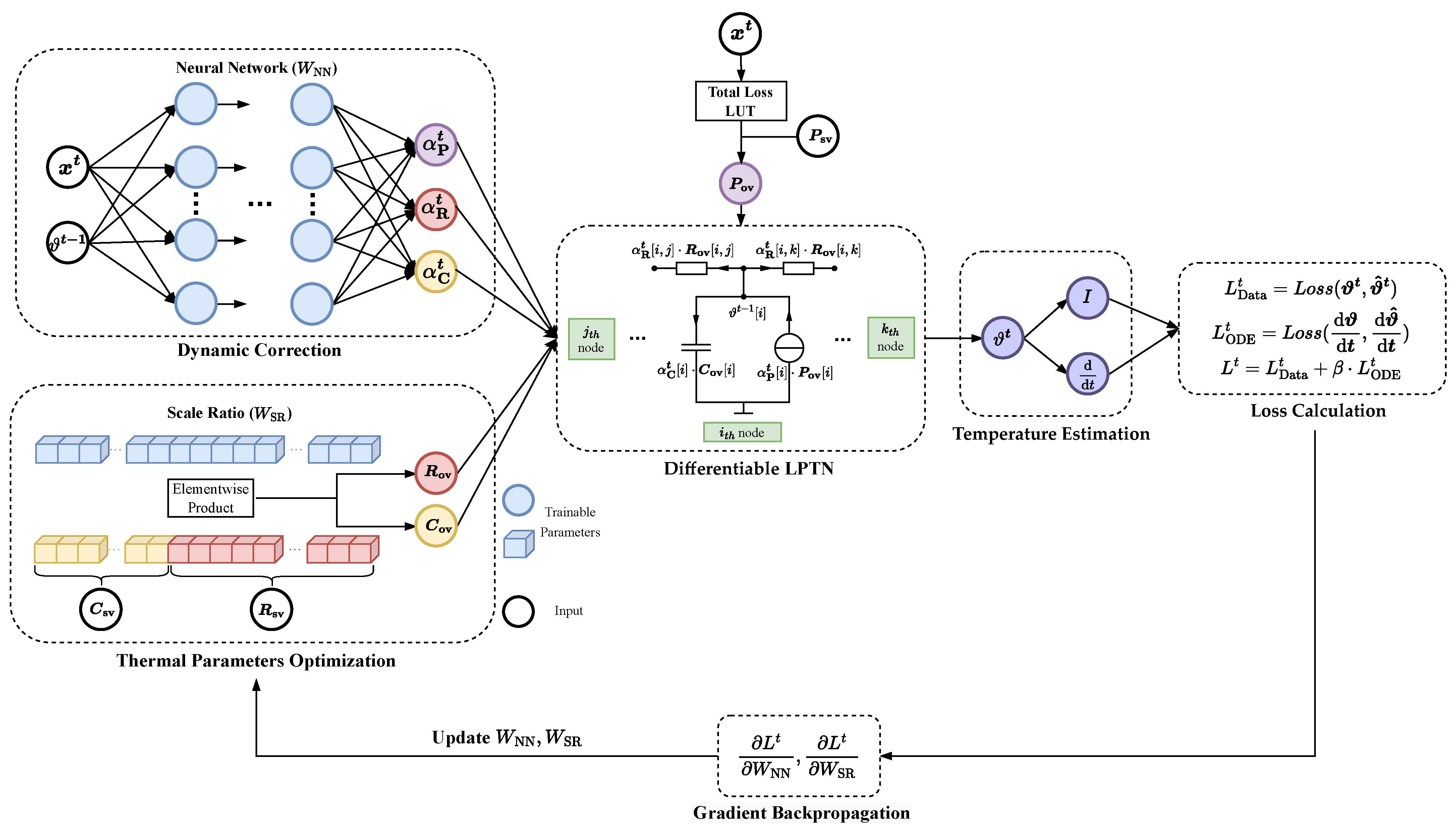
We have implemented a differentiable LPTN in PyTorch and incorporated a neural network to dynamically correct thermal parameters online. The specific estimation framework is shown in Figure 3, which illustrates the flow path to estimate the temperature at each timestep. In general, the raw simulation thermal parameters need to be optimized first to obtain the optimized values that are more in line with the reality (thermal parameter optimization) and then fine-tuned by a neural network to compensate for the relatively small time-varying change (dynamic correction). After that, these thermal parameters are used for solving Equation (2) to obtain the estimated temperatures (differentiable LPTN), which are then transferred to loss calculation and gradient backpropagation during training. A detailed explanation for different components is provided in the following.
4.1. Thermal Parameter Optimization
For a thermal network with n nodes, there typically exist n thermal capacitances, thermal resistances, and less than n thermal losses. These thermal parameters’ simulated values (SVs) exported directly from simulation software, while based on relevant physical theories and empirical formulas, often diverge from their real-world counterparts due to model simplification, the diversity of operating conditions, and environmental impacts. This discrepancy can lead to a decrease in the accuracy of the estimation model. Hence, before directly utilizing these simulated thermal parameters, it is crucial to optimize them to better align with the measured data, which is the key step in enhancing the final estimation accuracy.
Therefore, we add a scaling ratio vector corresponding to thermal capacitances and resistances, which is a learnable parameter, into our framework. By element-wise multiplying simulated values of capacitances and resistances with , we obtain the optimized values (OVs) for these thermal parameters, namely, optimized values of capacitances and resistances . That is,
where the learnable is updated via gradient descent to improve the final temperature estimation accuracy during the training process.
For the simulated values of losses , first, the current operating condition (including speed, torque) is used to determine the total loss based on a lookup table (LUT) derived from real-world motor testing. By normalizing (i.e., element-wise division by the sum) and then multiplying it with total loss, a more accurate is obtained. That is,
4.2. Dynamic Correction
After obtaining the optimized thermal parameters , , and , considering the time-varying characteristic of these parameters, we introduce a neural network into our framework. Taking into account the mechanisms of change and influencing factors of these thermal parameters, the network inputs operating conditions (such as speed, torque, coolant temperature, and ambient temperature) and the estimated temperatures of all nodes at the previous time. Then, it outputs the correction vectors , , and , corresponding to , , and , respectively. The learnable weight is . This step allows for the fine-tuning of the optimized thermal parameters dynamically to improve the final accuracy of temperature estimation. For the i-th node in the lumped parameter thermal network model at time t, its loss , thermal capacity , and thermal resistance between node i and node j are adjusted accordingly, that is,
Using these corrected thermal parameters, the temperature at the next moment can be calculated by Equation (5) and then used for loss calculation as well as gradient backpropagation.
To avoid parameter coupling between and and limit the parameter feasible regions during the actual training of the proposed framework, it is better to conduct the training in two steps. First, the is trained to obtain optimized thermal parameters. This step significantly reduces the temperature estimation error and, due to the fewer learnable parameters of , is unlikely to result in overfitting. Then, the is trained to represent the time-varying characteristics of thermal parameters. At this point, with the error already reduced after the first step, the initial phase of training is less prone to challenges such as gradient explosion, severe fluctuations, or falling into poorly generalized local minima.
4.3. Loss and Backpropagation
The corrected thermal losses, capacitances, and resistances are fed into the subsequent differentiable LPTN to estimate the temperature. The estimated temperature is then compared with the true temperature. Finally, the gradients are backpropagated to update and .
In this work, the loss function includes not only the error between the estimated temperature and the true measured temperature at each time step, denoted as , but also an additional term related to the error between the temperature change rate and , denoted as . This transient characteristic is primarily introduced by thermal capacitances. Therefore, adding this loss term is also beneficial for the training. The weight of these two loss terms is adjusted by the coefficient , i.e., . Different results in different learning curves and accuracy, which is a hyperparameter.
One can see that temperature estimation is essentially an iterative process that requires real-time operating conditions and the temperature information of the previous time. Therefore, the proposed framework in this paper works like a recurrent neural network (RNN). To avoid excessively long sequences that incur gradient explosion or gradient vanishing, we employ truncated backpropagation through time (TBPTT), a method commonly used to train RNN-like networks, to train the proposed framework. As shown in Figure 4. Specifically, we need to manually truncate the temperature sequence into smaller segments and then backpropagate the errors through these segments during training.
5. Simulation
In this section, we first establish a fine-grained simulation model of the PMSM based on MotorCAD. Then, we generate simulation data under various operating conditions to validate the effectiveness of the proposed method. Finally, we investigate the performance and behavior of the framework under different settings through multiple experiments.
5.1. Thermal Simulation Model
The motor investigated in this work is an 8-pole, 48-slot PMSM designed for automotive use. The fundamental geometric and material parameters are presented in Table 1. The motor’s hairpin winding consists of 5 layers, connected in a Y configuration. To establish a corresponding simulation model in MotorCAD software, we first need to specify more detailed actual geometric parameters in the geometry panel, including radial and axial dimensions, for example, stator inner and outer diameters, axial length, slot depth and width, number of layers of permanent magnets, and the length and angle of each layer, shaft diameter, cooling ducts diameter, etc. The configured radial section, axial section, and 3D view are shown in Figure 5.
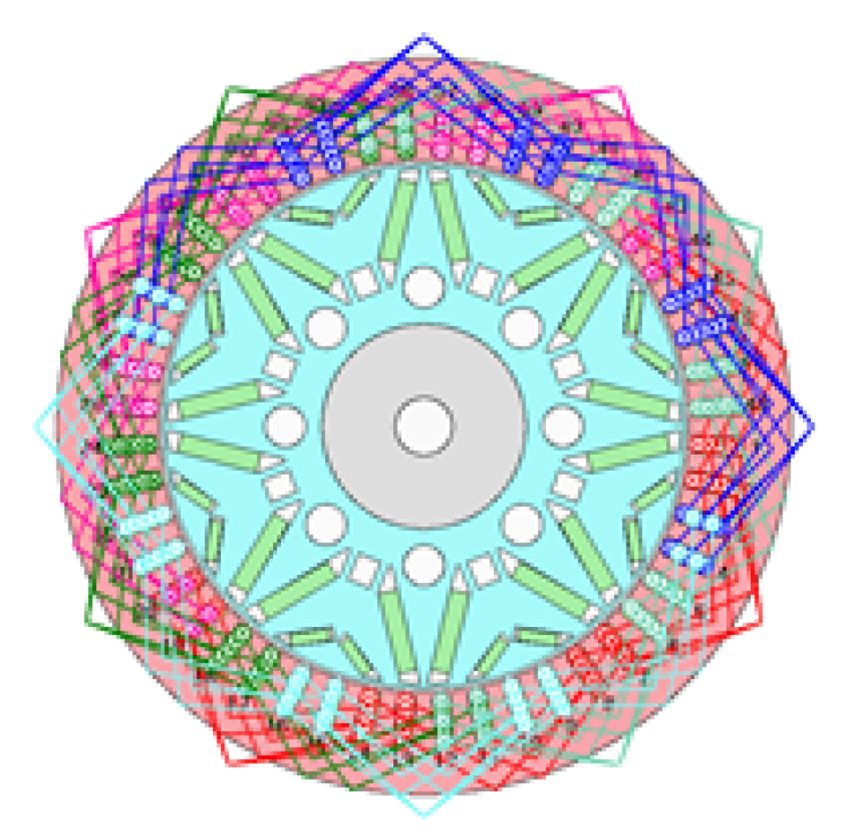
Then, it is necessary to set the specific connection of the winding. The software supports directly selecting hairpin windings and allows customization of the winding connections. The customized winding connections are shown in Figure 6.
By setting the materials of the stator, rotor, and permanent magnets, the software itself provides material-related properties such as thermal conductivity, specific heat, density, etc. For thermal simulation calculations, the cooling of this motor includes housing water jacket cooling, rotor water jacket cooling, and winding end spray, which can be found in Figure 5. The temperature of these coolants is controllable and measurable.
Finally, we can manually formulate duty cycle data for transient temperature calculation. The definitions of duty cycle mainly include torque-speed, loss-speed, and current-speed. When calculating, MotorCAD can build a thermal network based on the actual information of the motor and obtain simulation values for thermal parameters through theoretical and empirical formulas. The fine-grained simulation LPTN includes 135 nodes and is based on the actual geometric parameters, material properties, windings, and cooling system configurations. Subsequently, a simplified thermal model is developed, which consists of 10 nodes, as shown in Figure 7 and Table 2.
Apart from the thermal resistances between the coolant nodes, there are in total 42 thermal resistances. Similarly, the software can provide simulation values for thermal parameters in the simplified thermal model, including torque-speed grid loss data, , and . The torque-speed grid loss data are utilized for obtaining by bilinear interpolation.
5.2. Synthetic Data
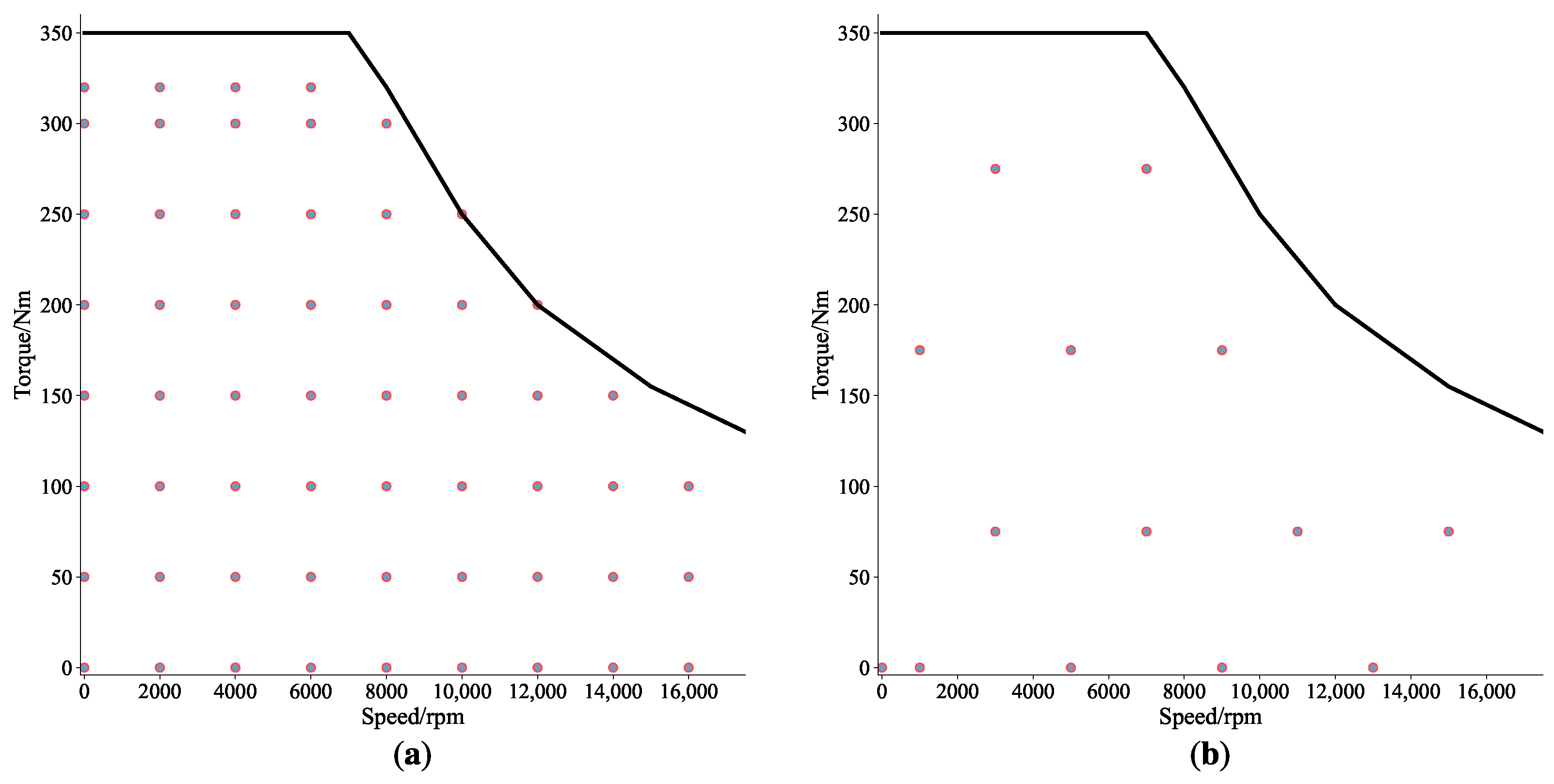
We randomly select from candidate operating points within the motor’s maximum torque/speed curve for constructing a specific set of operating conditions. Subsequently, these conditions are imported into MotorCAD, and the fine-grained thermal model is simulated to obtain temperature data as ground truth. With the simplified thermal model and the corresponding simulation thermal parameters, our proposed method is employed to enhance the temperature estimation accuracy of nodes in the simplified thermal model, thereby validating the effectiveness of our approach. Different sets of candidate operating points are used for generating training and testing conditions to avoid overlap, as indicated by circles in Figure 8.
We finally generated 30 training conditions (20 transient conditions + 10 steady conditions) and 10 testing conditions (5 transient conditions + 5 steady conditions). Each set of conditions has a duration of 800 s and the frequency is 2 Hz.
5.3. Validation Based on Synthetic Data
As described in the previous chapter, firstly, we optimize the simulation thermal parameters that are directly exported from the software with all training data using gradient descent to obtain and . The training process contains 1400 epochs with a small learning rate of 1 × 10⁻⁵ and the error curve during training is shown in Figure 9.
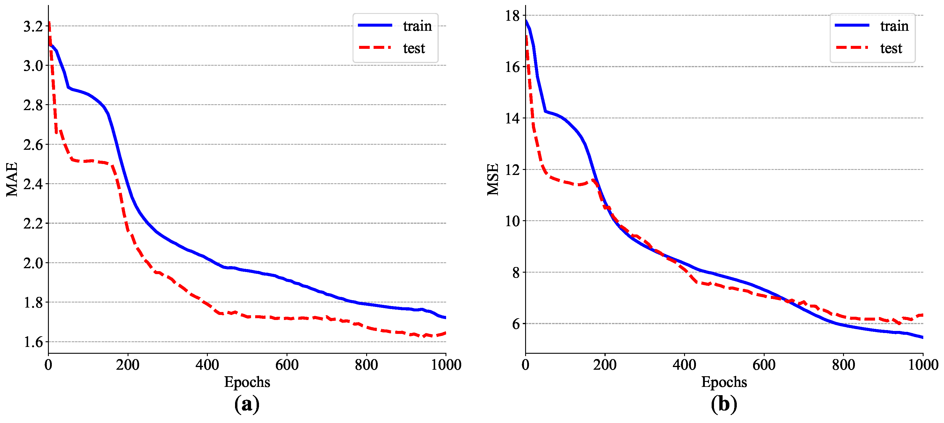
Then, we set the neural network with two hidden layers with sizes of 32 and 64 neurons, respectively, and use Hardswish [28] as the activation function. The optimizer is Adam and initial learning rate is 1 × 10⁻⁴ with cosine annealing decay strategy. The training contains 1200 epochs, with a tbptt size of 1024 and mean squared error (MSE) as loss function. The error curve for the mean absolute error (MAE) and MSE of 7 nodes is as shown in Figure 10.
Figure 11 shows the estimation results of the proposed method. Compared with the results calculated merely based on simulation parameters, it can be seen that the proposed method can achieve excellent accuracy in areas with drastic temperature changes.
To better understand the behaviors of the network, further exploration of model interpretability is conducted. It is meaningful to observe the distribution of correction ratios. Hence, we create a histogram that represents the frequency distribution of correction ratios for all thermal resistances and thermal capacitances in the testing set, as shown in Figure 12 and Table 3. This provides insights into how the corrections are distributed across different components and nodes in the thermal model.
The correction ratios for thermal capacitances are reasonably balanced, showing neither over-correction nor under-correction. The correction magnitudes are relatively small, such as for the stator yoke and rotor. It is also observed that the optimized values for the magnet, Wdg_R, Wdg_A, and tooth are generally larger, leading to correction ratios all less than 1. A similar analysis can be applied to the correction ratios for thermal resistances. The correction magnitudes are mainly distributed between 0.8 and 1.5, indicating subtle rather than drastic adjustments. It is noteworthy that the network actually has the ability to output very small or large correction ratios.
5.4. Ablation Study
Based on synthetic data, we have conducted the following three ablation studies, with the final errors on the testing set shown in Table 4.
5.4.1. The Importance of Simulation Values
We firstly investigated the necessity of , , and , which indicates whether the introduction of simulation values will have an impact on the final temperature estimation accuracy. When making predictions without relying on some simulation values, the network may directly predict values instead of ratios. In this situation, when initializing, the total loss is evenly distributed among the seven nodes. For resistances, considering most of the simulation values are small, all thermal resistances are randomly initialized with a mean of 1/e, and the network’s outputs undergo exponentiation with base e to obtain the final predicted thermal resistances. For capacitances, similarly, the simulation values are in the range of hundreds to thousands, so each node’s thermal capacitance is initialized to around 1200. The outputs of the network need to undergo exponentiation with base 10 to obtain the final predicted thermal capacitances. Such conversion also ensures non-negativity. Furthermore, experiments are conducted under different data sizes, including all data (20 + 10), twelve transient and eight steady conditions (12 + 8), and seven transient and three steady conditions (7 + 3).
5.4.2. Loss Term
For the loss function , the weight of the differential term loss can be adjusted by the coefficient . As mentioned before, the thermal network’s transient characteristics are caused mainly by thermal capacitances. Intuitively, adding a transient-related loss term can benefit the training of the neural network. Therefore, we compare four sets of experiments: , , , and using only . It is important to note that the previous researches are based on . When , the ratio between and is approximately 10:1, and when , it is about 1:1.
5.4.3. Without Correcting One
As shown in Figure 3, considering the time-varying characteristic of thermal parameters, there exists dynamic correction for thermal capacitances, resistances, and losses, respectively, namely, , , and . To examine the impact and necessity of the dynamic correction, the following three different settings are conducted: (1) without correcting capacitances, that is, the capacitances remain unchanged rather than dynamic correction during training and testing; (2) without correcting resistances, that is, the resistances remain unchanged rather than dynamic correction during training and testing; (3) without correcting losses, that is, the losses remain unchanged rather than dynamic correction during training and testing.
6. Experiment
6.1. Bench Testing
We have set up an experimental test bench, as shown in Figure 13. Thermal sensors are used to measure and record temperature data at various positions inside the motor for subsequent validation.
Due to the limitations, we have only measured the three parts of windings (front end, active, and rear end), along with the stator tooth. The internal thermocouple layout scheme is illustrated in Figure 14. There are a total of twenty-four thermocouples, with eight in each layer at the front end and rear end. For the windings in the slot, sensors are placed below the third layer, axially in the middle of the iron core. A total of five thermocouples are arranged for the stator tooth, which are axial in the middle of the iron core.
The acquisition frequency is 10 Hz and the measured temperatures of sensors under a specific operating condition are shown in Figure 15 as an example. It can be observed that the data contain substantial noise. The motor’s placement, cooling conditions, and variations in different winding layers all result in considerable fluctuations in temperature at the same end of windings. We view the average temperature of the sensors in each part of winding as the ground truth, corresponding to Wdg_F, Wdg_A, and Wdg_R.
To obtain more reasonable simulation thermal parameters, this section begins by adjusting the relevant settings of the simulation model. This mainly includes settings related to cooling. The simulation model’s efficiency map is then close to that of the measured motor. At this point, the losses interpolated from the simulation can be considered good initial values for subsequent training. To reduce the computational cost and further alleviate the impact of noise in the high-frequency data, we further downsample the measured data from 10 Hz to 2 Hz. The experimental data were divided into training and testing sets. The training set includes data from nine operating conditions: six steady conditions (continuous performance testing) and three transient conditions (peak performance testing). The testing set includes data from two operating conditions: one steady condition and one transient condition. The total training dataset consists of 46,000 records, similar to the data size of synthetic data. However, it is important to note that the measured data have fewer types of operating points and contain ubiquitous noise, making it more complicated compared to the simulation data.
6.2. Validation Based on Measured Data
6.2.1. The Performance of the Proposed Method
Firstly, to reduce the error of the simulation thermal parameters directly exported by the simulation software, the simulation thermal parameters are optimized using the measured temperature data to obtain optimized values that better align with the measured data. Given the presence of noise in the data, a smaller learning rate and fewer training epochs are used. In this experiment, a learning rate of and 150 epochs with SGD are used.
Then, due to the limited amount of data, especially the limited variety of data types, the number of neurons in the second hidden layer of the network is reduced to 32. Considering that the network can output temperatures for seven nodes but only label data for three nodes are provided, this essentially constitutes an under-constrained optimization problem. The previous section shows that the dynamic correction is merely fine-tuning optimized thermal parameters. Therefore, we artificially restrict the magnitude range of , , and . This also highlights one of the advantages brought by incorporating simulation parameters. Additionally, it is important to note that we do not utilize any normalization layers that are commonly used in deep learning, such as LayerNorm [29] or BatchNorm [30]. It is because after normalization, the original physical meaning of an input cannot be preserved. For instance, different physical quantities like speed or torque may be mapped to the same value after normalization, therefore losing comparability between two operating points. This contradicts the principles of physical mechanisms, brings severe fluctuations, and affects the final accuracy, despite speeding up the training speed in the early and middle stages through our experiments.
We use Adam for 1000 epochs and the initial learning rate is . The tbptt size remains 1024. Since we almost remove outliers during the data processing stage, we use mse loss, which is helpful for reducing the maximum error. The average error during training and the final accuracy is shown in Figure 16 and Table 5. The temperature estimation results on the test conditions are shown in Figure 17.
6.2.2. Method Comparison
We have compared two common models in time-series regression prediction with comparable number of learnable parameters, namel, long short-term memory (LSTM) and temporal convolutional network (TCN). Additional steps such as data standardization and feature engineering are performed for these two. Referring to reference [31], the exponential moving average (EWMA) and exponential moving average standard deviation (EWMS) are calculated for speed, torque, current, voltage, power, and coolant temperature with window sizes of 200, 400, resulting in a total of 22 features. It is noteworthy that the proposed physics-based temperature estimation framework only requires speed, torque, and coolant temperature, without the need for any feature engineering. However, for LSTM and TCN, we found that without feature engineering, comparable prediction results could not be achieved with such a small dataset. We manually choose specific hyperparameters to achieve better accuracy for both algorithms, which are shown in Table 6.
The final prediction accuracy is compared with the results of the proposed method in Table 7. It can be observed from Figure 18 that both models have enough fitting capability, achieving very low errors on the training set. However, they show a significant overfitting, as evidenced by the noticeable gap in accuracy on the testing set and a relatively large maximum error. Notably, LSTM performs worse than TCN, possibly due to TCN’s ability to better capture both local and global patterns in the data.
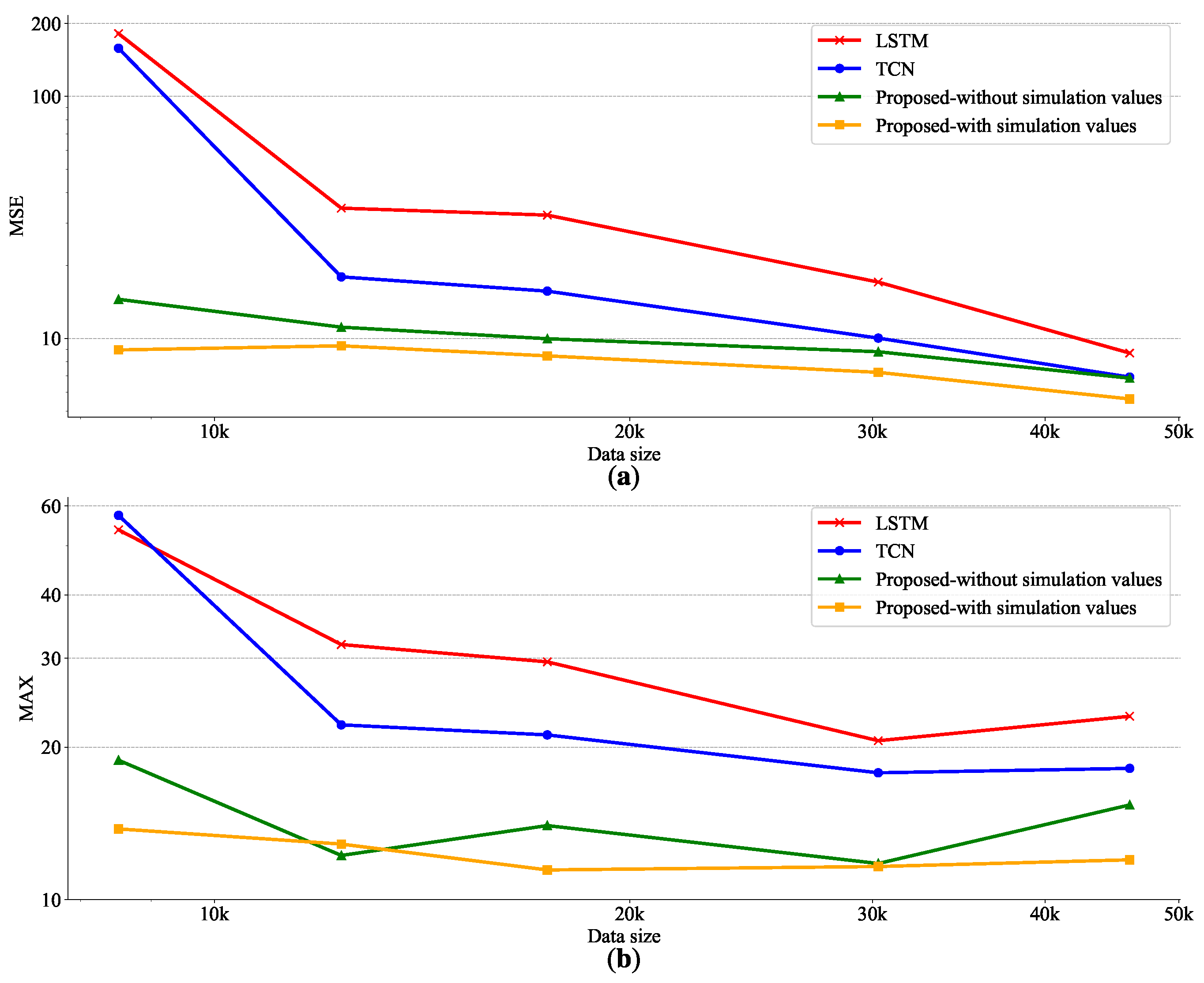
Next, we investigate the impact of data size on the accuracy of different methods, as shown in Figure 19 and Table 8. The variation in accuracy under different data sizes can effectively examine the robustness and stability of different methods.
It can be observed that the proposed method consistently achieves better results, regardless of whether based on simulation values or not. The accuracy remains relatively stable with varying data size. In contrast, the accuracy of data-driven algorithms undergoes a significant decline, although they still perform well on the training set. Considering both mean squared error and maximum error, the proposed method obtains the best results with minimal sensitivity to data size. Due to the incorporation of physical priors and physical constraints, the proposed method is less dependent on data and more effective in extracting information contained within the data.
6.3. The Temperature Estimation of Stator Tooth
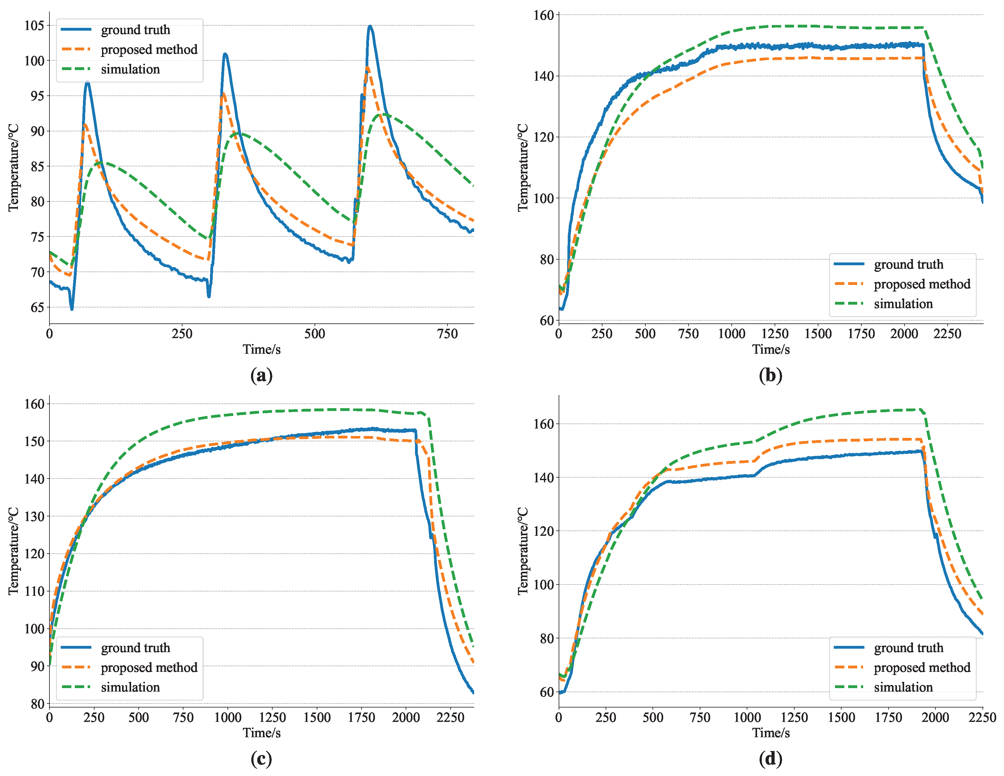
This section explores the estimation result for the stator tooth under different settings. Since the proposed method can simultaneously output temperatures for all nodes, this analysis serves as an extension to validate the framework and an example to demonstrate the potential application. The stator tooth’s temperature data are not involved in the training, making the tooth’s temperature in the training set also suitable for evaluating the final performance. Figure 20 illustrates the estimated tooth’s temperature obtained by the proposed method with simulation thermal parameters for four different operating conditions. It is noteworthy that even without providing any measured data of the tooth, the framework, guided by the thermal network structure and physical priors, achieves considerable accuracy in estimating the temperature of tooth.
Table 9 further illustrates the estimation results when not based on some SVs. It is worth noting that these models all exhibit relatively small errors on three winding nodes. However, when discarding or when no simulation values are used at all, the estimation errors become significantly large. It should be pointed out that, if relying solely on the simulation thermal parameters and without considering dynamic correction, the corresponding tooth temperature estimation errors MAE, MSE, and MAX are 9.34 °C, 119.83 °C2, and 29.22 °C, respectively. The neural network trained with three SVs achieves the highest accuracy, followed by without , as the number of thermal capacitances is small and the given initial values are relatively reasonable. However, when all SVs are not provided, the estimated tooth temperature is essentially meaningless.
7. Discussion
Previous studies have largely focused on either purely data-driven methods or models heavily reliant on physical principles without integrating the advantages of machine learning techniques. This paper proposes a temperature estimation framework that integrates physical information with data-driven methods. The proposed framework effectively combines neural networks, differentiable physical models, and simulation results and addresses the limitations of purely data-driven methods (lack of physical interpretability and potential divergence from physical principles) and purely physical models (rigidity and potential inaccuracies in modeling complex real-world phenomena). The effectiveness of this method is validated by using both synthetic data and measured data, including a thorough ablation study of various settings, diverse comparisons with common data-driven methods, and the exploration of temperature estimation for the node without any associated labels. Due to the incorporation of physical principles, the output temperatures are more reasonable and robust, and the overall results exhibit better physical consistency. This method holds significant practical value and is crucial for optimizing motor performance, extending lifespan, and ensuring safety in applications where thermal management is critical.
While the current findings are promising, several future research directions can further enhance the framework’s applicability:
- Validating the proposed method’s effectiveness and generalization ability by utilizing a more extensive and diverse set of real-world data;
- Investigating other neural network architectures, such as graphic neural networks (GNNs) or convolutional neural networks (CNNs), could provide insights into their efficacy in capturing temporal dynamics and spatial relationships within motor systems;
- Implementing the framework in real-time control systems and validating its performance in operational environments would be a crucial step toward its industrial application.
Author Contributions
Conceptualization, P.W., X.W. and Y.W.; methodology, P.W., X.W. and Y.W.; software, P.W.; validation, P.W.; formal analysis, P.W. and X.W.; investigation, P.W., X.W. and Y.W.; resources, Y.W.; data curation, P.W. and X.W.; writing—original draft preparation, P.W., X.W. and Y.W.; writing—review and editing, P.W., X.W. and Y.W.; visualization, P.W. and X.W.; supervision, X.W. and Y.W.; project administration, X.W. and Y.W. All authors have read and agreed to the published version of the manuscript.
Funding
This research received no external funding.
Data Availability Statement
The datasets presented in this study are available on request from the corresponding author due to privacy.
Conflicts of Interest
Yunpeng Wang is an employee of Leadrive Technology. The paper reflects the views of the scientists and not the company.
References
- Ilie, S.; Toader, D.; Barvinschi, F. Modern education on renewable energies by using numerical Finite Element Method of a solar powered Stirling engine with heat transfer simulations. In Proceedings of the 2016 12th IEEE International Symposium on Electronics and Telecommunications (ISETC), Timisoara, Romania, 27–28 October 2016; pp. 137–140. [Google Scholar]
- Ruoho, S.; Kolehmainen, J.; Ikaheimo, J.; Arkkio, A. Interdependence of demagnetization, loading, and temperature rise in a permanent-magnet synchronous motor. IEEE Trans. Magn. 2009, 46, 949–953. [Google Scholar] [CrossRef]
- Ganchev, M.; Kubicek, B.; Kappeler, H. Rotor temperature monitoring system. In Proceedings of the XIX International Conference on Electrical Machines—ICEM 2010, Rome, Italy, 6–8 September 2010; pp. 1–5. [Google Scholar]
- Mejuto, C.; Mueller, M.; Shanel, M.; Mebarki, A.; Reekie, M.; Staton, D. Improved synchronous machine thermal modelling. In Proceedings of the 2008 18th International Conference on Electrical Machines, Vilamoura, Portugal, 6–9 September 2008; pp. 1–6. [Google Scholar]
- Specht, A.; Wallscheid, O.; Böcker, J. Determination of rotor temperature for an interior permanent magnet synchronous machine using a precise flux observer. In Proceedings of the 2014 International Power Electronics Conference (IPEC—Hiroshima 2014—ECCE ASIA), Hiroshima, Japan, 18–21 May 2014; pp. 1501–1507. [Google Scholar]
- Fernandez, D.; Hyun, D.; Park, Y.; Reigosa, D.D.; Lee, S.B.; Lee, D.M.; Briz, F. Permanent magnet temperature estimation in PM synchronous motors using low-cost hall effect sensors. IEEE Trans. Ind. Appl. 2017, 53, 4515–4525. [Google Scholar] [CrossRef]
- Ganchev, M.; Kral, C.; Oberguggenberger, H.; Wolbank, T. Sensorless rotor temperature estimation of permanent magnet synchronous motor. In Proceedings of the IECON 2011—37th Annual Conference of the IEEE Industrial Electronics Society, Melbourne, VIC, Australia, 7–10 November 2011; pp. 2018–2023. [Google Scholar]
- Reigosa, D.D.; Briz, F.; García, P.; Guerrero, J.M.; Degner, M.W. Magnet temperature estimation in surface PM machines using high-frequency signal injection. IEEE Trans. Ind. Appl. 2010, 46, 1468–1475. [Google Scholar] [CrossRef]
- Qi, F.; Schenk, M.; De Doncker, R. Discussing details of lumped parameter thermal modeling in electrical machines. In Proceedings of the 7th IET International Conference on Power Electronics, Machines and Drives (PEMD 2014), Manchester, UK, 8–10 April 2014. [Google Scholar]
- Wallscheid, O.; Huber, T.; Peters, W.; Böcker, J. Real-time capable methods to determine the magnet temperature of permanent magnet synchronous motors—A review. In Proceedings of the IECON 2014—40th Annual Conference of the IEEE Industrial Electronics Society, Dallas, TX, USA, 29 October–1 November 2014; pp. 811–818. [Google Scholar]
- Dilshad, M.; Ashok, S.; Vijayan, V.; Pathiyil, P. An energy loss model based temperature estimation for Permanent Magnet Synchronous Motor (PMSM). In Proceedings of the 2016 2nd International Conference on Advances in Electrical, Electronics, Information, Communication and Bio-Informatics (AEEICB), Chennai, India, 27–28 February 2016; pp. 172–176. [Google Scholar]
- Park, J.B.; Moosavi, M.; Toliyat, H.A. Electromagnetic-thermal coupled analysis method for interior PMSM. In Proceedings of the 2015 IEEE International Electric Machines & Drives Conference (IEMDC), Seattle, WA, USA, 10–13 May 2015; pp. 1209–1214. [Google Scholar]
- Choi, J.; Lee, J.; Ha, J.I. Stator Temperature Estimation of PMSM Based on Thermal Equivalent Circuit. In Proceedings of the 2019 22nd International Conference on Electrical Machines and Systems (ICEMS), Harbin, China, 11–14 August 2019; pp. 1–4. [Google Scholar]
- Wallscheid, O.; Böcker, J. Global identification of a low-order lumped-parameter thermal network for permanent magnet synchronous motors. IEEE Trans. Energy Convers. 2015, 31, 354–365. [Google Scholar] [CrossRef]
- Wallscheid, O.; Kirchgässner, W.; Böcker, J. Investigation of long short-term memory networks to temperature prediction for permanent magnet synchronous motors. In Proceedings of the 2017 International Joint Conference On Neural Networks (IJCNN), Anchorage, AK, USA, 14–19 May 2017; pp. 1940–1947. [Google Scholar]
- Kirchgässner, W.; Wallscheid, O.; Böcker, J. Estimating electric motor temperatures with deep residual machine learning. IEEE Trans. Power Electron. 2020, 36, 7480–7488. [Google Scholar] [CrossRef]
- Lee, J.; Ha, J.I. Temperature estimation of PMSM using a difference-estimating feedforward neural network. IEEE Access 2020, 8, 130855–130865. [Google Scholar] [CrossRef]
- Raissi, M.; Perdikaris, P.; Karniadakis, G.E. Physics-informed neural networks: A deep learning framework for solving forward and inverse problems involving nonlinear partial differential equations. J. Comput. Phys. 2019, 378, 686–707. [Google Scholar] [CrossRef]
- Karniadakis, G.E.; Kevrekidis, I.G.; Lu, L.; Perdikaris, P.; Wang, S.; Yang, L. Physics-informed machine learning. Nat. Rev. Phys. 2021, 3, 422–440. [Google Scholar] [CrossRef]
- Thuerey, N.; Holl, P.; Mueller, M.; Schnell, P.; Trost, F.; Um, K. Physics-based deep learning. arXiv 2021, arXiv:2109.05237. [Google Scholar]
- Seo, S.; Liu, Y. Differentiable physics-informed graph networks. arXiv 2019, arXiv:1902.02950. [Google Scholar]
- Qiao, Y.L.; Liang, J.; Koltun, V.; Lin, M.C. Scalable differentiable physics for learning and control. arXiv 2020, arXiv:2007.02168. [Google Scholar]
- Veg, L.; Laksar, J. Thermal model of high-speed synchronous motor created in MATLAB for fast temperature check. In Proceedings of the 2018 18th International Conference on Mechatronics-Mechatronika (ME), Brno, Czech Republic, 5–7 December 2018; pp. 1–5. [Google Scholar]
- Wallscheid, O.; Böcker, J. Design and identification of a lumped-parameter thermal network for permanent magnet synchronous motors based on heat transfer theory and particle swarm optimisation. In Proceedings of the 2015 17th European Conference on Power Electronics and Applications (EPE’15 ECCE-Europe), Geneva, Switzerland, 8–10 September 2015; pp. 1–10. [Google Scholar]
- Kirchgässner, W.; Wallscheid, O.; Böcker, J. Thermal neural networks: Lumped-parameter thermal modeling with state-space machine learning. Eng. Appl. Artif. Intell. 2023, 117, 105537. [Google Scholar] [CrossRef]
- Wang, P.; Wang, X.; Wang, Y. Physics-Informed Machine Learning Based Permanent Magnet Synchronous Motor Temperature Estimation. In Proceedings of the 2023 International Conference on Mechanical and Electronics Engineering (ICMEE), Xi’an, China, 17–19 November 2023; pp. 582–587. [Google Scholar]
- Bergman, T.L. Fundamentals of Heat and Mass Transfer; John Wiley & Sons: Hoboken, NJ, USA, 2011. [Google Scholar]
- Howard, A.; Sandler, M.; Chu, G.; Chen, L.C.; Chen, B.; Tan, M.; Wang, W.; Zhu, Y.; Pang, R.; Vasudevan, V.; et al. Searching for mobilenetv3. In Proceedings of the IEEE/CVF International Conference on Computer Vision, Seoul, Republic of Korea, 27 October–2 November 2019; pp. 1314–1324. [Google Scholar]
- Ba, J.L.; Kiros, J.R.; Hinton, G.E. Layer normalization. arXiv 2016, arXiv:1607.06450. [Google Scholar]
- Ioffe, S.; Szegedy, C. Batch normalization: Accelerating deep network training by reducing internal covariate shift. In Proceedings of the International Conference on Machine Learning, Lille, France, 7–9 July 2015; pp. 448–456. [Google Scholar]
- Kirchgässner, W.; Wallscheid, O.; Böcker, J. Empirical evaluation of exponentially weighted moving averages for simple linear thermal modeling of permanent magnet synchronous machines. In Proceedings of the 2019 IEEE 28th International Symposium on Industrial Electronics (ISIE), Vancouver, BC, Canada, 12–14 June 2019; pp. 318–323. [Google Scholar]
Figure 1.
Different ways of combining physical models with neural networks. (a) Neural networks first; (b) physical models first; (c) parallel. For (a), the output of the neural network is fed into the following physical model. For (b) and (c), the gradients generally do not directly flow through the physical model, and the neural network primarily serves to learn the residual error.

Figure 2.
The i-th node in a typical LPTN.

Figure 3.
Differentiable physics temperature estimation framework. (1) Thermal parameter optimization: simulation thermal parameters are optimized to obtain better initial values. (2) Dynamic correction: the neural network predicts several correction ratios at each time step. These two outputs are then fed into the downstream differentiable thermal model to obtain the estimated temperature.

Figure 4.
Truncated backpropagation through time (TBPTT) for training the proposed framework.

Figure 5.
Simulation model in MotorCAD. (a) Radial section; (b) axial section; (c) 3D view. Different colors represent different components of the motor, while the arrows in (b) and (c) denote the cooling paths in the simulation model.
Figure 5.
Simulation model in MotorCAD. (a) Radial section; (b) axial section; (c) 3D view. Different colors represent different components of the motor, while the arrows in (b) and (c) denote the cooling paths in the simulation model.

Figure 6.
Hairpin winding of simulation model.

Figure 7.
Simplified thermal model (10 nodes). For better visualization, we only display the distribution of several thermal resistances.
Figure 7.
Simplified thermal model (10 nodes). For better visualization, we only display the distribution of several thermal resistances.

Figure 8.
Candidate points (represented by circles) for constituting operating conditions. (a) Training; (b) testing. For both training and testing conditions, choose non-overlapping operating points.
Figure 8.
Candidate points (represented by circles) for constituting operating conditions. (a) Training; (b) testing. For both training and testing conditions, choose non-overlapping operating points.

Figure 9.
The error curve for optimizing the simulation thermal parameters, which are directly exported from the software. This step corresponds to thermal parameter optimization in Figure 3.
Figure 9.
The error curve for optimizing the simulation thermal parameters, which are directly exported from the software. This step corresponds to thermal parameter optimization in Figure 3.

Figure 10.
Error curve during training. (a) MAE; (b) MSE.

Figure 11.
The performance of the proposed method on synthetic data. (a) Stator yoke temperature estimation result; (b) stator yoke temperature estimation error; (c) Wdg_R temperature estimation result; (d) Wdg_R temperature estimation error.
Figure 11.
The performance of the proposed method on synthetic data. (a) Stator yoke temperature estimation result; (b) stator yoke temperature estimation error; (c) Wdg_R temperature estimation result; (d) Wdg_R temperature estimation error.

Figure 12.
The frequency distribution of correction ratios for thermal capacitances and thermal resistances. (a) Capacitances; (b) resistances.
Figure 12.
The frequency distribution of correction ratios for thermal capacitances and thermal resistances. (a) Capacitances; (b) resistances.

Figure 13.
Motor test bench.

Figure 14.
Arrangement of thermal sensors at the winding. (a) U-shaped winding; (b) axial middle in slots; (c) welded winding. 8 sensors for each layer at the U-shaped end and welding end; 5 sensors for the third layer at the axial middle in slots.
Figure 14.
Arrangement of thermal sensors at the winding. (a) U-shaped winding; (b) axial middle in slots; (c) welded winding. 8 sensors for each layer at the U-shaped end and welding end; 5 sensors for the third layer at the axial middle in slots.

Figure 15.
Temperature curves measured by all thermal sensors at four different locations. (a) U-shaped (24 thermocouples); (b) welded (24 thermocouples); (c) axial middle (5 thermocouples); (d) tooth (3 thermocouples).
Figure 15.
Temperature curves measured by all thermal sensors at four different locations. (a) U-shaped (24 thermocouples); (b) welded (24 thermocouples); (c) axial middle (5 thermocouples); (d) tooth (3 thermocouples).

Figure 16.
The error curve during training. (a) MAE; (b) MSE.

Figure 17.
The temperature estimation results of the test conditions of the proposed method. (a) Wdg_F; (b) Wdg_A; (c) Wdg_R; (d) Wdg_F; (e) Wdg_A; (f) Wdg_R. (a–c) correspond to the same operating condition; (d–f) correspond to another operating condition.
Figure 17.
The temperature estimation results of the test conditions of the proposed method. (a) Wdg_F; (b) Wdg_A; (c) Wdg_R; (d) Wdg_F; (e) Wdg_A; (f) Wdg_R. (a–c) correspond to the same operating condition; (d–f) correspond to another operating condition.

Figure 18.
The error curves of LSTM and TCN during training. (a) LSTM; (b) TCN.

Figure 19.
The mean square error and max error on the testing set when providing different numbers of training data. The testing set remains unchanged. (a) MSE; (b) MAX.
Figure 19.
The mean square error and max error on the testing set when providing different numbers of training data. The testing set remains unchanged. (a) MSE; (b) MAX.

Figure 20.
Estimation results for stator tooth temperature. (a–d) are four different operating conditions.
Figure 20.
Estimation results for stator tooth temperature. (a–d) are four different operating conditions.


Table 1.
Parameters of the permanent magnet synchronous motor in this work.
| Parameter | Value |
|---|---|
| Slot Number | 48 |
| Pole Number | 8 |
| Housing Outer Diameter | 206 mm |
| Stator Outer Diameter | 180 mm |
| Stator Inner Diameter | 130 mm |
| Shaft Diameter | 50 mm |
| Air Gap | 1 mm |
| Slot Width | 4.6 mm |
| Slot Depth | 13.62 mm |
| Motor Length | 250 mm |
| Stator Length | 135 mm |
| Peak Torque | ≥345 Nm |
| Maximum Rotating Speed | 20,000 rpm |
| Peak Power | ≥245 kW @ 650 Vdc |
Table 2.
The meaning of each node in the simplified thermal model.
| Node Name | Meaning |
|---|---|
| Stator Yoke | Stator yoke |
| Wdg_F | Front end of the third-layer winding |
| Wdg_A | Active of the third-layer winding |
| Wdg_R | Rear end of the third-layer winding |
| Tooth | Third-layer stator tooth |
| Rotor | Rotor core |
| Magnet | Permanent magnet |
| Housing Coolant * | Housing cooling inlet |
| Rotor Coolant * | Rotor cooling inlet |
| Ambient * | Ambient |
* The temperatures of these nodes are known at each time.
Table 3.
The range of correction scale ratio for each node.
| Stator Yoke | Magnet | Rotor | Wdg_F | Wdg_R | Wdg_A | Tooth |
|---|---|---|---|---|---|---|
| (0.87, 1.07) | (0.25, 0.78) | (1.11, 1.22) | (0.79, 1.21) | (0.85, 1.00) | (0.57, 0.96) | (0.58, 1.00) |
Table 4.
Ablation study based on synthetic data. MAE: mean absolute error; MSE: mean square error; MAX: maximum error.
Table 4.
Ablation study based on synthetic data. MAE: mean absolute error; MSE: mean square error; MAX: maximum error.
| Additional Conditions | MAE | MSE | MAX | |||
|---|---|---|---|---|---|---|
| × | √ | √ | - | 0.77 | 1.18 | 7.71 |
| √ | × | √ | - | 0.97 | 3.13 | 8.91 |
| √ | √ | × | - | 1.85 | 11.59 | 20.68 |
| × | × | × | - | 1.34 | 4.40 | 12.37 |
| √ | √ | √ | - | 0.80 | 1.21 | 5.25 |
| × | × | × | 12 + 8 | 1.33 | 4.99 | 14.00 |
| √ | √ | √ | 12 + 8 | 0.89 | 1.63 | 11.17 |
| × | × | × | 7 + 3 | 1.85 | 9.94 | 15.34 |
| √ | √ | √ | 7 + 3 | 0.98 | 2.02 | 8.21 |
| √ | √ | √ | 0.79 | 1.20 | 5.16 | |
| √ | √ | √ | 0.77 | 1.16 | 4.84 | |
| √ | √ | √ | only | 1.25 | 3.17 | 9.09 |
| √ | √ | √ | w/o correcting capacitances | 0.96 | 1.83 | 6.23 |
| √ | √ | √ | w/o correcting resistances | 2.23 | 18.96 | 30.16 |
| √ | √ | √ | w/o correcting losses | 1.20 | 4.14 | 15.23 |
Table 5.
Ablation study based on measured data.
| Additional Conditions | MAE | MSE | MAX | |||
|---|---|---|---|---|---|---|
| × | √ | √ | - | 1.93 | 7.15 | 15.46 |
| √ | × | √ | - | 1.91 | 6.96 | 13.80 |
| √ | √ | × | - | 1.98 | 7.04 | 12.69 |
| × | × | × | - | 1.97 | 6.85 | 15.38 |
| √ | √ | √ | - | 1.64 | 6.33 | 13.75 |
| √ | √ | √ | 1.57 | 5.62 | 11.98 | |
| √ | √ | √ | 2.01 | 7.65 | 11.46 | |
| √ | √ | √ | w/o correcting capacitances | 1.96 | 7.68 | 15.98 |
| √ | √ | √ | w/o correcting resistances | 2.32 | 9.79 | 15.92 |
| √ | √ | √ | w/o correcting losses | 2.26 | 10.82 | 18.44 |
Table 6.
Hyperparameters corresponding to LSTM and TCN.
| Hyperparameters | LSTM | TCN |
|---|---|---|
| Hidden Neurons | 16 | 16 |
| Stacking Layers | 1 | 1 |
| Optimizer | Adam | |
| Epochs | 1500 | |
| Learning Rate | 0–1300: , 1300–1500: | |
| TBPTT Size | 512 | - |
| Dropout | - | 0.2 |
| Kernel Size | - | 3 |
| Learnable Parameters | 2.6 k | 2.3 k |
Table 7.
The error of different methods.
| TCN | LSTM | Proposed | |
|---|---|---|---|
| MAE | 2.47 | 2.55 | 1.57 |
| MSE | 6.92 | 8.70 | 5.62 |
| MAX | 18.16 | 23.02 | 11.98 |
Table 8.
The errors on the testing set when different amounts of training data are provided. w/o values and w values mean the proposed method without and with simulation values.
Table 8.
The errors on the testing set when different amounts of training data are provided. w/o values and w values mean the proposed method without and with simulation values.
| Method | 46k | 30k | 17k | 12k | 8k | |
|---|---|---|---|---|---|---|
| MSE | LSTM | 8.70 | 17.09 | 32.33 | 34.54 | 181.81 |
| TCN | 6.96 | 10.11 | 15.57 | 17.88 | 158.21 | |
| w/o values | 6.85 | 8.81 | 9.89 | 11.13 | 14.51 | |
| w values | 5.62 | 7.21 | 8.47 | 9.32 | 8.96 | |
| MAX | LSTM | 23.02 | 20.60 | 29.49 | 31.91 | 53.77 |
| TCN | 18.16 | 17.78 | 21.15 | 22.14 | 57.44 | |
| w/o values | 15.38 | 11.80 | 14.00 | 12.22 | 18.85 | |
| w values | 11.98 | 11.62 | 11.44 | 12.87 | 13.79 |
Table 9.
The estimation errors for stator tooth temperature.
| w Values | w/o | w/o | w/o | w/o Values | |
|---|---|---|---|---|---|
| MAE | 4.59 | 4.78 | 39.33 | 11.87 | 51.63 |
| MSE | 29.84 | 33.20 | 2421.97 | 233.75 | 4146.79 |
| MAX | 18.39 | 23.12 | 117.46 | 86.02 | 288.13 |
Disclaimer/Publisher’s Note: The statements, opinions and data contained in all publications are solely those of the individual author(s) and contributor(s) and not of MDPI and/or the editor(s). MDPI and/or the editor(s) disclaim responsibility for any injury to people or property resulting from any ideas, methods, instructions or products referred to in the content. |
© 2024 by the authors. Licensee MDPI, Basel, Switzerland. This article is an open access article distributed under the terms and conditions of the Creative Commons Attribution (CC BY) license (https://creativecommons.org/licenses/by/4.0/).
Share and Cite
MDPI and ACS Style
Wang, P.; Wang, X.; Wang, Y. End-to-End Differentiable Physics Temperature Estimation for Permanent Magnet Synchronous Motor. World Electr. Veh. J. 2024, 15, 174. https://doi.org/10.3390/wevj15040174
AMA Style
Wang P, Wang X, Wang Y. End-to-End Differentiable Physics Temperature Estimation for Permanent Magnet Synchronous Motor. World Electric Vehicle Journal. 2024; 15(4):174. https://doi.org/10.3390/wevj15040174
Chicago/Turabian StyleWang, Pengyuan, Xinjian Wang, and Yunpeng Wang. 2024. "End-to-End Differentiable Physics Temperature Estimation for Permanent Magnet Synchronous Motor" World Electric Vehicle Journal 15, no. 4: 174. https://doi.org/10.3390/wevj15040174