Appendix A
Figure A1.
Comparison EMSP- and CPO-dataset of Munich regarding connection duration and transmitted energy of AC and DC charging events.
Figure A1.
Comparison EMSP- and CPO-dataset of Munich regarding connection duration and transmitted energy of AC and DC charging events.
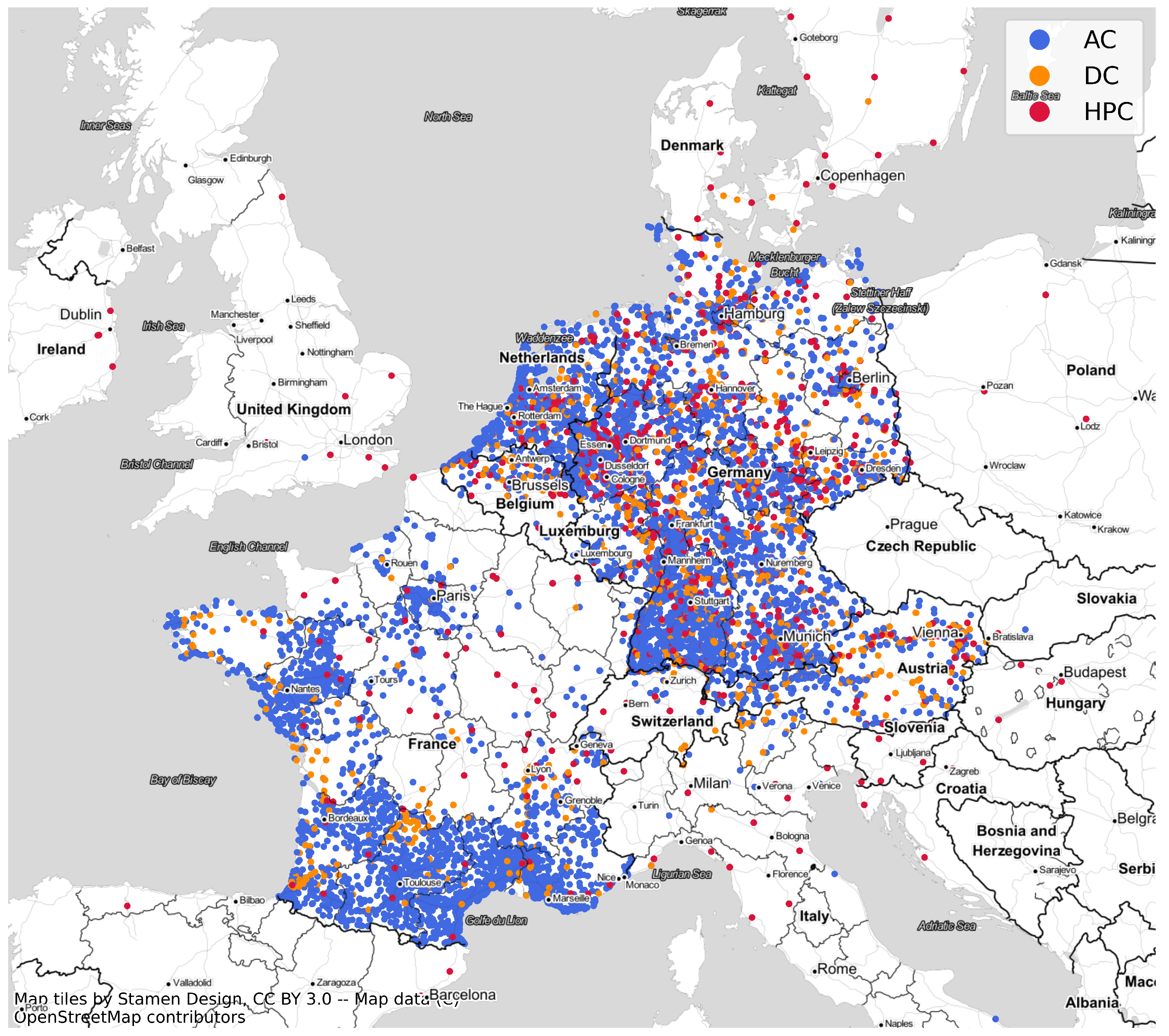
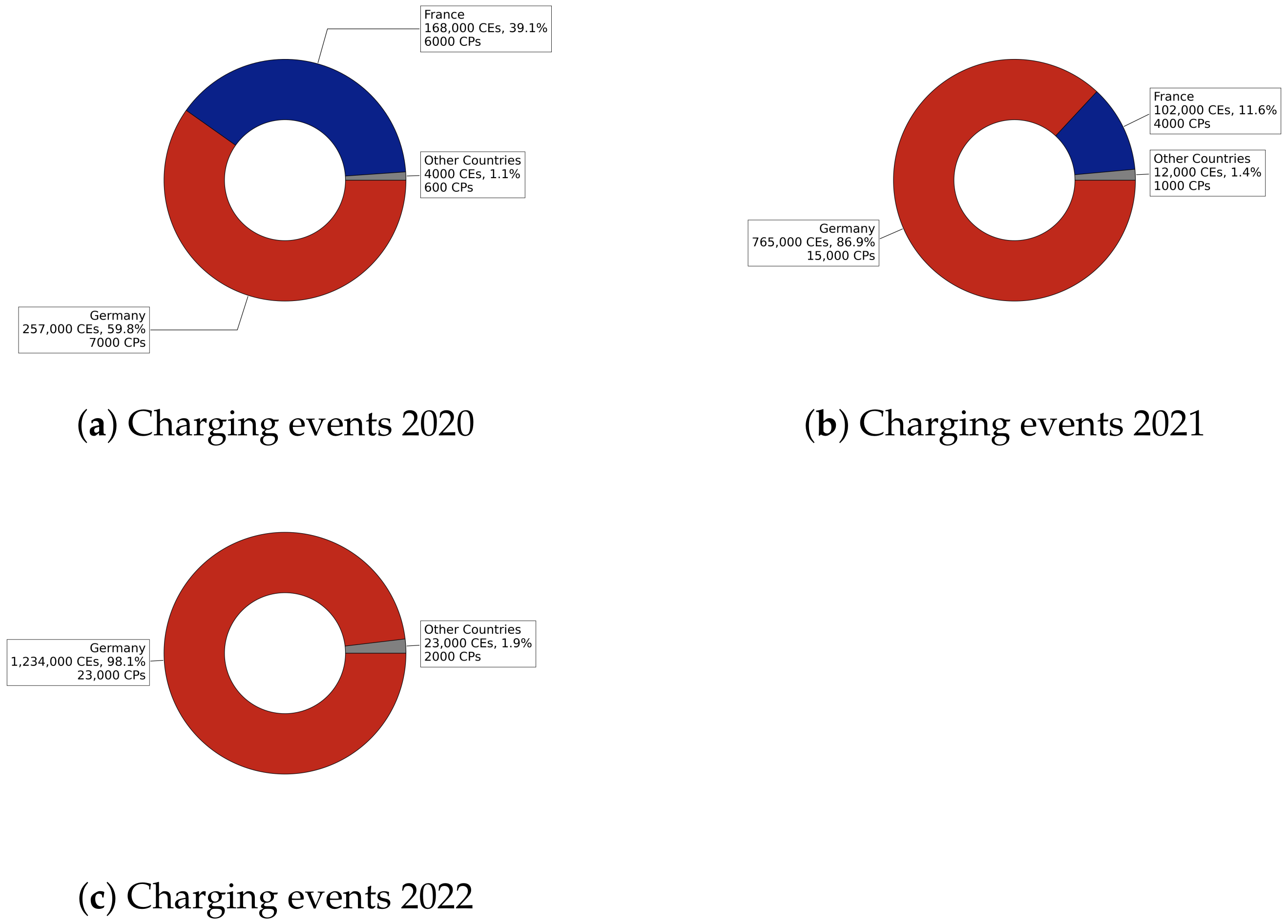
Figure A2.
Number of charging events per country and period of time in the dataset.
Figure A2.
Number of charging events per country and period of time in the dataset.
Table A1.
KPIs of AC charging events from the real-world dataset per country.
Table A1.
KPIs of AC charging events from the real-world dataset per country.
| Country | Number of CPs | Number of CEs | Power Range [kW] | Avg./Median Con. Duration [h/CE] | Avg./Median Energy [kWh/CE] |
|---|
| Germany | 20,000 | 2 m | 3–43 | 4.9/3.1 | 14.8/10.5 |
| France | 5900 | 240,600 | 3–43 | 4.2/2.2 | 18.8/15.2 |
Table A2.
KPIs of DC charging events from the real-world dataset per country.
Table A2.
KPIs of DC charging events from the real-world dataset per country.
| Country | Number of CPs | Number of CEs | Power Range [kW] | Avg./Median Con. Duration [h/CE] | Avg./Median Energy [kWh/CE] |
|---|
| Germany | 2600 | 89,000 | 22–140 | 0.9/0.6 | 22.5/19.1 |
| France | 600 | 20,700 | 22–50 | 0.8/0.5 | 16.1/12.4 |
Table A3.
KPIs of high-power charging events from the real-world dataset per country.
Table A3.
KPIs of high-power charging events from the real-world dataset per country.
| Country | Number of CPs | Number of CEs | Power Range [kW] | Avg./Median Con. Duration [h/CE] | Avg./Median Energy [kWh/CE] |
|---|
| Germany | 4200 | 100,000 | 150–360 | 0.5/0.5 | 28.3/25.2 |
| France | 200 | 500 | 175–350 | 0.5/0.5 | 34.8/34.7 |
Table A4.
Share of charging locations according to the classes highway, predominantly urban, intermediate, and predominantly rural.
Table A4.
Share of charging locations according to the classes highway, predominantly urban, intermediate, and predominantly rural.
| Charging Technology | Distance to Highway [m] | Highway [%] | Urban [%] | Intermediate [%] | Rural [%] |
|---|
| AC | 500 | 5.1 | 43.4 | 35.3 | 16.2 |
| DC | 500 | 27.7 | 22.4 | 28.2 | 21.7 |
| HPC | 500 | 41.9 | 22.6 | 26.8 | 8.7 |
| AC | 1000 | 9.9 | 40.4 | 34.0 | 15.7 |
| DC | 1000 | 36.6 | 19.0 | 24.2 | 20.3 |
| HPC | 1000 | 53.6 | 18.5 | 21.4 | 6.6 |
| AC | 2000 | 21.5 | 32.9 | 30.7 | 14.9 |
| DC | 2000 | 45.9 | 14.5 | 21.6 | 18.0 |
| HPC | 2000 | 61.7 | 14.5 | 18.0 | 5.8 |
Table A5.
Parameter for modeling of the charging areas.
Table A5.
Parameter for modeling of the charging areas.
| Charging Technology | Charging Area | Max. Battery Capacity | Min. Battery Capacity |
|---|
| AC | 3 kW (16 A 1 Phase) | 20 kWh | 5 kWh |
| AC | 4 kW (20 A 1 Phase) | 40 kWh | 20 kWh |
| AC | 7 kW (16 A 2 Phases) | 80 kWh | 40 kWh |
| AC | 11 kW (16 A 3 Phases) | 150 kWh | 40 kWh |
| AC | 16 kW (24 A 3 Phases) | 150 kWh | 40 kWh |
| AC | 22 kW (32 A 3 Phases) | 150 kWh | 40 kWh |
| DC | 50 kW | 150 kWh | 40 kWh |
| DC | 80 kW | 150 kWh | 40 kWh |
| DC | 100 kW | 150 kWh | 40 kWh |
| DC | 120 kW | 150 kWh | 40 kWh |
| DC | 140 kW | 150 kWh | 40 kWh |
| HPC | 150 kW | 100 kWh | 60 kWh |
| HPC | 180 kW | 100 kWh | 60 kWh |
| HPC | 200 kW | 120 kWh | 70 kWh |
| HPC | 250 kW | 120 kWh | 80 kWh |
| HPC | 270 kW | 120 kWh | 80 kWh |
| HPC | 300 kW | 150 kWh | 80 kWh |
| HPC | 350 kW | 150 kWh | 80 kWh |
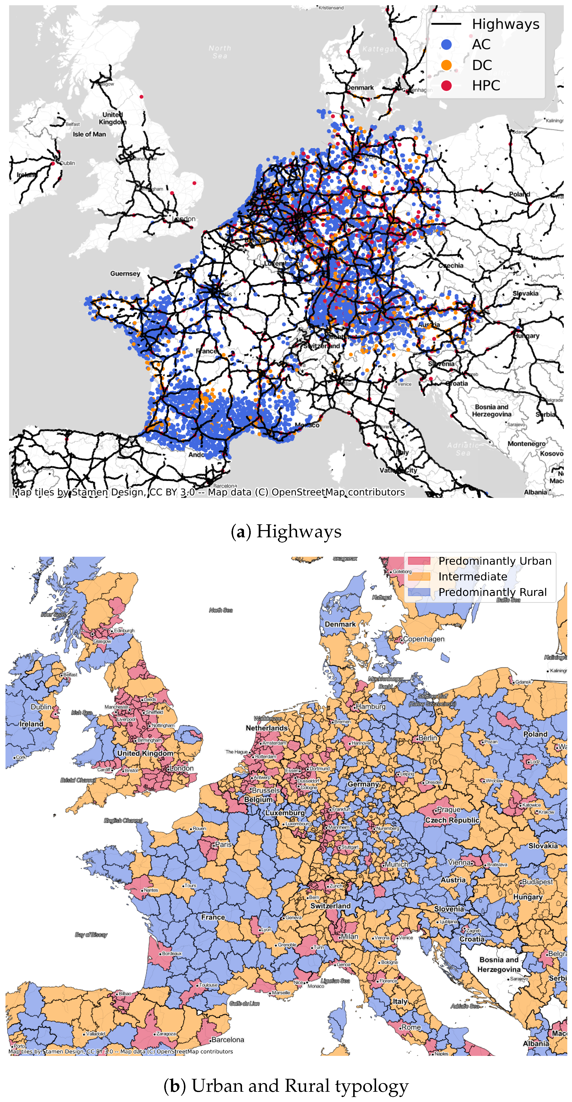
Figure A3.
European highways and urban and rural typology.
Figure A3.
European highways and urban and rural typology.
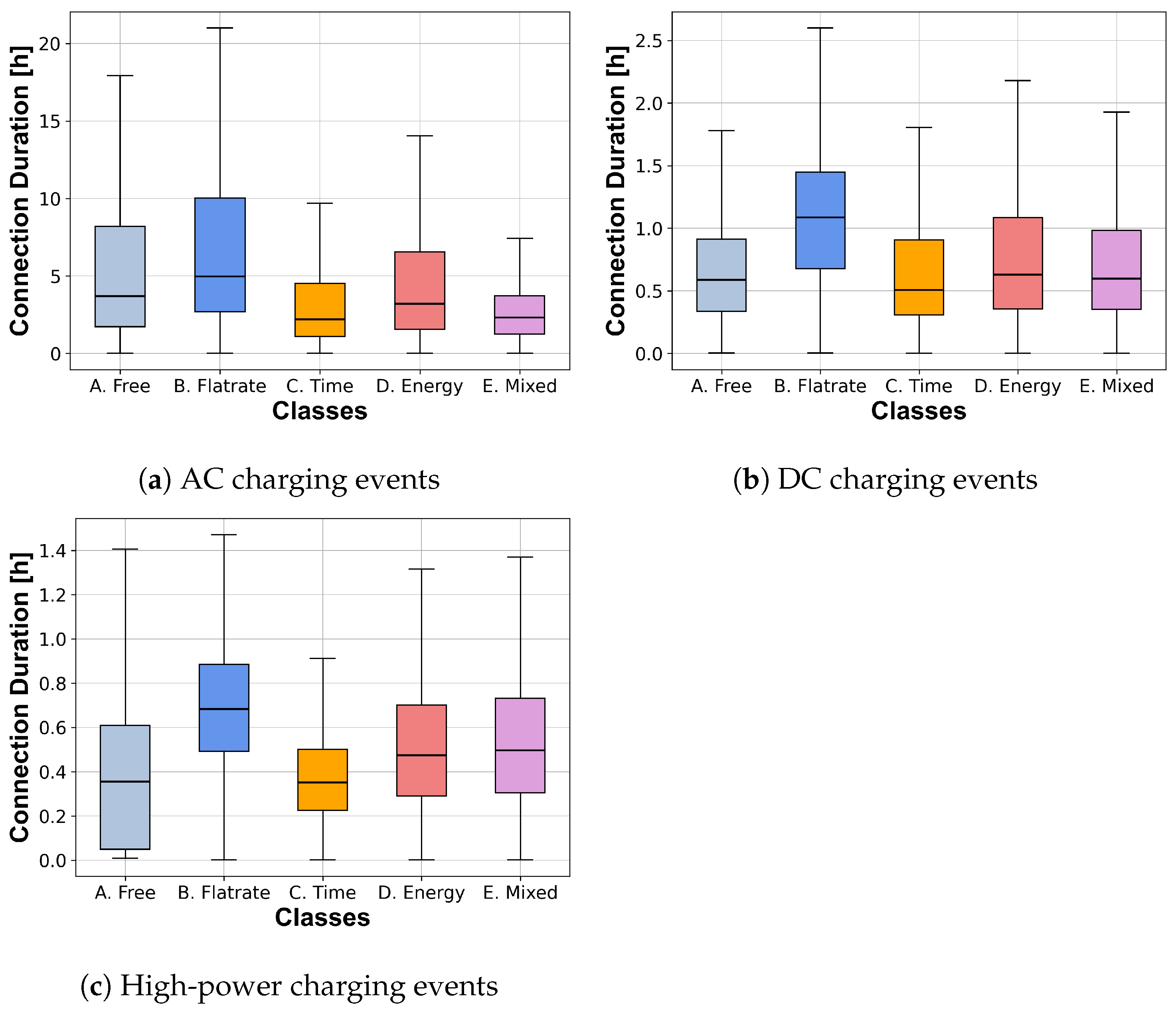
Figure A4.
Connection duration of AC, DC, and high-power charging events.
Figure A4.
Connection duration of AC, DC, and high-power charging events.
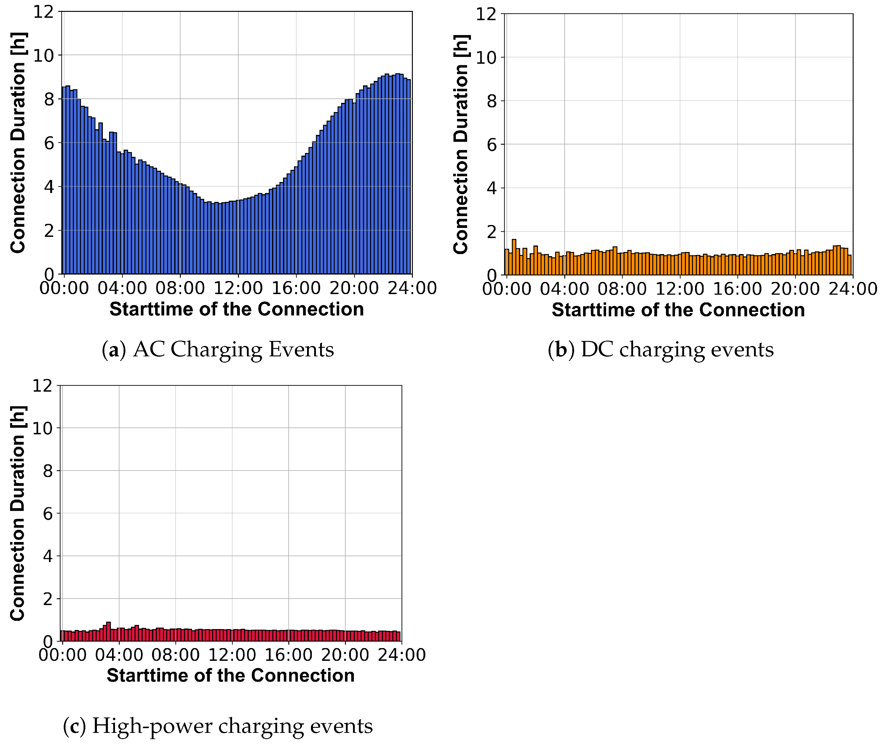
Figure A5.
Average connection duration of AC, DC, and high-power charging events depending on the connection start time.
Figure A5.
Average connection duration of AC, DC, and high-power charging events depending on the connection start time.
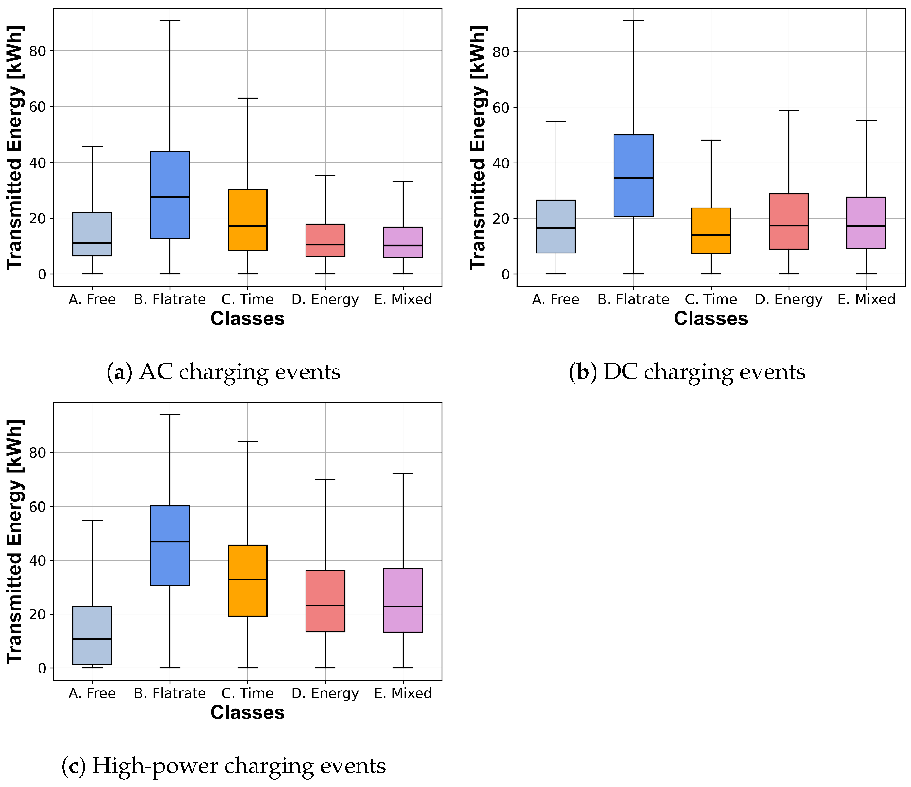
Figure A6.
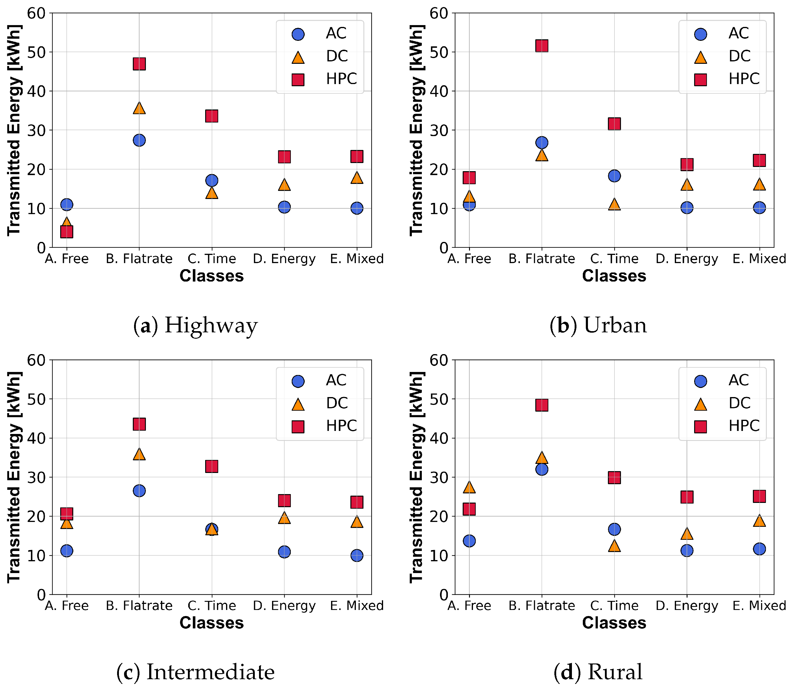
Transmitted energy of AC, DC and high-power charging events.
Figure A6.
Transmitted energy of AC, DC and high-power charging events.
Figure A7.
Connection duration for location type highway per pricing model class of AC, DC, and high-power charging events.
Figure A7.
Connection duration for location type highway per pricing model class of AC, DC, and high-power charging events.
Figure A8.
Connection duration for location type urban per pricing model class of AC, DC, and high-power charging events.
Figure A8.
Connection duration for location type urban per pricing model class of AC, DC, and high-power charging events.
Figure A9.
Connection duration for location type intermediate per pricing model class of AC, DC, and high-power charging events.
Figure A9.
Connection duration for location type intermediate per pricing model class of AC, DC, and high-power charging events.
Figure A10.
Connection duration for location type rural per pricing model class of AC, DC, and high power charging events.
Figure A10.
Connection duration for location type rural per pricing model class of AC, DC, and high power charging events.
Figure A11.
Transmitted energy for location type highway per pricing model class of AC, DC, and high-power charging events.
Figure A11.
Transmitted energy for location type highway per pricing model class of AC, DC, and high-power charging events.
Figure A12.
Transmitted energy for location type urban per pricing model class of AC, DC, and high-power charging events.
Figure A12.
Transmitted energy for location type urban per pricing model class of AC, DC, and high-power charging events.
Figure A13.
Transmitted energy for location type intermediate per pricing model class of AC, DC, and high-power charging events.
Figure A13.
Transmitted energy for location type intermediate per pricing model class of AC, DC, and high-power charging events.
Figure A14.
Transmitted energy for location type rural per pricing model class of AC, DC, and high-power charging events.
Figure A14.
Transmitted energy for location type rural per pricing model class of AC, DC, and high-power charging events.
Table A6.
Nominal charging power for AC, DC and high-power charging events from the real-world dataset.
Table A6.
Nominal charging power for AC, DC and high-power charging events from the real-world dataset.
| Charging Technology | Percentil 25% [kW] | Percentil 50% [kW] | Percentil 75% [kW] | Percentil 90% [kW] | Percentil 95% [kW] |
|---|
| AC | 22 | 22 | 22 | 22 | 22 |
| DC | 50 | 50 | 50 | 53 | 75 |
| HPC | 150 | 300 | 300 | 350 | 350 |
Table A7.
Average charging power for AC, DC, and high-power charging events from the real-world dataset.
Table A7.
Average charging power for AC, DC, and high-power charging events from the real-world dataset.
| Charging Technology | Percentil 25% [kW] | Percentil 50% [kW] | Percentil 75% [kW] | Percentil 90% [kW] | Percentil 95% [kW] |
|---|
| AC | 2.1 | 3.6 | 7.3 | 11.0 | 15.0 |
| DC | 19.8 | 31.2 | 42.2 | 48.2 | 61.3 |
| HPC | 36.0 | 54.6 | 81.1 | 110.3 | 126.0 |
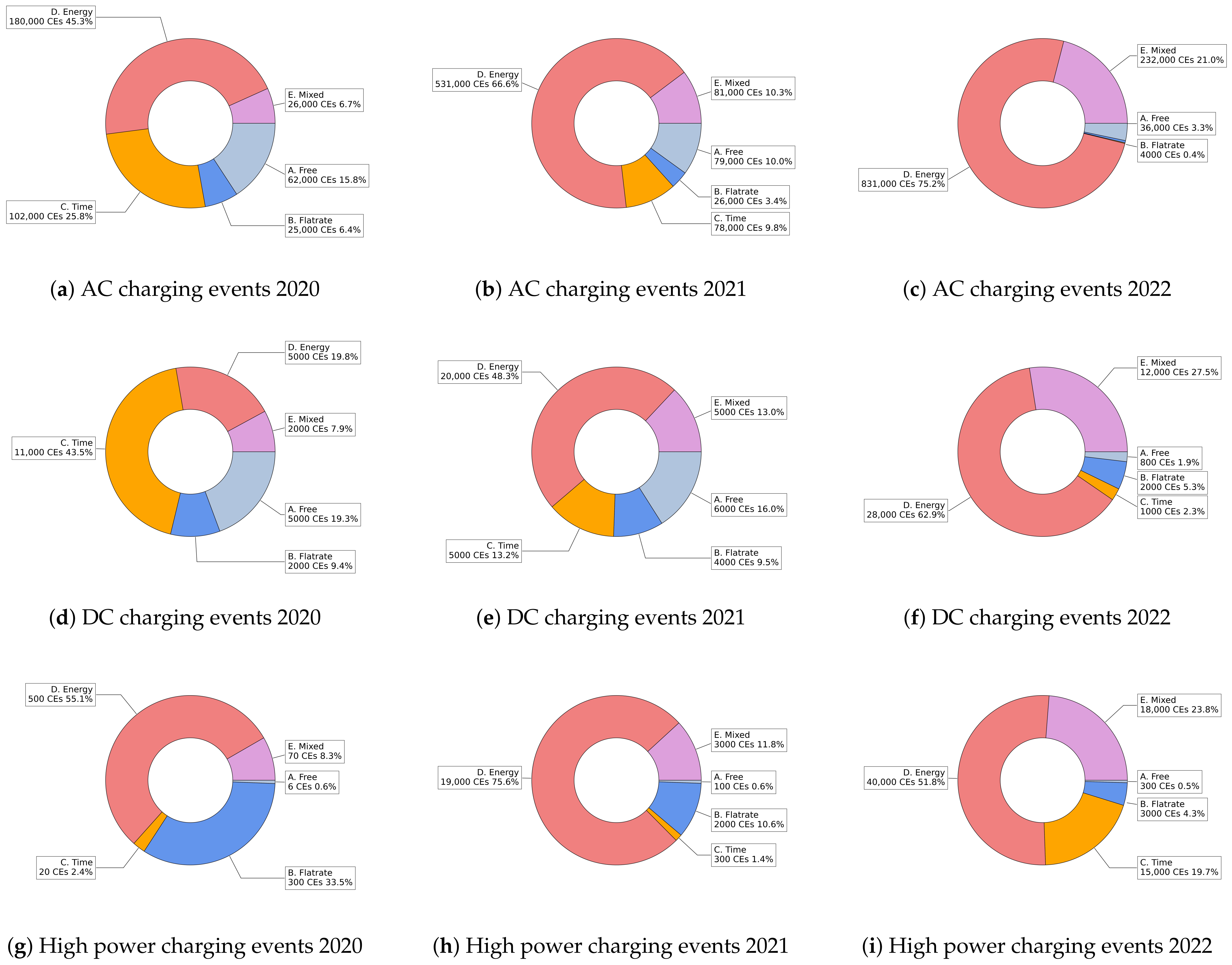
Figure A15.
Distribution of the classified pricing models per country and period of time in the dataset.
Figure A15.
Distribution of the classified pricing models per country and period of time in the dataset.
Table A8.
Connection duration per pricing model class for AC, DC, and high-power charging events.
Table A8.
Connection duration per pricing model class for AC, DC, and high-power charging events.
| Charging Technology | Class | Percentil 25% [h] | Percentil 50% [h] | Percentil 75% [h] | Percentil 90% [h] | Percentil 95% [h] |
|---|
| AC | A. Free | 1.70 | 3.63 | 8.09 | 13.55 | 17.13 |
| AC | B. Flatrate | 2.70 | 4.90 | 9.92 | 14.80 | 17.93 |
| AC | C. Time | 1.10 | 2.20 | 4.47 | 10.52 | 12.48 |
| AC | D. Energy | 1.58 | 3.25 | 6.77 | 13.26 | 16.12 |
| AC | E. Mixed | 1.26 | 2.35 | 3.75 | 7.55 | 11.72 |
| DC | A. Free | 0.33 | 0.58 | 0.91 | 1.25 | 1.51 |
| DC | B. Flatrate | 0.71 | 1.09 | 1.45 | 1.82 | 2.50 |
| DC | C. Time | 0.30 | 0.50 | 0.89 | 1.44 | 1.98 |
| DC | D. Energy | 0.36 | 0.64 | 1.08 | 1.68 | 2.37 |
| DC | E. Mixed | 0.36 | 0.60 | 1.01 | 1.48 | 1.82 |
| HPC | A. Free | 0.04 | 0.34 | 0.60 | 0.83 | 1.03 |
| HPC | B. Flatrate | 0.50 | 0.69 | 0.88 | 1.09 | 1.27 |
| HPC | C. Time | 0.25 | 0.36 | 0.51 | 0.65 | 0.76 |
| HPC | D. Energy | 0.29 | 0.47 | 0.69 | 0.96 | 1.16 |
| HPC | E. Mixed | 0.31 | 0.49 | 0.73 | 0.98 | 1.15 |
Table A9.
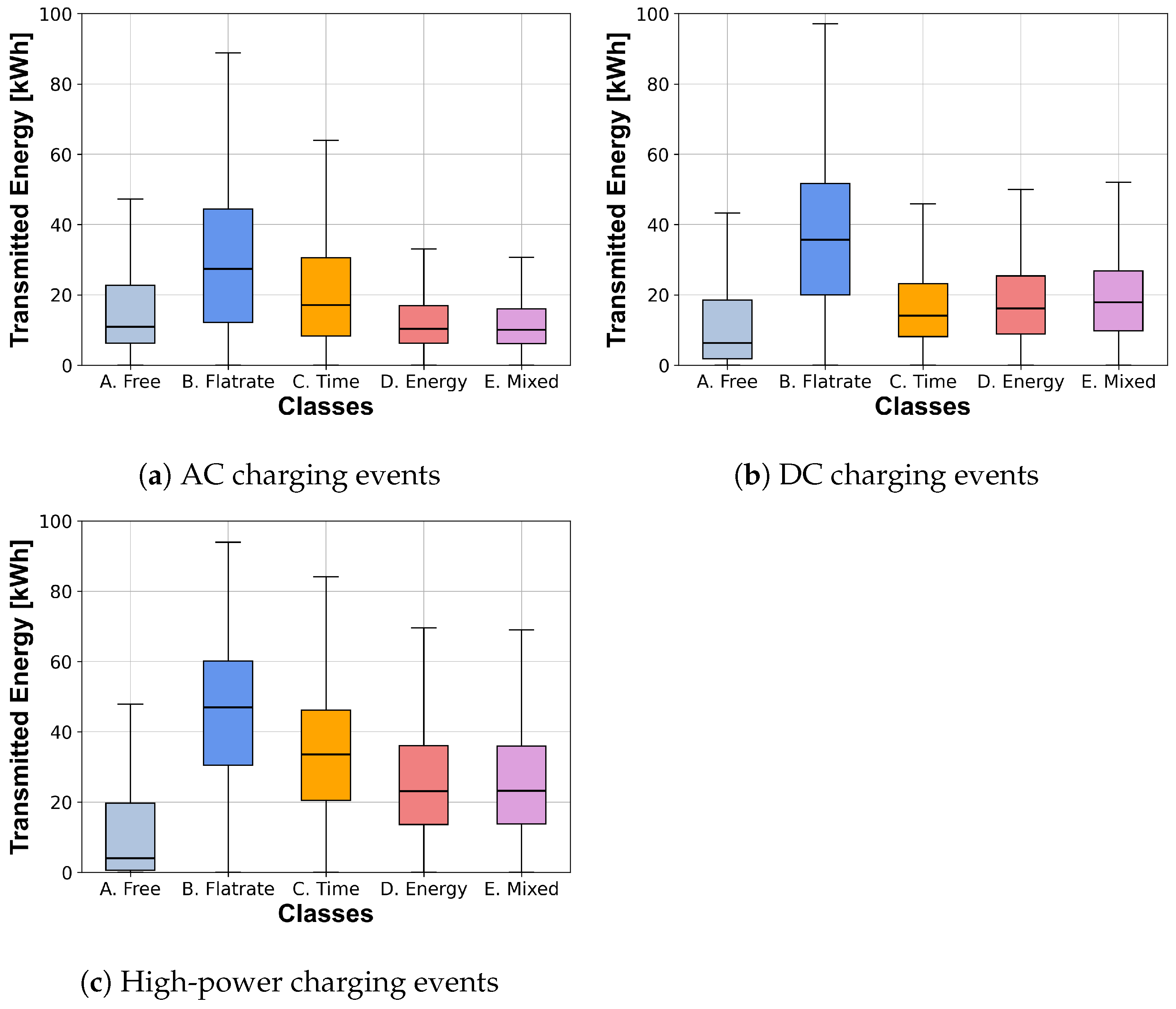
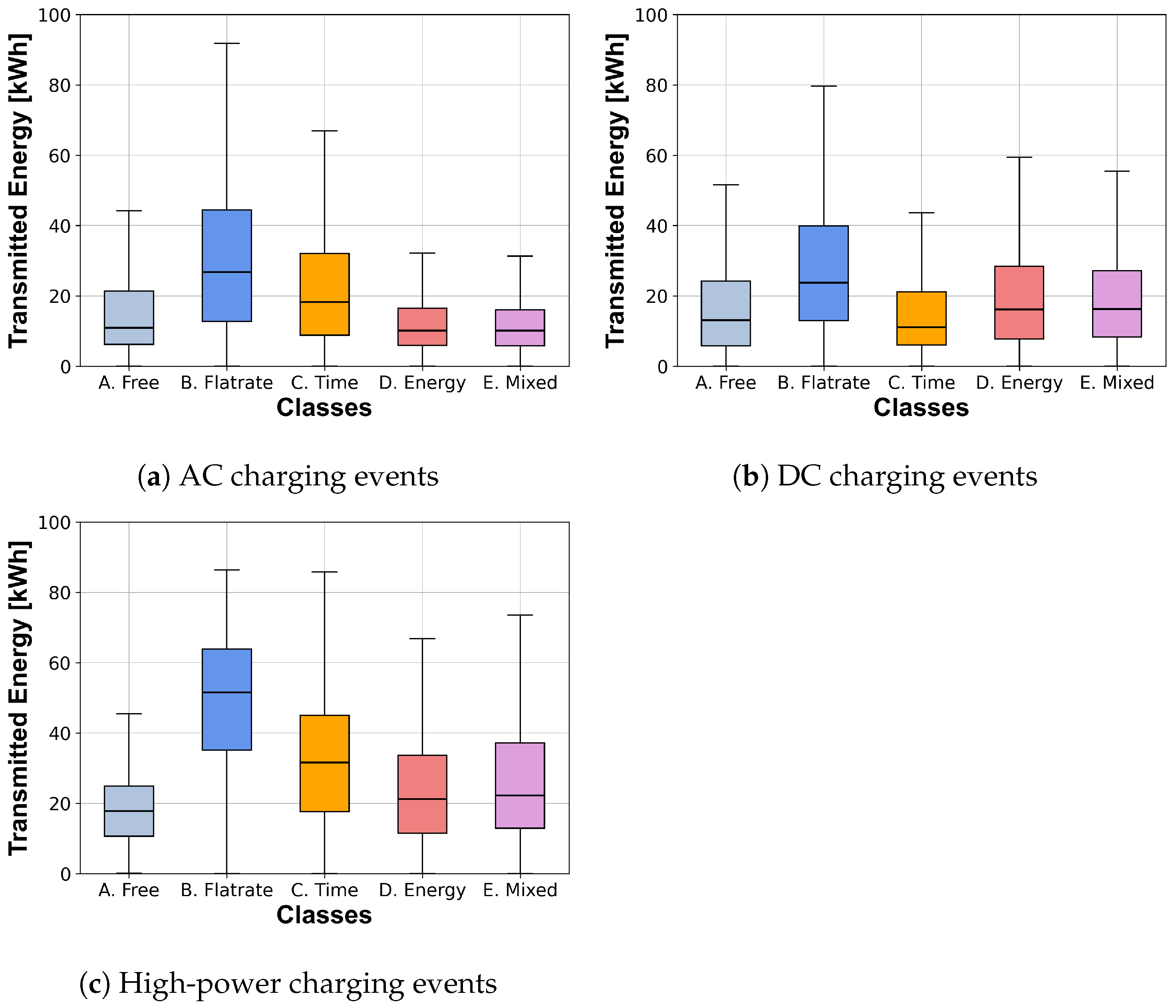
Transmitted energy per class for AC, DC, and high-power charging events.
Table A9.
Transmitted energy per class for AC, DC, and high-power charging events.
| Charging Technology | Class | Percentil 25% [kWh] | Percentil 50% [kWh] | Percentil 75% [kWh] | Percentil 90% [kWh] | Percentil 95% [kWh] |
|---|
| AC | A. Free | 6.38 | 11.04 | 21.96 | 36.83 | 46.67 |
| AC | B. Flatrate | 12.75 | 27.70 | 44.31 | 59.54 | 66.72 |
| AC | C. Time | 8.59 | 17.37 | 30.35 | 41.93 | 49.62 |
| AC | D. Energy | 6.24 | 10.42 | 17.95 | 33.41 | 42.20 |
| AC | E. Mixed | 5.9 | 10.26 | 16.84 | 31.36 | 39.88 |
| DC | A. Free | 7.56 | 16.39 | 26.42 | 39.66 | 48.96 |
| DC | B. Flatrate | 22.07 | 35.78 | 51.11 | 62.96 | 68.77 |
| DC | C. Time | 7.45 | 13.86 | 23.97 | 36.36 | 45.50 |
| DC | D. Energy | 9.26 | 17.69 | 29.02 | 42.64 | 51.49 |
| DC | E. Mixed | 9.38 | 17.60 | 28.05 | 39.76 | 47.95 |
| HPC | A. Free | 1.16 | 10.71 | 22.65 | 37.90 | 49.12 |
| HPC | B. Flatrate | 31.82 | 47.74 | 60.72 | 69.40 | 73.88 |
| HPC | C. Time | 21.40 | 34.26 | 46.50 | 55.55 | 60.34 |
| HPC | D. Energy | 13.77 | 23.38 | 36.21 | 49.26 | 56.92 |
| HPC | E. Mixed | 13.27 | 22.68 | 30.54 | 50.43 | 57.67 |
Table A10.
Average charging power per class for AC, DC, and high-power charging events.
Table A10.
Average charging power per class for AC, DC, and high-power charging events.
| Charging Technology | Class | Percentil 25% [kW] | Percentil 50% [kW] | Percentil 75% [kW] | Percentil 90% [kW] | Percentil 95% [kW] |
|---|
| AC | A. Free | 1.74 | 3.42 | 6.90 | 10.59 | 12.55 |
| AC | B. Flatrate | 3.00 | 5.39 | 9.48 | 11.19 | 15.14 |
| AC | C. Time | 3.35 | 7.09 | 12.89 | 17.65 | 19.98 |
| AC | D. Energy | 1.86 | 3.46 | 6.96 | 10.72 | 11.96 |
| AC | E. Mixed | 2.81 | 3.92 | 8.33 | 11.13 | 15.74 |
| DC | A. Free | 20.22 | 29.53 | 38.94 | 45.91 | 47.65 |
| DC | B. Flatrate | 26.59 | 36.33 | 44.37 | 46.83 | 48.97 |
| DC | C. Time | 19.25 | 28.53 | 34.90 | 40.52 | 43.50 |
| DC | D. Energy | 18.13 | 29.63 | 41.21 | 46.27 | 48.65 |
| DC | E. Mixed | 19.00 | 29.76 | 41.30 | 46.23 | 48.53 |
| HPC | A. Free | 19.90 | 32.34 | 52.78 | 79.60 | 87.89 |
| HPC | B. Flatrate | 48.83 | 68.23 | 88.62 | 112.88 | 125.79 |
| HPC | C. Time | 66.95 | 93.10 | 115.02 | 133.12 | 142.67 |
| HPC | D. Energy | 34.47 | 49.60 | 71.20 | 98.54 | 116.74 |
| HPC | E. Mixed | 30.58 | 45.70 | 69.02 | 94.57 | 110.13 |
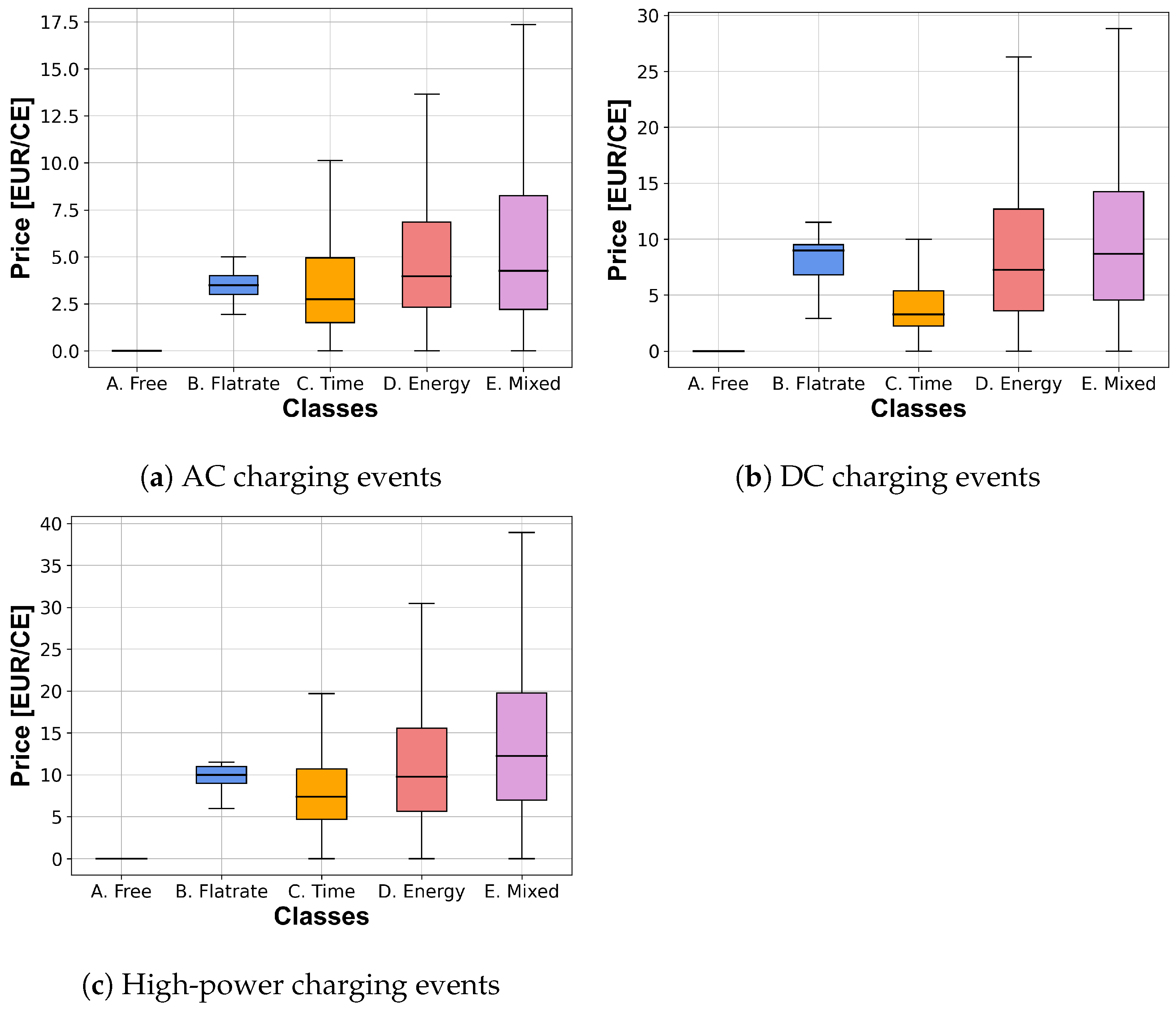
Table A11.
Price per CE and per class for AC, DC, and HPC CEs.
Table A11.
Price per CE and per class for AC, DC, and HPC CEs.
| Charging Technology | Class | Percentil 25% [Euro/CE] | Percentil 50% [Euro/CE] | Percentil 75% [Euro/CE] | Percentil 90% [Euro/CE] | Percentil 95% [Euro/CE] |
|---|
| AC | A. Free | 0 | 0 | 0 | 0 | 0 |
| AC | B. Flatrate | 3.00 | 3.50 | 4.38 | 6.00 | 6.82 |
| AC | C. Time | 1.50 | 2.73 | 4.95 | 8.43 | 11.94 |
| AC | D. Energy | 2.34 | 3.98 | 6.88 | 12.97 | 16.91 |
| AC | E. Mixed | 2.24 | 4.28 | 8.31 | 15.34 | 20.80 |
| DC | A. Free | 0 | 0 | 0 | 0 | 0 |
| DC | B. Flatrate | 7.00 | 9.00 | 9.50 | 11.00 | 11.50 |
| DC | C. Time | 2.27 | 3.27 | 5.21 | 8.30 | 11.31 |
| DC | D. Energy | 3.76 | 7.37 | 12.74 | 19.70 | 24.53 |
| DC | E. Mixed | 4.54 | 8.68 | 14.26 | 21.02 | 26.01 |
| HPC | A. Free | 0 | 0 | 0 | 0 | 0 |
| HPC | B. Flatrate | 9.00 | 9.99 | 11.00 | 15.00 | 15.00 |
| HPC | C. Time | 5.22 | 7.80 | 10.92 | 14.04 | 16.77 |
| HPC | D. Energy | 5.70 | 9.84 | 15.62 | 22.15 | 26.98 |
| HPC | E. Mixed | 6.99 | 12.27 | 19.77 | 28.00 | 33.24 |
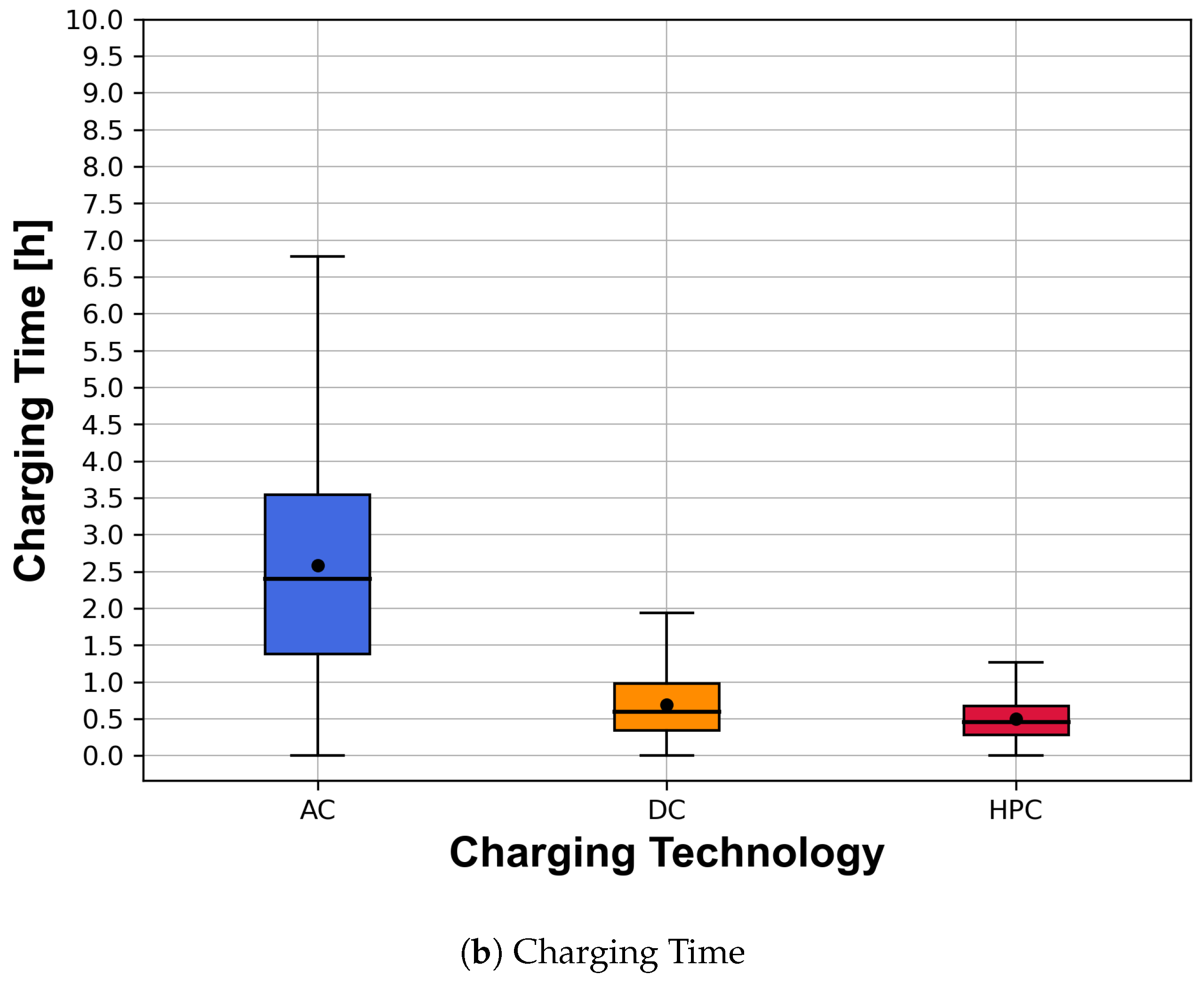
Table A12.
Charging time per charging event and per class for AC, DC, and high-power charging events.
Table A12.
Charging time per charging event and per class for AC, DC, and high-power charging events.
| Charging Technology | Class | Percentil 25% [h/CE] | Percentil 50% [h/CE] | Percentil 75% [h/CE] | Percentil 90% [h/CE] | Percentil 95% [h/CE] |
|---|
| AC | A. Free | 1.50 | 2.53 | 3.81 | 5.10 | 5.85 |
| AC | B. Flatrate | 2.45 | 3.91 | 5.31 | 6.48 | 7.23 |
| AC | C. Time | 1.08 | 2.09 | 3.61 | 5.10 | 5.87 |
| AC | D. Energy | 1.46 | 2.44 | 3.52 | 4.71 | 5.49 |
| AC | E. Mixed | 1.23 | 2.16 | 3.18 | 4.14 | 4.89 |
| DC | A. Free | 0.33 | 0.59 | 0.90 | 1.22 | 1.41 |
| DC | B. Flatrate | 0.70 | 1.06 | 1.38 | 1.56 | 1.79 |
| DC | C. Time | 0.30 | 0.50 | 0.85 | 1.28 | 1.50 |
| DC | D. Energy | 0.36 | 0.63 | 1.02 | 1.36 | 1.58 |
| DC | E. Mixed | 0.36 | 0.60 | 0.99 | 1.37 | 1.59 |
| HPC | A. Free | 0.04 | 0.34 | 0.60 | 0.78 | 0.92 |
| HPC | B. Flatrate | 0.50 | 0.68 | 0.88 | 1.08 | 1.21 |
| HPC | C. Time | 0.25 | 0.36 | 0.51 | 0.65 | 0.76 |
| HPC | D. Energy | 0.29 | 0.47 | 0.68 | 0.91 | 1.07 |
| HPC | E. Mixed | 0.31 | 0.49 | 0.72 | 0.96 | 1.11 |
Table A13.
Idle time per charging event and per class for AC, DC, and high-power charging events.
Table A13.
Idle time per charging event and per class for AC, DC, and high-power charging events.
| Charging Technology | Class | Percentil 25% [h/CE] | Percentil 50% [h/CE] | Percentil 75% [h/CE] | Percentil 90% [h/CE] | Percentil 95% [h/CE] |
|---|
| AC | A. Free | 0.20 | 1.09 | 4.29 | 8.45 | 11.27 |
| AC | B. Flatrate | 0.26 | 0.99 | 4.61 | 8.33 | 10.70 |
| AC | C. Time | 0.01 | 0.11 | 0.86 | 5.42 | 6.61 |
| AC | D. Energy | 0.12 | 0.81 | 3.25 | 8.55 | 10.64 |
| AC | E. Mixed | 0.03 | 0.19 | 0.57 | 3.40 | 6.83 |
| DC | A. Free | 0 | 0 | 0.01 | 0.04 | 0.10 |
| DC | B. Flatrate | 0 | 0.03 | 0.07 | 0.26 | 0.72 |
| DC | C. Time | 0 | 0 | 0.03 | 0.16 | 0.48 |
| DC | D. Energy | 0 | 0.01 | 0.06 | 0.32 | 0.79 |
| DC | E. Mixed | 0 | 0 | 0.02 | 0.12 | 0.23 |
| HPC | A. Free | 0 | 0 | 0.01 | 0.06 | 0.11 |
| HPC | B. Flatrate | 0 | 0 | 0.01 | 0.02 | 0.05 |
| HPC | C. Time | 0 | 0 | 0 | 0 | 0 |
| HPC | D. Energy | 0 | 0 | 0.01 | 0.05 | 0.09 |
| HPC | E. Mixed | 0 | 0 | 0 | 0.02 | 0.05 |
Table A14.
Correlation analysis per class for AC, DC, and high-power charging events.
Table A14.
Correlation analysis per class for AC, DC, and high-power charging events.
| Var. 1 | Var. 2 | AC Correlation | AC p-Value | DC Correlation | DC p-Value | HPC Correlation | HPC p-Value |
|---|
| A. Free | Duration | 0.0451 | 0 | −0.0505 | 1.4 | −0.0148 | 1.4 |
| B. Flatrate | Duration | 0.0588 | 0 | 0.0595 | 2.3 | 0.1044 | 8.0 |
| C. Time | Duration | −0.0546 | 0 | 0.0053 | 7.0 | −0.1229 | 0 |
| D. Energy | Duration | 0.0774 | 0 | 0.0288 | 1.5 | 0.0204 | 3.7 |
| E. Mixed | Duration | −0.1207 | 0 | −0.0432 | 1.5 | 0.0237 | 1.5 |
| A. Free | Energy | 0.0153 | 1.3 | −0.0443 | 5.5 | −0.0536 | 1.6 |
| B. Flatrate | Energy | 0.1715 | 0 | 0.2735 | 0 | 0.2555 | 0 |
| C. Time | Energy | 0.1096 | 0 | −0.1025 | 3.5 | 0.1003 | 1.9 |
| D. Energy | Energy | −0.0922 | 0 | −0.0258 | 2.2 | −0.1403 | 0 |
| E. Mixed | Energy | −0.0479 | 0 | −0.0242 | 2.0 | −0.0595 | 8.5 |
| A. Free | Avg. Power | −0.0334 | 0 | −0.0042 | 1.5 | −0.0474 | 3.1 |
| B. Flatrate | Avg. Power | 0.0359 | 0 | 0.0984 | 3.0 | 0.0683 | 8.9 |
| C. Time | Avg. Power | 0.2095 | 0 | −0.0711 | 2.1 | 0.3619 | 0 |
| D. Energy | Avg. Power | −0.1550 | 0 | −0.0151 | 3.0 | −0.1824 | 0 |
| E. Mixed | Avg. Power | 0.0554 | 0 | 0.0219 | 1.0 | −0.1280 | 0 |
| A. Free | Charge Time | 0.0314 | 0 | −0.0530 | 4.0 | −0.0343 | 9.7 |
| B. Flatrate | Charge Time | 0.1299 | 0 | 0.1896 | 0 | 0.1628 | 0 |
| C. Time | Charge Time | −0.0145 | 1.2 | −0.0814 | 1.1 | −0.1816 | 0 |
| D. Energy | Charge Time | −0.0009 | 1.6 | −0.0020 | 4.8 | 0.0110 | 3.3 |
| E. Mixed | Charge Time | −0.0682 | 0 | −0.0093 | 1.5 | 0.0554 | 4.0 |
| A. Free | Idle Time | 0.0396 | 0 | −0.0389 | 1.0 | 0.0098 | 1.4 |
| B. Flatrate | Idle Time | 0.0218 | 5.9 | 0.0097 | 1.0 | −0.0003 | 9.0 |
| C. Time | Idle Time | −0.0558 | 0 | 0.0289 | 1.2 | −0.0084 | 6.1 |
| D. Energy | Idle Time | 0.0864 | 0 | 0.0315 | 1.5 | 0.0182 | 3.6 |
| E. Mixed | Idle Time | −0.1114 | 0 | −0.0436 | 2.1 | −0.0163 | 1.2 |
Table A15.
Mann–Whitney-U analysis per class for AC charging events.
Table A15.
Mann–Whitney-U analysis per class for AC charging events.
| Class 1 | Class 2 | Duration s-Value | Duration p-Value | Energy s-Value | Energy p-Value |
|---|
| A. Free | B. Flatrate | 5.10 | 0 | 3.40 | 0 |
| A. Free | C. Time | 2.16 | 0 | 1.43 | 0 |
| A. Free | D. Energy | 1.67 | 0 | 1.66 | 0 |
| A. Free | E. Mixed | 4.52 | 0 | 3.88 | 0 |
| B. Flatrate | A. Free | 7.24 | 0 | 8.94 | 0 |
| B. Flatrate | C. Time | 8.27 | 0 | 7.58 | 0 |
| B. Flatrate | D. Energy | 6.52 | 0 | 7.89 | 0 |
| B. Flatrate | E. Mixed | 1.74 | 0 | 1.82 | 0 |
| C. Time | A. Free | 1.36 | 0 | 2.09 | 0 |
| C. Time | B. Flatrate | 3.51 | 0 | 4.20 | 0 |
| C. Time | D. Energy | 1.24 | 0 | 1.87 | 0 |
| C. Time | E. Mixed | 3.42 | 9.07 | 4.34 | 0 |
| D. Energy | A. Free | 1.46 | 0 | 1.46 | 0 |
| D. Energy | B. Flatrate | 3.95 | 0 | 2.58 | 0 |
| D. Energy | C. Time | 1.74 | 0 | 1.11 | 0 |
| D. Energy | E. Mixed | 3.62 | 0 | 3.09 | 5.81 |
| E. Mixed | A. Free | 2.60 | 0 | 3.24 | 0 |
| E. Mixed | B. Flatrate | 6.38 | 0 | 5.58 | 0 |
| E. Mixed | C. Time | 3.36 | 9.07 | 2.44 | 0 |
| E. Mixed | D. Energy | 2.41 | 0 | 2.94 | 5.81 |
Table A16.
Mann–Whitney-U analysis per class for DC charging events.
Table A16.
Mann–Whitney-U analysis per class for DC charging events.
| Class 1 | Class 2 | Duration s-Value | Duration p-Value | Energy s-Value | Energy p-Value |
|---|
| A. Free | B. Flatrate | 3.60 | 0 | 3.38 | 0 |
| A. Free | C. Time | 1.20 | 7.90 | 1.24 | 9.58 |
| A. Free | D. Energy | 3.45 | 1.54 | 3.57 | 3.63 |
| A. Free | E. Mixed | 1.48 | 1.25 | 1.48 | 2.06 |
| B. Flatrate | A. Free | 9.69 | 0 | 9.91 | 0 |
| B. Flatrate | C. Time | 1.35 | 0 | 1.45 | 0 |
| B. Flatrate | D. Energy | 4.06 | 0 | 4.40 | 0 |
| B. Flatrate | E. Mixed | 1.76 | 0 | 1.85 | 0 |
| C. Time | A. Free | 1.13 | 7.90 | 1.09 | 9.58 |
| C. Time | B. Flatrate | 5.20 | 0 | 4.24 | 0 |
| C. Time | D. Energy | 4.73 | 2.04 | 4.66 | 1.05 |
| C. Time | E. Mixed | 2.02 | 8.30 | 1.93 | 3.94 |
| D. Energy | A. Free | 4.14 | 1.54 | 4.02 | 3.63 |
| D. Energy | B. Flatrate | 2.02 | 0 | 1.68 | 0 |
| D. Energy | C. Time | 5.94 | 2.04 | 6.01 | 1.05 |
| D. Energy | E. Mixed | 7.46 | 6.57 | 7.24 | 1.05 |
| E. Mixed | A. Free | 1.64 | 1.25 | 1.64 | 2.06 |
| E. Mixed | B. Flatrate | 7.49 | 0 | 6.61 | 0 |
| E. Mixed | C. Time | 2.37 | 8.30 | 2.46 | 3.94 |
| E. Mixed | D. Energy | 6.85 | 6.57 | 7.07 | 1.05 |
Table A17.
Mann–Whitney-U analysis per class for high-power charging events.
Table A17.
Mann–Whitney-U analysis per class for high-power charging events.
| Class 1 | Class 2 | Duration s-Value | Duration p-Value | Energy s-Value | Energy p-Value |
|---|
| A. Free | B. Flatrate | 9.32 | 3.25 | 4.80 | 3.82 |
| A. Free | C. Time | 4.37 | 4.14 | 2.03 | 1.14 |
| A. Free | D. Energy | 1.37 | 3.31 | 1.09 | 2.07 |
| A. Free | E. Mixed | 4.71 | 4.83 | 3.87 | 4.09 |
| B. Flatrate | A. Free | 2.95 | 3.25 | 3.41 | 3.82 |
| B. Flatrate | C. Time | 9.09 | 0 | 7.70 | 0 |
| B. Flatrate | D. Energy | 3.03 | 0 | 3.51 | 0 |
| B. Flatrate | E. Mixed | 1.05 | 0 | 1.24 | 0 |
| C. Time | A. Free | 4.84 | 4.14 | 7.18 | 1.14 |
| C. Time | B. Flatrate | 2.12 | 0 | 3.51 | 0 |
| C. Time | D. Energy | 3.88 | 0 | 6.61 | 0 |
| C. Time | E. Mixed | 1.31 | 0 | 2.34 | 0 |
| D. Energy | A. Free | 2.35 | 3.31 | 2.64 | 2.07 |
| D. Energy | B. Flatrate | 1.50 | 0 | 1.02 | 0 |
| D. Energy | C. Time | 6.86 | 0 | 4.13 | 0 |
| D. Energy | E. Mixed | 7.46 | 8.19 | 7.70 | 0.53 |
| E. Mixed | A. Free | 8.55 | 4.83 | 9.38 | 4.09 |
| E. Mixed | B. Flatrate | 5.61 | 0 | 3.71 | 0 |
| E. Mixed | C. Time | 2.51 | 0 | 1.48 | 0 |
| E. Mixed | D. Energy | 7.99 | 8.19 | 7.75 | 0.53 |
Figure A16.
Charging and idle time of AC, DC and high-power charging events.
Figure A16.
Charging and idle time of AC, DC and high-power charging events.
Figure A17.
Average charging and idle time of AC, DC, and high-power charging events depending on the connection start time.
Figure A17.
Average charging and idle time of AC, DC, and high-power charging events depending on the connection start time.


