Article

A Lithium-Ion Battery Remaining Useful Life Prediction Model Based on CEEMDAN Data Preprocessing and HSSA-LSTM-TCN

1
Key Laboratory of Network and Communications, Dalian University, Dalian 116622, China
2
Beijing Jingwei Hirain Technology Company, Beijing 100020, China
3
ChengMai Technology (NanJing) Company, Beijing 100080, China
*
Author to whom correspondence should be addressed.
World Electr. Veh. J. 2024, 15(5), 177; https://doi.org/10.3390/wevj15050177
Submission received: 31 January 2024 / Revised: 10 April 2024 / Accepted: 11 April 2024 / Published: 24 April 2024
(This article belongs to the Special Issue Lithium-Ion Batteries for Electric Vehicle)

Abstract

:
Accurate prediction of the Remaining Useful Life (RUL) of lithium-ion batteries is crucial for reducing battery usage risks and ensuring the safe operation of systems. Addressing the impact of noise and capacity regeneration-induced nonlinear features on RUL prediction accuracy, this paper proposes a predictive model based on Complete Ensemble Empirical Mode Decomposition with Adaptive Noise (CEEMDAN) data preprocessing and IHSSA-LSTM-TCN. Firstly, CEEMDAN is used to decompose lithium-ion battery capacity data into high-frequency and low-frequency components. Subsequently, for the high-frequency component, a Temporal Convolutional Network (TCN) prediction model is employed. For the low-frequency component, an Improved Sparrow Search Algorithm (IHSSA) is utilized, which incorporates iterative chaotic mapping and a variable spiral coefficient to optimize the hyperparameters of Long Short-Term Memory (LSTM). The IHSSA-LSTM prediction model is obtained and used for prediction. Finally, the predicted values of the sub-models are combined to obtain the final RUL result. The proposed model is validated using the publicly available NASA dataset and CALCE dataset. The results demonstrate that this model outperforms other models, indicating good predictive performance and robustness.

1. Introduction

Lithium-ion batteries, known for their superior performance attributes such as fast charging rates and long operational lifespans, are widely utilized in the fields of new energy vehicles, communication devices, and aerospace electronic equipment [1,2,3]. However, as the number of charge–discharge cycles accumulates, the performance of lithium batteries inevitably degrades, and the Remaining Useful Life (RUL also decreases, ultimately leading to system malfunctions or even potential safety incidents [4,5]. Therefore, the efficient and accurate prediction of the RUL of lithium batteries holds significant practical importance [6,7]. The RUL of lithium-ion batteries [8] is defined as the remaining number of usable cycles from the prediction start point until the end of battery life. The battery life is considered to have ended when the actual capacity of the battery degrades to the failure threshold. The commonly used equation for RUL is as follows:
RUL = EOL N
In the equation, N represents the initial cycle position, and EOL denotes the cycle count at which the battery’s actual lifespan ends.
At present, there are primarily two approaches for predicting the RUL of lithium-ion batteries: model-based methods and data-driven methods [9,10].
The model-based methods approach to predicting the RUL of lithium-ion batteries involves analyzing internal physical and chemical reactions within the battery. This method requires constructing mathematical or physical models to describe the principles of performance degradation in lithium-ion batteries. For instance, equivalent circuit models and electrochemical models are established to accomplish RUL predictions for batteries [11,12,13]. Wang et al., with the assistance of Kalman Filtering (KF) and Particle Filtering (PF), studied battery predictions under different discharge rates and temperatures for RUL estimation [14]. Zhang et al. proposed an Unscented Particle Filtering (UPF) method for battery RUL prediction. The UPF was employed to forecast battery RUL, benefiting from the proposal distribution provided by the Unscented Kalman Filter (UKF) for particle sampling [15].
Model-based methods generally have complex structures and are susceptible to dynamic influences from external environmental factors. Additionally, they require a substantial amount of prior physical knowledge. The prediction accuracy of battery RUL is also dependent on the setting of model parameters. Establishing an accurate degradation prediction model can be challenging, and as a result, this approach has certain limitations [16].
In response to the limitations of the model-based approach, current research predominantly employs data-driven methods for predictive studies. These methods overcome the dependence on internal battery structures by investigating experimental data from the charging and discharging processes. Utilizing machine learning, deep learning, and various heuristic search algorithms, these approaches extract degradation features from capacity curves, significantly improving the accuracy of battery RUL predictions [17,18,19,20,21,22]. Kang et al. proposed a RUL prediction model based on fuzzy evaluation and Gaussian Process Regression (GPR). This method utilizes fuzzy evaluation, which combines expert knowledge and historical data to normalize observed data. The integration with the GPR model enables interval prediction of RUL, effectively expressing the uncertainty of prediction results [23]. Zhu et al. employed the Adaptive Boosting (AdaBoost) algorithm to mine data features and fused it with LSTM to construct a model for lithium-ion battery RUL prediction [24]. Liu et al. introduced a novel RUL prediction method using an Improved Sparrow Search Algorithm (ISSA) to optimize the LSTM network. By adjusting hyperparameters through ISSA, the prediction accuracy was enhanced [25]. While these studies exhibit high predictive accuracy, they are subject to the influence of data quality due to issues such as noise and capacity regeneration in some battery data [26].
Hence, Li et al. combined Empirical Mode Decomposition (EMD) with LSTM and Elman networks to predict capacity sequences at different frequencies [27]. However, traditional EMD suffers from mode-mixing issues. To address this, Tang introduced a hybrid RUL prediction model based on CEEMDAN and Gated Recurrent Unit (GRU) along with factor improvement using a genetic algorithm and dynamic population weighting to accelerate algorithm convergence [28]. Zhou et al. proposed a lithium-ion battery lifespan prediction model based on a TCN. Compared to traditional Recurrent Neural Network (RNN) models, this network structure has the capability to capture local regeneration phenomena [29].
In consideration of the strengths and limitations discussed in the literature, this paper introduces a lithium-ion battery RUL prediction method based on CEEMDAN data preprocessing and IHSSA-LSTM-TCN. Initially, the CEEMDAN is employed to decompose the lithium-ion battery capacity degradation sequence into high-frequency and low-frequency components. For the high-frequency component, a TCN model is utilized for prediction. For the low-frequency component, the IHSSA-LSTM model is proposed for prediction. Finally, the results from both components are integrated to obtain the ultimate prediction of lithium-ion battery RUL. The lithium-ion battery dataset provided by NASA and CALCE is selected for research purposes.

2. Introduction to Relevant Theories

2.1. CEEMDAN

The CEEMDAN is an improved version of the EEMD. The CEEMDAN decomposes nonlinear or non-stationary signals into a set of intrinsic mode functions, enhancing the signal-to-noise ratio and decomposition accuracy. Building upon the foundation of EEMD, the CEEMDAN incorporates adaptive noise handling. It addresses the issues of incomplete decomposition and significant reconstruction errors observed in EEMD, offering improved anti-pattern mixing performance [30,31]. The execution steps of the CEEMDAN are as follows:
(1)
Introduce Gaussian white noise ε 0 ω ( i ) ( t ) with an initial amplitude ε 0 to the original battery capacity sequence C ( t ) , forming a new capacity sequence, as shown in Equation (2). Here, t represents the number of cycles of the battery.
C i ( t ) = ε 0 ω ( i ) ( t ) + C ( t )
(2)
Using EMD to decompose C i ( t ) for i iterations, a series of intrinsic mode functions I M F s is obtained. Taking the overall average of these functions yields the first mode component I M F 1 of the battery decomposition, as shown in Equation (3).
I M F 1 = 1 I i = 1 I I M F 1 i
(3)
Calculate the first unique residual signal from the battery decomposition, obtaining Equation (4).
R 1 t = C t I M F 1
(4)
E k denotes the k-th mode component obtained after EMD processing. In each of the experiments, the signal R 1 ( t ) + ε 1 E 1 ( ω ( i ) ( t ) ) is decomposed, resulting in the second mode component and the second residual signal, as expressed in Equations (5) and (6).
I M F 2 = 1 I i = 1 I E 1 R 1 t + ε 1 E 1 ω i t
R 2 ( t ) = R 1 ( t ) I M F 2
(5)
For the k-th stage, repeat Step (4), continually decomposing the signal and calculating the (k + 1)-th mode component, as expressed in Equation (7).
I M F k + 1 = 1 I i = 1 I E 1 ( R k ( t ) + ε k E k ( ω ( i ) ( t ) ) )
(6)
Repeat Step (5) until the residual signal can no longer be further decomposed. At this point, the final number of mode components obtained is K. Decomposition stops, and the original signal is expressed as Equation (8).
C ( t ) = R ( t ) + k = 1 K I M F k

2.2. TCN

A TCN is a novel network architecture based on a Convolutional Neural Network (CNN), characterized by its incorporation of causal convolutions, dilated convolutions, and residual connections on the foundation of one-dimensional convolutional neural networks.
In causal convolutions, it is crucial to ensure that future time sequences do not leak information to the past, maintaining consistency in input and output sequence lengths. However, due to the unidirectional nature of causal convolutions, akin to RNN, processing long sequences necessitates numerous convolutional operations, leading to challenges such as excessive computational load and gradient vanishing. To address this issue, the TCN employs dilated convolutions.
To afford the sequence a larger receptive field, the TCN enhances causal convolutions by introducing a dilation factor, exponentially increasing the size of the receptive field. For a one-dimensional time sequence { x 1 , x 2 , , x t } and a filter { f 1 , f 2 , , f k } , the formula for dilated convolution at position x m is expressed in Equation (9).
F ( t ) = ( x × d f ) ( t ) = n = 0 k 1 f ( n ) × x t d × n
In the convolution operation, k represents the convolution kernel size; d is the dilation factor; t stands for the time sequence; and x t d × n indicates convolution operations applied exclusively to past data.
Dilated causal convolution can be divided into three parts: dilation, causality, and convolution. Convolution refers to a type of sliding operation performed by the convolution kernel on the data. Dilation refers to allowing interval sampling when convolving the input. Causality refers to the data at time t in the i-th layer, which only depends on the influence of the value at time t and before in the (i − 1)th layer. Figure 1 depicts the architectural diagram of the dilated causal convolution, with the k equal to 3 and the d set as [1, 2, 4].
Residual connections serve as an effective method for training deep neural networks, facilitating the transmission of information across layers and mitigating issues associated with gradient explosion and vanishing gradients in excessively deep networks.

2.3. LSTM

LSTM, a variant of a RNN, is distinguished by its incorporation of gates, namely the forget gate, memory gate, and output gate. These gates enable selective memorization or forgetting of specific portions of input data, preserving their historical states throughout computations. The fundamental architecture of LSTM is depicted in Figure 2, and the computational formulas for the propagation process are expressed in Equations (10)–(15).
f t = σ ( W f [ h t 1 , X t ] + b f )
i t = σ ( W i [ h t 1 , X t ] + b i )
C t ¯ = tan h ( W c [ h t 1 , X t ] + b c )
C t = f t C t 1 + i t C t ¯
O t = σ ( W o [ h t 1 , X t ] + b o )
h t = O t tan h ( C t )
In the above equations, X t and h t represent the input and hidden states at time t, respectively. f t , i t , and O t denote the states of the forget gate, input gate, and output gate, respectively. C t and C t 1 correspond to the current and previous time step’s cell states, while C ¯ t represents the candidate cell state. W f , W f , W c , W o , and b f , b i , b c , b o are matrices and bias values associated with the forget gate, input gate, cell state, and output gate, respectively. The symbol σ represents the Sigmoid activation function in the hidden layer.

2.4. SSA

A SSA is a metaheuristic optimization algorithm that mimics the predatory behavior of sparrows and their interactions with predators. The core concept involves dividing the search space into multiple subspaces, with each subspace explored individually until a target is found or the entire search space is covered [32].
In the SSA, each sparrow plays one of three distinct roles: discoverer, follower, or vigilante. The discoverer’s primary responsibility is to forage for food, while the follower closely tracks the discoverer, moving to the discoverer’s location to share in the food findings. The vigilante’s role is to safeguard the population and raise an alert when potential threats are detected.
In the context of predation, the discoverer exhibits two states. When no predators are detected nearby, the discoverer conducts an extensive, wide-area search. In the presence of predators, it relocates to a safer area, updating its location according to Equation (16):
X i , j t = X i , j t × exp i α × i i t e r m a x X i , j t + Q × L , R S T , R < S T
X i , j t denotes the position information of the i-th sparrow when dimension j is iterated t times; a is a random number uniformly distributed between (0, 1]; Q is a random number that follows a standard normal distribution; L represents a 1 × d matrix with all elements set to 1; R [ 0 , 1 ] is a uniformly distributed random number representing the warning value of the population; and S T [ 0.5 , 1 ] , is a pre-set normal number, representing the safe value of the population.
Throughout the foraging process, the follower continuously observes the discoverer. Upon the discoverer identifying high-quality food, the follower promptly relocates to the same area. The formula for updating the follower’s location is presented in Equation (17):
X i , j t + 1 = Q × exp X w o r s t t X i , j t i 2 , i > N 2 X p t + 1 + X i t X p t + 1 × A + × L , o t h e r w i s e
X P and X w o r s t represent the current optimal position and worst position, respectively. A + = A T ( A A T ) 1 , A denotes a 1 × m matrix, and the elements are randomly assigned to 1 or −1.
In the anti-predation phase, about 10% to 20% of the sparrows in the population are assigned as vigilantes. In the face of danger, an alarm mechanism is activated. The formula for updating the position of the vigilante is outlined in Equation (18):
X i . j t + 1 = X b e s t t + β × X i t X b e s t t , f i > f g X i t + K × ( X i t X w o r s t t ( f i f w ) + ε ) , f i = f g
X b e s t represents the optimal position; β is a random number following the standard normal distribution; f i is the current fitness of the sparrow; f g and f w are the current global optimal and worst values, respectively; K [−1, 1] is a uniformly distributed random number indicating the direction in which the sparrow moves; and ε is a normal number to avoid a fraction of 0.

3. CEEMDAN-IHSSA-LSTM-TCN Prediction Model

3.1. IHSSA

Compared to traditional intelligent algorithms, the SSA exhibits superior optimization performance. However, when directly applied to the nonlinear and complex task of battery RUL prediction, the SSA faces challenges during iterations, as it may be easily attracted to one of the optimal solutions, potentially overlooking other possible optima. This tendency to converge to a local optimum can hinder the algorithm’s ability to manifest global search capabilities during the optimization process, ultimately limiting its potential to enhance the prediction accuracy of lithium-ion battery RUL models [33,34]. To address this limitation, this paper introduces a multi-strategy improvement algorithm, the IHSSA, which incorporates certain enhancements to the SSA.
In the SSA, individual sparrow positions are initially generated through random initialization, which can result in an uneven distribution of sparrows in space. This non-uniform distribution may, in turn, reduce the algorithm’s solution accuracy and increase the search time. To mitigate the disruption caused by the inherent instability of the sparrow population, this paper employs iterative chaotic mapping, ultimately enhancing the algorithm’s accuracy in identifying high-quality locations.
Chaotic mapping is mathematical sequences characterized by high complexity and unpredictability. The sequences exhibit properties such as nonlinearity, sensitive dependence, and pseudo-randomness. Iterative chaotic mapping is a notable example of chaotic mapping, and its expression is delineated in Equation (19):
x k + 1 = sin ( a π x k )
x is the current iteration value and a (0, 1) is the control parameter. Iterative chaotic mapping was used to initialize the location and fitness value of the sparrow population, where a = 0.7 was set and the number of iterations was 200. The results are depicted in Figure 3.
In the SSA, when followers are in the majority, that is, (i > N/2), the global search capability is relatively weak. This situation is further exacerbated by the constraints of the search area’s boundaries, which can lead to clustering at the perimeter. Such clustering results in reduced population diversity and makes it challenging to escape local optima, thus hindering the algorithm’s search efficiency. To address this limitation, drawing inspiration from the spiral operation employed in the whale optimization algorithm, this paper introduces a variable spiral coefficient to the SSA. This addition allows for the control of the search step and direction, reducing the number of individuals congregating at the boundary. This, in turn, optimizes the utilization of the entire population space, circumvents the pitfalls of local extreme values, and ultimately enhances the global search performance of the SSA. The formula for the variable spiral coefficient is presented in Equation (20):
H = a × cos ( k × l × π ) , a = 1 , t < M 2 , e 5 l , otherwise , l = 1 2 × t M
H represents the variable spiral coefficient, where a is the parameter governing the spiral control, initially set at 1 and gradually diminishing in subsequent iterations. The parameter k denotes the spiral cycle, typically maintained at M/10, while l is a linearly decreasing parameter from 1 to −1 over the course of iterations. The variable t signifies the current iteration number, with M representing the maximum number of iterations.
Leveraging the insights derived from these considerations, coupled with Equations (17) and (20), the follower’s position is adjusted, and the update formula is refined to Equation (21):
X i , j t + 1 = cos ( a × l × π ) × exp ( X w o r s t t X i , j t i 2 ) , i > N 2   and   t < M 2 e 5 l × cos ( a × l × π ) × exp X w o r s t t X i , j t i 2 ,   i > N 2   and   t > M 2 X p t + 1 + X i t X p t + 1 × A + × L , otherwise

3.2. IHSSA-LSTM Prediction Model

The choice of hyperparameters for the LSTM model has a significant impact on the prediction accuracy of the model. Existing hyperparameter selection generally adopts empirical methods. Empirical methods are arbitrary and blind in parameter selection and lack universality. Their prediction effects are unstable and cannot achieve the best prediction effect. Therefore, by combining multiple hyperparameters into a multi-dimensional solution space, using Mean Square Error as the fitness function, and finding the information corresponding to the global optimal fitness value to obtain the optimal parameter combination, the randomness and blindness of the parameter selection can be reduced. The selection of multiple hyperparameters is often carried out at a larger solution speed, and a better performance optimization algorithm is needed to quickly obtain the global optimal solution. Therefore, the IHSSA with strong optimization ability and fast convergence speed is used to optimize the hyperparameters of the LSTM model to make up for the shortcomings of the LSTM model. By effectively obtaining the optimal parameter combination of prediction effects through intelligent algorithms, the scientific nature of model parameter selection is improved, thereby improving the predictive performance of the model. The specific steps of the IHSSA-LSTM model are as follows:
(1)
Divide the dataset into training and testing sets.
(2)
Initialize the parameters in the SSA, such as the number of individuals in the population N, the maximum number of iterations i_max, the proportion of discoverers in the population, the proportion of sentinels in the population, the safety threshold, etc.
(3)
Use chaotic iterative mapping to initialize the sparrow population.
(4)
Use the Mean Square Error as the fitness function, calculate the fitness value of the individual sparrows in the sparrow population, and obtain the optimal sparrow fitness value and their positions.
(5)
According to Equations (16), (18) and (21), update the positions of the producers, followers, and sentinels, respectively.
(6)
Select individuals based on the size of the fitness value and update the global optimal fitness value.
(7)
Repeat Step (4) until the termination condition is met. Output the position of the optimal sparrow individual, that is, the best hyperparameter value, input the obtained parameters into the LSTM model, and use the trained prediction model for prediction.
The primary steps of this model are as follows and the workflow is illustrated in Figure 4.

3.3. TCN Prediction Model

The TCN layer is composed of five convolutional modules, and each module consists of the dilated causal conv layer, the weight normalization layer, the PReLU layer, the dropout layer, and the residual connections. PreLU (Parametric Rectified Linear Unit), as an activation function, is a variant of ReLU (Rectified Linear Unit). It introduces a learnable parameter for negative input values, adaptively adjusting the shape of the activation function, thus enhancing the model’s flexibility and learning capacity in handling nonlinear issues. The definition of the PReLU activation function is as follows:
PReLU = x , x > 0 a x , x 0   and   0 < a < 1
Following these convolutional modules, a Squeeze-and-Excitation (SE) module is incorporated. The SE module dynamically adjusts the weights of different channel features based on the loss function, enhancing the network’s ability to recognize key information from the input sequence and determine its priority. This improves the overall efficiency of the TCN module. The summation operation ( ) ensures that the tensors remain consistent. The design of the TCN prediction model is illustrated in Figure 5.

3.4. CEEMDAN-IHSSA-LSTM-TCN Prediction Model Workflow

In summary, the proposed prediction model based on CEEMDAN data preprocessing and IHSSA-LSTM-TCN is designed to address challenges in lithium-ion batteries, such as capacity regeneration and noise interference. The goal is to enhance the predictive capability for the RUL of the batteries. After preprocessing the capacity data, the algorithm models and predicts using different models for the two components, followed by integrating the results to achieve the prediction of the RUL of lithium-ion batteries. This approach aims to enhance the accuracy of predicting the RUL of lithium-ion batteries. The complete workflow is illustrated in Figure 6, and the specific steps are outlined as follows:
(1)
Applying the CEEMDAN to preprocess the normalized lithium-ion battery capacity sequence, decomposition using sample entropy [35] results in three IMF components (high-frequency components) and one residual sequence R (low-frequency component).
(2)
Divide the data into training and testing sets.
(3)
Employing the TCN model for forecasting the IMFs components and utilizing the IHSSA-LSTM model for predicting the residual sequence R results in predictions for the two respective components.
(4)
Combining the predictions from the two components yields the final forecast for the RUL of lithium-ion batteries.

4. Experiments and Results Analysis

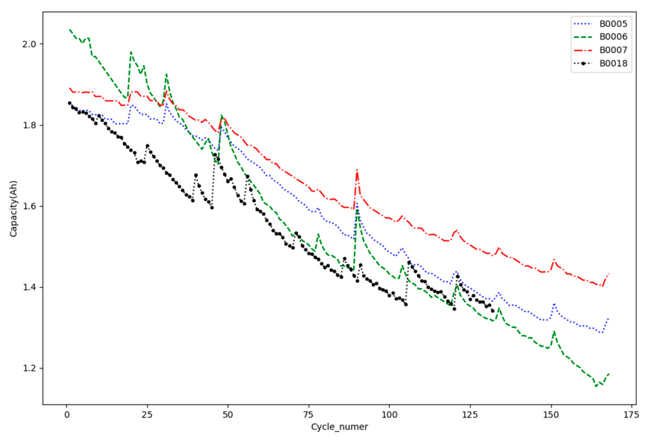
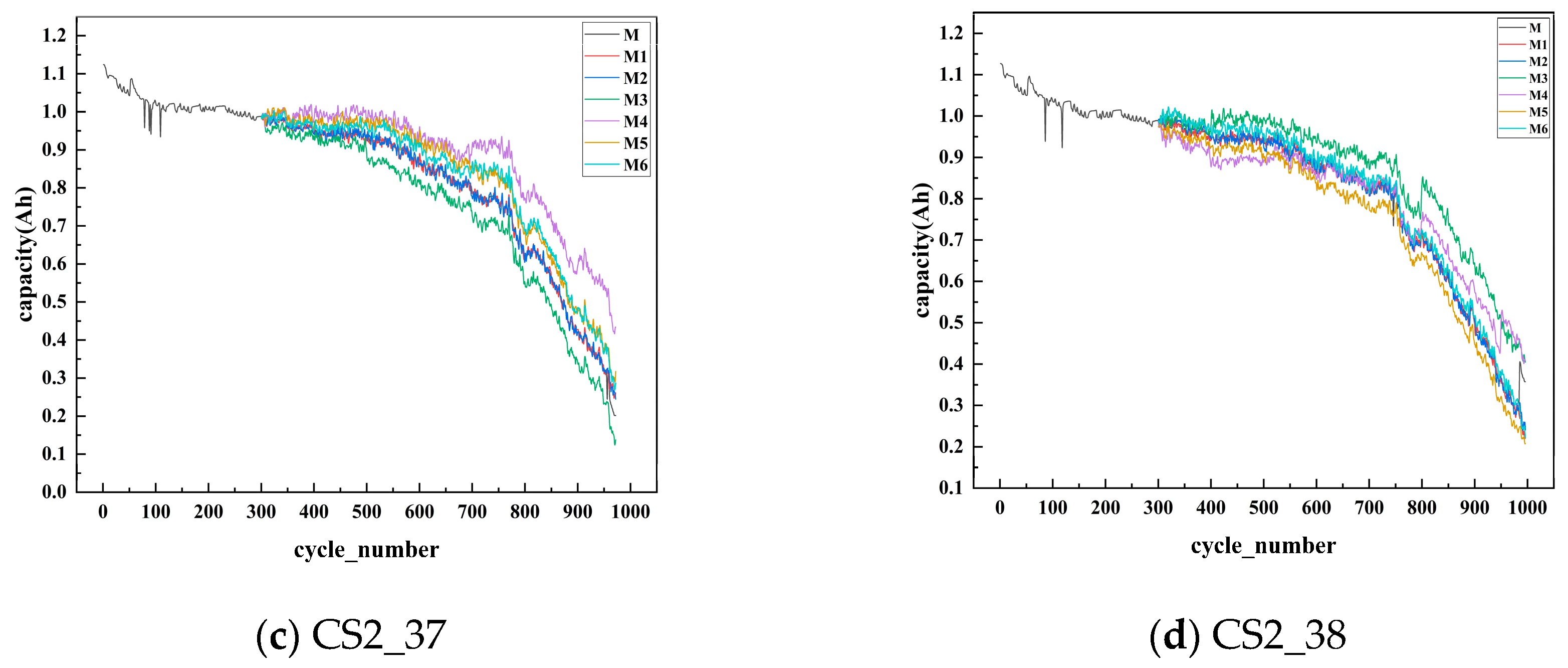
4.1. Introduction to the Experimental Dataset

To validate the accuracy of the proposed prediction method, lithium-ion battery datasets from the National Aeronautics and Space Administration (NASA) and the Center for Advanced Life Cycle Engineering (CALCE) at the University of Maryland were selected. The NASA battery dataset includes experiments on four types of lithium-ion batteries: B0005, B0006, B0007, and B0018. All batteries have a rated capacity of 2 Ah. The experiments were conducted at room temperature (24 °C). During the charging process, a standard charging method was used, with a constant current of 1.5 A until the maximum cut-off voltage of 4.2 V was reached. Then, it switched to constant voltage charging until the charging current dropped to 20 mA, indicating the end of the charging process. During discharge, the constant current was 2 A, and when the voltage reached the respective discharge cut-off voltages of 2.7 V, 2.5 V, 2.2 V, and 2.5 V for each of the four batteries, the discharge ended. The CALCE dataset includes CS2_35, CS2_36, CS2_37, and CS2_38. These batteries were also charged with a constant current rate of 0.5 °C until the battery voltage reached 4.2 V, followed by a constant voltage mode until the battery current dropped below 0.05 A. The discharge process was a constant current discharge of 0.05 A until the voltage dropped to 2.7 V. Figure 7 depicts the capacity decline curves of the four sets of batteries from NASA. Figure 8 depicts the capacity decline curves of the four sets of batteries from CALCE.
In battery experiments, it is generally accepted that the battery life is terminated when its current capacity reaches 70% of its rated capacity. Since the capacity of the B0007 battery did not drop below 1.4 Ah in the original dataset, for experimental rigor, the failure threshold for the B0007 battery was set at 1.5 Ah, while the other batteries were set at 1.4 Ah. In the dataset of CALCE, the failure threshold of the battery is 0.77 Ah.

4.2. Evaluation Metrics

To objectively measure the prediction model’s error, this study utilized Root Mean Square Error (RMSE) and Mean Absolute Error (MAE) as evaluation metrics for the prediction accuracy. They are defined as follows:
RMSE = 1 n t = 1 n ( x t x ^ t ) 2
MAE = 1 n t = 1 n x t x ^ t
In the above equations, x t is the predicted capacity value and x ^ t is the actual capacity value. RMSE represents the square root of the ratio of the squared deviations between the fitted data and the original data to the number of observations. MAE is the average distance between the predicted values of the model and the true values of the samples. Smaller values of RMSE and MAE indicate higher accuracy, better stability, and overall better model quality.

4.3. Process of the Experiment

As can be seen from Figure 7 and Figure 8, there are phenomena such as noise and capacity regeneration in the battery capacity. In order to reduce the interference of these phenomena on the data, CEEMDAN is used to decompose the capacity data. Taking the B0005 battery and CS2_35 battery as examples, they are decomposed into multiple groups of high-frequency signals and a group of residual signals, as shown in Figure 9.
It can be observed that, after decomposition, the high-frequency signal is able to retain the fluctuation information from the original signal. This is due to the capacity regeneration phenomenon that occurs during the charging and discharging process of the battery. Meanwhile, the residual signal constitutes a monotonically decreasing smooth sequence, indicating the primary degradation trend of the battery capacity.
We utilize sample entropy to evaluate the effect of decomposition. Sample entropy is an improved method based on approximate entropy to measure the complexity of a time series. It measures the complexity of a time series by measuring the probability of new changes in the signal. On the other hand, the calculation of sample entropy is independent of the length of the data, thus it has good consistency for the sequence before and after. The larger the sample entropy, the lower the stability and the higher the complexity of the time series. Figure 10 shows the sample entropy of the modes after decomposition for the B0005 battery and CS2_35 battery. As can be seen, the sample entropy of the modes has obvious differences and does not overlap, which indicates that the decomposition effect is good.
The high-frequency component is utilized as the input for the TCN prediction model, and the main parameters are presented in Table 1.
In the IHSSA-LSTM predictive model, the training parameters for the model are as follows: the chaos mapping coefficient is set to 0.7, the sparrow population is 20, the optimization dimension is 4, the finder alert threshold is 0.8, the finder ratio is 0.2, the scout ratio is 0.2, the learning rate ranges from 0.001 to 0.1, and the number of iterations varies between 10 and 100. Additionally, the number of nodes in the first hidden layer ranges from 1 to 100, and the number of nodes in the second hidden layer also varies from 1 to 100.
Taking battery B0005 and battery CS2_35 as examples, the prediction results of the TCN predictive model and the IHSSA-LSTM predictive model for various decomposition modes are shown in Figure 11.

4.4. Experimental Results and Analysis

To validate the predictive performance of the proposed RUL model for lithium-ion batteries, this study conducted multiple sets of comparative simulation experiments. In these experiments, M represents the real data curve, M1 denotes the data curve obtained using the model proposed in this paper, M2 represents the data curve obtained using the EEMD-IHSSA-LSTM-TCN model, M3 stands for the data curve obtained using the standalone TCN model, M4 is for the data curve obtained using the standalone LSTM model, M5 represents the data curve obtained using the SSA-LSTM model, and M6 corresponds to the data curve obtained using IHSSA-LSTM. The predicted starting points for batteries B0005, B0006, B0007, and B0018 are 80, 80, 80, and 65, respectively. The prediction results for the four battery models are shown in Figure 12, and the evaluation metrics are presented in Table 2. Additionally, batteries CS2_35, CS2_36, CS2_37, and CS2_38 all have a common starting point of 400, and their prediction results are illustrated in Figure 13, with corresponding evaluation metrics listed in Table 3.
From Figure 12, it can be observed that under the same conditions, the combined model prediction curves of M1, M2, M5, and M6 can better fit the actual capacity degradation curves compared to the single models M3 and M4. Within the combined models, M6 shows a slight improvement in prediction accuracy compared to M5, as the optimization capability of the IHSSA algorithm is stronger than the SSA, allowing for more suitable hyperparameters for LSTM. M2 exhibits higher prediction accuracy than M6, attributed to the EEMD method, effectively decomposing noise and nonlinear features caused by capacity recovery in the original battery capacity data, resulting in smoother input data for time series prediction models. The highest prediction accuracy is achieved by the M1 model, thanks to CEEMDAN overcoming the reconstruction error introduced by the white noise in EEMD.
Table 2 provides evaluation metric results for various models in the comparative experiments. The maximum MAE for M2, M3, M4, M5, and M6 models are 1.415%, 2.730%, 3.681%, 2.399%, and 1.898%, respectively. The maximum RMSE values are 2.050%, 3.125%, 4.078%, 2.615%, and 2.067%, respectively. In contrast, the proposed M1 model achieves a maximum MAE of 0.956% and a maximum RMSE of 1.623%. It is evident that the proposed prediction model based on CEEMDAN data preprocessing and IHSSA-LSTM-TCN demonstrates superior advantages in predicting the RUL of lithium-ion batteries. However, due to modal decomposition, the time complexity of M1 and M2 models increases significantly. This is because each decomposed modality undergoes training with a deep neural network model. Encouragingly, M6 requires less time than M5, attributed to the increased optimization speed after improving the sparrow algorithm.
From Figure 13, it can still be observed that the predictive curve of Model M1 fits the actual curve more closely. In Table 3, the maximum MAE for models M2, M3, M4, M5, and M6 are 1.750%, 5.799%, 7.373%, 3.313%, and 3.174%, respectively. The maximum RMSE values are 2.730%, 6.780%, 9.063%, 4.064%, and 3.991%, respectively. In comparison, the proposed Model M1 achieved a maximum MAE of 1.408% and a maximum RMSE of 2.082%.
In order to comprehensively validate the effectiveness of the model proposed in this paper, experiments were conducted on the CALCE dataset using different prediction starting points. Figure 14 shows the prediction comparison chart for the CALCE dataset, all with 300 as the prediction starting point. The evaluation metrics are shown in Table 4.
Table 4 provides evaluation metric results for various models in the comparative experiments. The maximum MAE for M2, M3, M4, M5, and M6 models are 1.941%, 7.471%, 10.04%, 4.783%, and 4.249%, respectively. The maximum RMSE values are 3.161%, 8.766%, 11.68%, 5.203%, and 4.970%, respectively. In contrast, the proposed M1 model achieves a maximum MAE of 1.706% and a maximum RMSE of 2.628%. At different prediction starting points, due to the change in the ratio of the training set to the test set, the prediction accuracy of other models fluctuates. However, it can be seen that the model proposed in this paper still demonstrates good prediction accuracy.

5. Conclusions

This study proposes a predictive model for the RUL of lithium-ion batteries based on CEEMDAN data preprocessing and IHSSA-LSTM-TCN. Firstly, CEEMDAN is utilized to decompose battery capacity data into high-frequency and low-frequency components. Subsequently, an integrated TCN prediction model with SE is employed to predict the high-frequency component, while the IHSSA-LSTM prediction model is used for the low-frequency component. The final RUL prediction is obtained by combining the predictions of these two components. Comparative experiments with multiple models demonstrate that this approach achieves higher accuracy in predicting the RUL of lithium-ion batteries. The key conclusions are as follows:
(1)
Utilizing the CEEMDAN to decompose lithium-ion battery capacity data into components with distinct features reduces the impact of battery capacity regeneration and noise on the prediction of RUL. Consequently, this diminishes prediction errors and enhances prediction accuracy.
(2)
Separating the IMF components into high-frequency and low-frequency portions and employing specialized networks for targeted predictions enable effective capture of data features. The integration of predictions from both networks yields more accurate RUL results, significantly enhancing the precision and stability of the prediction method.
(3)
By introducing iterative chaotic mapping and the variable spiral coefficient, the SSA was optimized to enhance both local and global search capabilities. This optimization led to an improvement in the ability to tune the hyperparameters of LSTM.
(4)
On the NASA dataset and CALCE dataset, through comparisons with various other models, the proposed predictive model in this study demonstrated higher prediction accuracy.
(5)
Due to the adoption of modal decomposition, and the method of predicting and combining each decomposed mode separately, the prediction time has significantly increased. Therefore, future efforts should be made to find more effective methods to improve prediction accuracy, while reducing the prediction time of the model.

Author Contributions

Conceptualization, B.Z. and S.Q.; methodology, B.Z. and S.Q.; software, B.Z., J.Z. and C.Z.; validation, B.Z. and S.Q.; formal analysis, B.Z. and S.Q.; investigation, Y.L.; resources, S.Q. and Y.L.; data curation, B.Z.; writing—original draft preparation, B.Z., S.Q. and J.Z.; writing—review and editing, B.Z. and S.Q.; visualization, J.Z.; supervision, S.Q. and Y.L.; project administration, S.Q. and Y.L. All authors have read and agreed to the published version of the manuscript.

Funding

This research received no external funding.

Data Availability Statement

The dataset used in this paper is a public dataset, and it can be downloaded from https://www.nasa.gov/intelligent-systems-division/discovery-and-systems-health/pcoe/pcoe-data-set-repository/ (16 April 2024); https://calce.umd.edu/data (16 April 2024).

Conflicts of Interest

Jie Zhang is an employee of Beijing Jingwei Hirain Technology Company. Chao Zhang is an employee of ChengMai Technology (NanJing) Company. This paper reflects the views of the scientists, and not the company. The other authors declare no conflicts of interest.

Abbreviations

Symbol comparison table
CALCECenter for Advanced Life Cycle Engineering
CEEMDANComplete Ensemble Empirical Mode Decomposition with Adaptive Noise
LSTMLong Short-Term Memory
MAEMean absolute error
NASANational Aeronautics and Space Administration
RULRemaining Useful Life
SSASparrow Search Algorithm
TCNTemporal Convolutional Network

References

  1. Rahimi, M. Lithium-Ion Batteries: Latest Advances and Prospects. Batteries 2021, 7, 8. [Google Scholar] [CrossRef]
  2. Chen, X.; Liu, Z. A Long Short-Term Memory Neural Network Based Wiener Process Model for Remaining Useful Life Prediction. Reliab. Eng. Syst. Saf. 2022, 226, 108651. [Google Scholar] [CrossRef]
  3. Chen, X.; Liu, Z.; Wang, J.; Yang, C.; Long, B.; Zhou, X. An Adaptive Prediction Model for the Remaining Life of an Li-Ion Battery Based on the Fusion of the Two-Phase Wiener Process and an Extreme Learning Machine. Electronics 2021, 10, 540. [Google Scholar] [CrossRef]
  4. Liu, K.; Shang, Y.; Ouyang, Q.; Widanage, W.D. A Data-Driven Approach with Uncertainty Quantification for Predicting Future Capacities and Remaining Useful Life of Lithium-Ion Battery. IEEE Trans. Ind. Electron. 2020, 68, 3170–3180. [Google Scholar] [CrossRef]
  5. Jafari, S.; Byun, Y.-C. A CNN-GRU Approach to the Accurate Prediction of Batteries’ Remaining Useful Life from Charging Profiles. Computers 2023, 12, 219. [Google Scholar] [CrossRef]
  6. Sadabadi, K.K.; Jin, X.; Rizzoni, G. Prediction of Remaining Useful Life for a Composite Electrode Lithium Ion Battery Cell Using an Electrochemical Model to Estimate the State of Health. J. Power Sources 2021, 481, 228861. [Google Scholar] [CrossRef]
  7. Zhou, Y.; Gu, H.; Su, T.; Han, X.; Lu, L.; Zheng, Y. Remaining Useful Life Prediction with Probability Distribution for Lithium-Ion Batteries Based on Edge and Cloud Collaborative Computation. J. Energy Storage 2021, 44, 103342. [Google Scholar] [CrossRef]
  8. Jin, S.; Sui, X.; Huang, X.; Wang, S.; Teodorescu, R.; Stroe, D.-I. Overview of Machine Learning Methods for Lithium-Ion Battery Remaining Useful Lifetime Prediction. Electronics 2021, 10, 3126. [Google Scholar] [CrossRef]
  9. Peng, J.; Meng, J.; Chen, D.; Liu, H.; Hao, S.; Sui, X.; Du, X. A Review of Lithium-Ion Battery Capacity Estimation Methods for Onboard Battery Management Systems: Recent Progress and Perspectives. Batteries 2022, 8, 229. [Google Scholar] [CrossRef]
  10. Rincón-Maya, C.; Guevara-Carazas, F.; Hernández-Barajas, F.; Patino-Rodriguez, C.; Usuga-Manco, O. Remaining Useful Life Prediction of Lithium-Ion Battery Using ICC-CNN-LSTM Methodology. Energies 2023, 16, 7081. [Google Scholar] [CrossRef]
  11. Tian, J.; Xu, R.; Wang, Y.; Chen, Z. Capacity Attenuation Mechanism Modeling and Health Assessment of Lithium-Ion Batteries. Energy 2021, 221, 119682. [Google Scholar] [CrossRef]
  12. Yang, F.; Song, X.; Dong, G.; Tsui, K.-L. A Coulombic Efficiency-Based Model for Prognostics and Health Estimation of Lithium-Ion Batteries. Energy 2019, 171, 1173–1182. [Google Scholar] [CrossRef]
  13. Wang, S.; Fernandez, C.; Yu, C.; Fan, Y.; Cao, W.; Stroe, D.-I. A Novel Charged State Prediction Method of the Lithium Ion Battery Packs Based on the Composite Equivalent Modeling and Improved Splice Kalman Filtering Algorithm. J. Power Sources 2020, 471, 228450. [Google Scholar] [CrossRef]
  14. Wang, D.; Kong, J.; Yang, F.; Zhao, Y.; Tsui, K.-L. Battery Prognostics at Different Operating Conditions. Measurement 2020, 151, 107182. [Google Scholar] [CrossRef]
  15. Zhang, H.; Miao, Q.; Zhang, X.; Liu, Z. An Improved Unscented Particle Filter Approach for Lithium-Ion Battery Remaining Useful Life Prediction. Microelectron. Reliab. 2018, 81, 288–298. [Google Scholar] [CrossRef]
  16. Shen, S.; Sadoughi, M.; Li, M.; Wang, Z.; Hu, C. Deep Convolutional Neural Networks with Ensemble Learning and Transfer Learning for Capacity Estimation of Lithium-Ion Batteries. Appl. Energy 2020, 260, 114296. [Google Scholar] [CrossRef]
  17. Niu, G.; Wang, X.; Liu, E.; Zhang, B. Lebesgue Sampling Based Deep Belief Network for Lithium-Ion Battery Diagnosis and Prognosis. IEEE Trans. Ind. Electron. 2021, 69, 8481–8490. [Google Scholar] [CrossRef]
  18. Ansari, S.; Ayob, A.; Hossain Lipu, M.S.; Hussain, A.; Saad, M.H.M. Data-Driven Remaining Useful Life Prediction for Lithium-Ion Batteries Using Multi-Charging Profile Framework: A Recurrent Neural Network Approach. Sustainability 2021, 13, 13333. [Google Scholar] [CrossRef]
  19. Waseem, M.; Huang, J.; Wong, C.-N.; Lee, C.K.M. Data-Driven GWO-BRNN-Based SOH Estimation of Lithium-Ion Batteries in EVs for Their Prognostics and Health Management. Mathematics 2023, 11, 4263. [Google Scholar] [CrossRef]
  20. Zhao, S.; Zhang, C.; Wang, Y. Lithium-Ion Battery Capacity and Remaining Useful Life Prediction Using Board Learning System and Long Short-Term Memory Neural Network. J. Energy Storage 2022, 52, 104901. [Google Scholar] [CrossRef]
  21. Wang, F.-K.; Amogne, Z.E.; Chou, J.-H.; Tseng, C. Online Remaining Useful Life Prediction of Lithium-Ion Batteries Using Bidirectional Long Short-Term Memory with Attention Mechanism. Energy 2022, 254, 124344. [Google Scholar] [CrossRef]
  22. Jia, X.; Zhang, C.; Zhang, L.; Zhou, X. Early Diagnosis of Accelerated Aging for Lithium-Ion Batteries with an Integrated Framework of Aging Mechanisms and Data-Driven Methods. IEEE Trans. Transp. Electrif. 2022, 8, 4722–4742. [Google Scholar] [CrossRef]
  23. Kang, W.; Xiao, J.; Xiao, M.; Hu, Y.; Zhu, H.; Li, J. Research on Remaining Useful Life Prognostics Based on Fuzzy Evaluation-Gaussian Process Regression Method. IEEE Access 2020, 8, 71965–71973. [Google Scholar] [CrossRef]
  24. Zhu, X.; Zhang, P.; Xie, M. A Joint Long Short-Term Memory and AdaBoost Regression Approach with Application to Remaining Useful Life Estimation. Measurement 2021, 170, 108707. [Google Scholar] [CrossRef]
  25. Liu, Y.; Sun, J.; Shang, Y.; Zhang, X.; Ren, S.; Wang, D. A Novel Remaining Useful Life Prediction Method for Lithium-Ion Battery Based on Long Short-Term Memory Network Optimized by Improved Sparrow Search Algorithm. J. Energy Storage 2023, 61, 106645. [Google Scholar] [CrossRef]
  26. Wang, D.; Kong, J.-Z.; Zhao, Y.; Tsui, K.-L. Piecewise Model Based Intelligent Prognostics for State of Health Prediction of Rechargeable Batteries with Capacity Regeneration Phenomena. Measurement 2019, 147, 106836. [Google Scholar] [CrossRef]
  27. Li, X.; Zhang, L.; Wang, Z.; Dong, P. Remaining Useful Life Prediction for Lithium-Ion Batteries Based on a Hybrid Model Combining the Long Short-Term Memory and Elman Neural Networks. J. Energy Storage 2019, 21, 510–518. [Google Scholar] [CrossRef]
  28. Tang, X.; Wan, H.; Wang, W.; Gu, M.; Wang, L.; Gan, L. Lithium-Ion Battery Remaining Useful Life Prediction Based on Hybrid Model. Sustainability 2023, 15, 6261. [Google Scholar] [CrossRef]
  29. Zhou, D.; Li, Z.; Zhu, J.; Zhang, H.; Hou, L. State of Health Monitoring and Remaining Useful Life Prediction of Lithium-Ion Batteries Based on Temporal Convolutional Network. IEEE Access 2020, 8, 53307–53320. [Google Scholar] [CrossRef]
  30. Ban, W.; Shen, L. PM2. 5 Prediction Based on the CEEMDAN Algorithm and a Machine Learning Hybrid Model. Sustainability 2022, 14, 16128. [Google Scholar] [CrossRef]
  31. Qu, W.; Chen, G.; Zhang, T. An Adaptive Noise Reduction Approach for Remaining Useful Life Prediction of Lithium-Ion Batteries. Energies 2022, 15, 7422. [Google Scholar] [CrossRef]
  32. Xue, J.; Shen, B. A Novel Swarm Intelligence Optimization Approach: Sparrow Search Algorithm. Syst. Sci. Control Eng. 2020, 8, 22–34. [Google Scholar] [CrossRef]
  33. Wei, X.; Zhang, Y.; Zhao, Y. Evacuation Path Planning Based on the Hybrid Improved Sparrow Search Optimization Algorithm. Fire 2023, 6, 380. [Google Scholar] [CrossRef]
  34. Zhang, Z.; He, R.; Yang, K. A Bioinspired Path Planning Approach for Mobile Robots Based on Improved Sparrow Search Algorithm. Adv. Manuf. 2022, 10, 114–130. [Google Scholar] [CrossRef]
  35. Xiang, D.; Ge, S. Method of Fault Feature Extraction Based on EMD Sample Entropy and LLTSA. J. Aerosp. Power 2014, 29, 1535–1542. [Google Scholar]
Figure 1. Dilated causal convolutional network architecture of TCN.
Wevj 15 00177 g001
Figure 2. Basic structure diagram of LSTM.
Wevj 15 00177 g002
Figure 3. Iterative mapping.
Wevj 15 00177 g003
Figure 4. IHSSA-LSTM prediction model.
Wevj 15 00177 g004
Figure 5. TCN prediction model.
Wevj 15 00177 g005
Figure 6. Prediction model structure.
Wevj 15 00177 g006
Figure 7. Capacity degradation curves of NASA battery.
Wevj 15 00177 g007
Figure 8. Capacity degradation curves of CALCE battery.
Wevj 15 00177 g008
Figure 9. CEEMDAN decomposition of battery capacity data. (a) Decomposition of B0005; (b) decomposition of CS2_35.
Wevj 15 00177 g009
Figure 10. Decompose modal sample entropy. (a) B0005 sample entropy of the decomposed modes; (b) CS2_35 sample entropy of the decomposed modes.
Wevj 15 00177 g010aWevj 15 00177 g010b
Figure 11. Decomposition of mode prediction results. (a) B0005; (b) CS2_35.
Wevj 15 00177 g011
Figure 12. Multiple model comparison experiments. (a) Comparative experiment for battery B0005; (b) comparative experiment for battery B0006; (c) comparative experiment for battery B0007; and (d) comparative experiment for battery B0018.
Wevj 15 00177 g012
Figure 13. Multiple model comparison experiments of CALCE battery (400 predicted starting points). (a) Comparative experiment for battery CS2_35; (b) comparative experiment for battery CS2_36; (c) comparative experiment for battery CS2_37; and (d) comparative experiment for battery CS2_38.
Wevj 15 00177 g013
Figure 14. Multiple model comparison experiments of CALCE battery (300 predicted starting points). (a) Comparative experiment for battery CS2_35; (b) comparative experiment for battery CS2_36; (c) comparative experiment for battery CS2_37; and (d) comparative experiment for battery CS2_38.
Wevj 15 00177 g014aWevj 15 00177 g014b
Table 1. Main parameters of TCN prediction model.
ModulesNetworkIn ChannelsOut ChannelsDilation Factor
Module 11 × 9 Conv1641
1 × 9 Conv64641
1 × 1 Conv164
Module 21 × 9 Conv641282
1 × 9 Conv1281282
1 × 1 Conv64128
Module 31 × 9 Conv1282564
1 × 9 Conv2562564
1 × 1 Conv128256
Module 41 × 9 Conv2565128
1 × 9 Conv5125128
1 × 1 Conv256512
Module 51 × 9 Conv512102416
1 × 9 Conv1024102416
1 × 1 Conv5121024
SEFull Connection1024512
Full Connection5121024
Table 2. NASA battery evaluation metrics.
NumberMetricsM1M2M3M4M5M6
B0005MAE (%)0.8161.2422.6073.6812.2321.898
RMSE (%)1.1141.5992.6373.7412.5381.988
Time (s)74.6573.4215.8612.6923.5717.86
B0006MAE (%)0.9561.4152.7303.4432.3991.747
RMSE (%)1.6232.0502.9814.0782.6152.067
Time (s)69.0668.8713.5610.9820.0718.76
B0007MAE (%)0.6901.0352.0222.6061.5221.450
RMSE (%)1.0051.4832.2252.9181.6361.996
Time (s)72.4173.9814.9311.5221.6519.25
B0018MAE (%)0.7251.2222.7032.3591.5131.428
RMSE (%)0.9961.5783.1252.6881.6981.743
Time (s)74.1376.2415.6313.2523.7821.14
Table 3. CALCE battery (400 predicted starting points) evaluation metrics.
NumberMetricsM1M2M3M4M5M6
CS2_35MAE (%)1.3841.7502.9184.1683.3131.927
RMSE (%)2.0732.7303.6145.3154.0643.022
CS2_36MAE (%)1.2951.4335.7995.2292.7001.948
RMSE (%)1.5201.7536.7805.7843.2622.383
CS2_37MAE (%)1.2581.4343.8277.3103.2423.174
RMSE (%)1.8581.9504.2489.0633.8823.991
CS2_38MAE (%)1.4081.5515.4637.3732.7042.008
RMSE (%)2.0822.2246.4258.5913.4782.571
Table 4. CALCE battery (300 predicted starting points) evaluation metrics.
NumberMetricsM1M2M3M4M5M6
CS2_35MAE (%)1.5331.6733.1605.2612.7651.974
RMSE (%)2.5882.5984.1096.9573.7693.370
CS2_36MAE (%)1.7061.9414.5484.8393.0421.946
RMSE (%)2.6283.1615.7705.7993.9192.569
CS2_37MAE (%)1.0081.3735.10510.044.7834.249
RMSE (%)1.4791.4445.62711.685.2034.970
CS2_38MAE (%)1.4551.8127.4714.3483.7212.115
RMSE (%)2.0532.5428.7665.8004.2392.779
Disclaimer/Publisher’s Note: The statements, opinions and data contained in all publications are solely those of the individual author(s) and contributor(s) and not of MDPI and/or the editor(s). MDPI and/or the editor(s) disclaim responsibility for any injury to people or property resulting from any ideas, methods, instructions or products referred to in the content.

