
Research on Yaw Stability Control of Front-Wheel Dual-Motor-Driven Driverless Formula Racing Car


School of Automobile and Traffic Engineering, Liaoning University of Technology, Jinzhou 121001, China
*
Author to whom correspondence should be addressed.
World Electr. Veh. J. 2024, 15(5), 178; https://doi.org/10.3390/wevj15050178
Submission received: 12 March 2024
/
Revised: 11 April 2024
/
Accepted: 19 April 2024
/
Published: 24 April 2024
(This article belongs to the Special Issue Design, Modelling and Control Strategies for Hybrid and Electric Vehicles)
Abstract
:In order to improve the yaw stability of a front-wheel dual-motor-driven driverless vehicle, a yaw stability control strategy is proposed for a front-wheel dual-motor-driven formula student driverless racing car. A hierarchical control structure is adopted to design the upper torque distributor based on the integral sliding mode theory, which establishes a linear two-degree-of-freedom model of the racing car to calculate the expected yaw angular velocity and the expected side slip angle and calculates the additional yaw moments of the two front wheels. The lower layer is the torque distributor, which optimally distributes the additional moments to the motors of the two front wheels based on torque optimization objectives and torque distribution rules. Two typical test conditions were selected to carry out simulation experiments. The results show that the driverless formula racing car can track the expected yaw angular velocity and the expected side slip angle better after adding the yaw stability controller designed in this paper, effectively improving driving stability.
1. Introduction
In order to promote the continuous development of the intelligent automobile industry and train and deliver high-quality professionals in the intelligent automobile industry, the Chinese Society of Automotive Engineering organized the first Formula Student Autonomous China (FSAC) competition in 2017. The competition requires participating teams to design and build a driverless formula racing car within one year and to be able to independently and autonomously complete acceleration and deceleration, turn, track the track trajectory, and complete the race in the shortest possible time within the track surrounded by cones and barrels [1,2]. With the rapid development of technology, the stability control of driverless racing cars has gradually become a research hotspot. Especially under extreme conditions, such as high-speed turning or low-traction road surfaces, ensuring the stability of the racing car is crucial for safety. The current research mainly focuses on rear-wheel-drive (RWD) and four-wheel distributed drive (4WD) racing cars. Four-wheel distributed drive (4WD) racing cars improve stability and maneuverability by controlling the driving force of each wheel independently. The advantage of this form of driving is the ability to accurately control the dynamic response of the racing car and improve its ability to adapt to different road conditions [3]. However, this method requires complex control algorithms and high-performance hardware, resulting in a more complex system with higher design and maintenance costs [4]. Rear-wheel-drive (RWD) racing cars have a simpler transmission structure, which reduces the cost of design and maintenance [5]. However, RWD racing cars are prone to oversteer and loss of control due to rear-wheel slip, especially at high speed and on low-traction surfaces such as wet roads, which greatly reduces the stability of the car [6]. Compared with four-wheel distributed drive (4WD) racing cars, front-wheel dual-motor drive (FWDD) racing cars not only have a simple structure and lower design and maintenance costs but also provide a better driving force for the car by generating additional yaw torque through the differential drive of the two front-wheel motors compared with rear-wheel distributed drive (RWD) racing cars, which improves the maneuverability and stability of the racing car under various track conditions and can be used as a good vehicle for the development of driverless technology [7]. At present, there are very few studies on how to further improve the yaw stability of front-wheel dual-motor drive vehicles in high-speed cornering and driving on low-traction road surfaces, and more in-depth research is needed.
In recent years, a large number of scholars at home and abroad have conducted in-depth research on this in order to improve the stability of the traverse of unmanned vehicles. Z. Liang et al. proposed an adaptive sliding mode fault-tolerant control (ASM-FTC) strategy to stabilize the error by taking into account the tire force saturation in the vehicle motion [8]. S. Aleksandr and Y. Song et al. comprehensively analyzed the influence of tires on the stability of the vehicle under different working conditions by taking into full consideration tires and road characteristics, which represent the next generation of control systems [9,10]. Currently, the most common control algorithms are still based on the control algorithm of the sway stability control methods, including traditional PID-based control [11], model predictive control (MPC) [12], fuzzy logic control [13], neural network control [14], sliding mode control (SMC) [15], and so on. Traditional PID control, as one of the classical control theories, was first applied to stability control. L. Cai et al. used fuzzy PID to design the upper controller for tracking the vehicle’s traverse angular velocity [16]. However, as a linear controller, PID control cannot adapt to complex and variable nonlinear operating conditions [17]. D. Kong et al. established a four-wheel torque-based vehicle dynamics model, used nonlinear model predictive control (NMPC) to predict the vehicle trajectory, and searched for optimal control inputs through optimization calculations [18]. Due to the complex structure of the model predictive control algorithm and the large amount of computation, it often leads to poor real-time control performance. In order to improve the real-time performance of the control system, S. Wang et al. designed a four-wheel swing moment cooperative controller by using fuzzy logic control theory to solve the problem of four-wheel distributed drive vehicles that are prone to understeer at high speeds [19]. Although the robustness and real-time performance of the fuzzy logic controller were improved, this control method relies too much on the fuzzy rules formulated, resulting in its control accuracy being greatly limited. Neural network control has strong adaptive and generalization abilities, which can capture the complex dynamic characteristics of the system and adjust the network parameters in real time to achieve vehicle yaw stability [20]. Y. Li et al. designed an adaptive RBF neural network control method with both feed-forward and feedback functions which improves the yaw stability of the vehicle through the composite control of the direct yawing torque and active forward steering [21]. Due to the strong dependence of neural networks on data and the need for a large number of data for training, there is still a large obstacle in practical applications. Sliding mode control is a classical nonlinear control method, and its ability to show robustness to external disturbances and model uncertainty makes it the first choice for vehicle yaw stability control [22]. The core idea of sliding mode control is to transform the dynamic properties of a system into a sliding mode with deterministic properties by introducing a sliding mode surface, on which control can be achieved for stability and robust control of the system [23]. T. Ahn et al. used sliding mode control in a four-wheel distributed drive automobile chassis controller to find an additional transverse swing moment for maintaining the stability of the vehicle and, by solving a constrained least squares problem, distribute the optimized additional moments to each wheel to improve the stability of the vehicle [24]. J. Zhao et al. established a body attitude tracking controller based on a sliding mode control algorithm for a distributed drive electric vehicle to accurately analyze the driving intention and track the longitudinal velocity, lateral velocity, and yaw velocity of the vehicle [25]. Compared with other control methods, sliding mode control is not only responsive but also adaptable to system parameter variations and unknown perturbations because its design does not rely on detailed models, which makes the sliding mode controller easy to implement and regulate in practical applications and greatly reduces the difficulties in control system design and maintenance [26]. Although sliding mode control (SMC) has been widely used in the control of vehicle swing stability, due to the irrational design of the sliding mode surface or inappropriate selection of control parameters, the controller produces high-frequency oscillations on the sliding mode surface, which leads to the phenomenon of jitter vibration of the vehicle swing angle, affecting the control accuracy of the vehicle swing stability [27]. Therefore, more in-depth research on the sliding mode controller is needed to eliminate the vibration phenomenon and further improve the stability and robustness of the control algorithm.
In order to improve the pendulum stability of front-wheel dual-motor-driven driverless vehicle driving, based on a front-wheel dual-motor-driven formula student driverless racing car, this paper proposes a pendulum stability control strategy based on the theory of integral sliding mode control (ISMC). The advantage of this control strategy is that it improves the accuracy and robustness of the system and, at the same time, has strong robustness to parameter changes and external disturbances. Integral sliding mode control (ISMC) is based on the original sliding mode control with the introduction of an integral term to eliminate the system’s high-frequency steady-state error and improve the stability of the system. The main contributions of this paper are as follows: (1) A cross-swing stability control strategy is proposed based on a front-wheel dual-motor-driven formula student driverless racing car. (2) The control strategy adopts a hierarchical structure, and the upper controller is designed to calculate the expected yaw angular velocity and the expected center of mass side slip angle through the racing car two-degree-of-freedom (2-DOF) model; the integral term is introduced through the integral sliding mode control (ISMC), and the additional yaw moment of the front wheels is calculated through the expected yaw angular velocity and the expected center-of-mass side slip angle; the stability of the control is verified through the Lyapunov function. (3) Aiming at the additional torque generated when the racing car turns, the lower torque distribution controller is designed, and the torque distribution of the two motors of the inner and outer wheels is optimized by taking the torque optimization target of the racing car and the torque distribution rule as the evaluation criteria. Finally, the control strategy proposed in this paper is verified through simulation tests to effectively improve the cross-swing stability of the racing car.
The rest of the paper is organized as follows: Section 2 describes the principle of the whole control strategy. Section 3 develops a two-degree-of-freedom (2-DOF) reference model of a formula student driverless racing car and calculates the expected yaw velocity and the expected side slip angle of the center of mass. In Section 4, an integral sliding mode controller (ISMC) is designed to calculate the additional torque of the vehicle and perform torque distribution. Section 5 performs joint simulation by using MATLAB/Simulink and Carsim software. Section 6 summarizes the full paper.
2. Control Principle
As shown in Figure 1, the driverless formula racing car yaw moment control strategy proposed in this paper consists of three parts, which are a two-degree-of-freedom vehicle dynamics model, a hierarchical yaw moment controller, and a driverless formula racing car model. The yaw moment controller consists of an upper integral sliding mode yaw moment distributor and a lower torque distributor. The two-degree-of-freedom vehicle dynamics model calculates the expected yaw velocity and the expected side slip angle based on the vehicle speed and the front-wheel angle output from the driverless formula racing car model and then obtains the yaw velocity error and the center-of-mass side slip angle error and inputs them to the yaw moment controller. The upper integral sliding mode controller establishes the state space equations and designs the sliding mode surface to calculate the additional yaw moment, which is input to the lower torque distributor. The torque distributor optimizes the additional yaw moment and outputs it to the two motors of the front wheels by setting the optimization target and formulating the rules of torque distribution, so as to achieve the control of yaw stability for the driverless racing car through the different torque outputs of the two motors.
3. Two-Degree-of-Freedom Vehicle Reference Model
The ability to quickly and realistically respond to the ideal state of the racing car at every moment of motion during driving is the basis and prerequisite for the design of the yaw stability controller. The two-degree-of-freedom vehicle model can describe the racing car’s motion state and maneuvering performance in the linear region. The model is relatively simple and involves fewer parameters, so the side slip angle and yaw velocity for the ideal state of motion can be obtained by inputting only the front-wheel rotation angle and the vehicle speed of the racing car. Before building the two-degree-of-freedom model, some ideal assumptions are made as follows [28]: (1) Only the transverse motion of the racing car is considered, not taking into account the steering system of the racing car or the effect of air resistance on the racing car. (2) The longitudinal velocity is constant. (3) The suspension system is ignored, and the road is flat. (4) The vehicle body is rigid, and the transmission ratio between steering wheel and front wheels is constant. (5) The left and right wheels have the same lateral deflection stiffness, and the lateral deflection characteristics of the tires are linear and unaffected by ground tangential forces.
Considering these assumptions, the two-degree-of-freedom linear dynamics model of the racing car is shown in Figure 2.
From Figure 2, the combined force as well as the yaw moment on the racing car can be obtained as
where and are the directional forces applied to the front and rear wheels and is the front-wheel turning angle of the racing car.
So, Equation (1) can be simplified as
The front- and rear-wheel slip angles are
Bringing Equation (4) into Equation (3) results in the two-degree-of-freedom linear dynamics equation for the racing car:
where is the mass of the vehicle; and denote the distance from the center of mass of the racing car to the front axle and the rear axle, respectively; denotes the longitudinal stiffness of the front wheels; denotes the longitudinal stiffness of the rear wheels; denotes the angle of turn of the front wheels; denotes the side slip angle of the racing car; and denotes the transverse pendulum angular velocity of the racing car.
When the vehicle is in steady-state steering time condition, , , which can be obtained based on Equation (5):
where is the stability coefficient.
The two factors that have a large influence on the expected yaw velocity are the vehicle speed and the road surface attachment conditions [29]. Subject to these two factors, the lateral acceleration of a racing car should not be greater than the maximum acceleration that the ground can provide.
The kinematic properties of the vehicle can be expressed as
Bringing (9) into (8) gives
When the vehicle is in steady-state motion, the side slip angle of the center of mass is close to 0. The sum of the first two terms in (10) accounts for about 15% of the maximum lateral acceleration [30].
So, the maximum expected yaw velocity of the racing car is
where , , and denote the roadway adhesion coefficient, gravitational acceleration, and maximum expected traverse angular velocity, respectively.
Therefore, the expected transverse pendulum angular velocity, considering the constraints, is
where is the expected yaw velocity when constrained.
The expected side slip angle of the racing car is
In general, on good asphalt pavements, severe instability occurs when the vehicle side slip angle exceeds 10°; instability occurs when the side slip angle reaches 4° on icy pavements, and the maximum side slip angle is obtained empirically as
The expected side slip angle is obtained as follows:
4. Yaw Moment Controller
4.1. Integral Sliding Mode Yaw Moment Controller
Sliding mode control (SMC) is a special nonlinear control method proposed by American scholar Vadim Utkin in the 1960s that is applicable to the control of various linear and nonlinear systems. Sliding mode control is well known for its good performance under the uncertainty of system parameters and external disturbances. The core idea is to effectively control the system’s dynamic characteristics by introducing a sliding mode surface so that the system state slides rapidly on the surface [31]. A sliding mode surface refers to a dynamically changing special control surface that divides the state space into two regions: the region on the sliding mode surface and the region outside the sliding mode surface. Its purpose is to guide the system state to the defined ideal trajectory and to achieve the stable control of the system by adjusting the control parameters to make the system state converge rapidly on the sliding mode surface [32]. Sliding mode control is characterized by solid robustness and fast response, making it widely used in engineering control. The basic principle consists of designing a suitable sliding mold surface and making the system state slide rapidly along this sliding mold surface through the control law. This control strategy enables the system to maintain stability in different operating modes, thus showing adaptability to system parameter changes and external perturbations. In addition, sliding mode control is robust to system nonlinearities and uncertainties, making it suitable for complex and variable engineering systems [33].
The core content of traditional sliding mode variable structure control is divided into two steps: one is to design the sliding mode region, so that the system has certain expected characteristics along the sliding mode trajectory; second, discontinuous control is designed so that the trajectory of the system can reach the sliding mode region in finite time. In general, the state space equation of the system can be expressed as [34,35]
In the state space, there is a switching surface , as shown in Figure 3, which divides the state space into three parts: , and .
In the figure, A represents the normal point, B represents the starting point, and C is the termination point. Only the termination point is meaningful in sliding mode variable structure control. According to the definition of sliding mode variable structure control, all motion points in the sliding mode region need to reach the termination point condition, and we can obtain
However, conventional sliding mode control could perform better despite systematic static errors. When the state trajectory reaches the sliding mode surface, it is not easy to slide strictly along the sliding mode surface to the equilibrium point, but rather one traverses back and forth on both sides of it to converge to the equilibrium point, thus generating jitter vibration, which cannot be eliminated and does not guarantee that the initial state of the system is on the sliding mode surface, which is often determined by external conditions. To overcome this problem, integral sliding mode control (ISMC) is used to introduce an integral term, which eliminates the initial state error and improves the accuracy and stability of the system so that the initial position of the system is on the sliding mode surface, thus eliminating the convergence phase.
The integral sliding mode yaw moment controller establishes the integral sliding mode control state space equation through the two-degree-of-freedom dynamics equation, constructs the sliding mode surface and verifies the stability of the system through the Li Yapunov equation, and finally produces an additional yaw moment acting on the front axle to improve the driving stability of the vehicle and the stability of the car at high speed when cornering.
The two-degree-of-freedom dynamic equations of the vehicle after adding the additional yaw moment are expressed as follows:
where is the additional yaw moment generated by the integral sliding mode yaw moment distributor.
The above formula (Equation (18)) is transformed into a spatial state expression as follows:
where . After organizing it, we can obtain , , , and :
Let the yaw angular velocity and the side slip angle gain values .
The parameters in Equations (20)–(23) can be obtained by bringing them into the space equation of state and organizing them as follows:
The gain values of the yaw velocity and the side slip angle are used as control variables to design the sliding mode surface as follows:
The derivation of Equation (25) gives
Rewriting Equation (26) as a state space expression results in
From Equation (27), the control objective is transformed from the actual transverse pendulum angular velocity () and side slip angle () converging to the ideal values ( and ) to the gain () of both transverse pendulum angular velocity and side slip angle converging to zero.
Let the function be
where and are constants.
For the stability of the control system, the Li Yapunov function is chosen:
By employing the design control rate (), we obtain
The final additional yaw moment can be obtained as follows:
4.2. Torque Distribution Controller
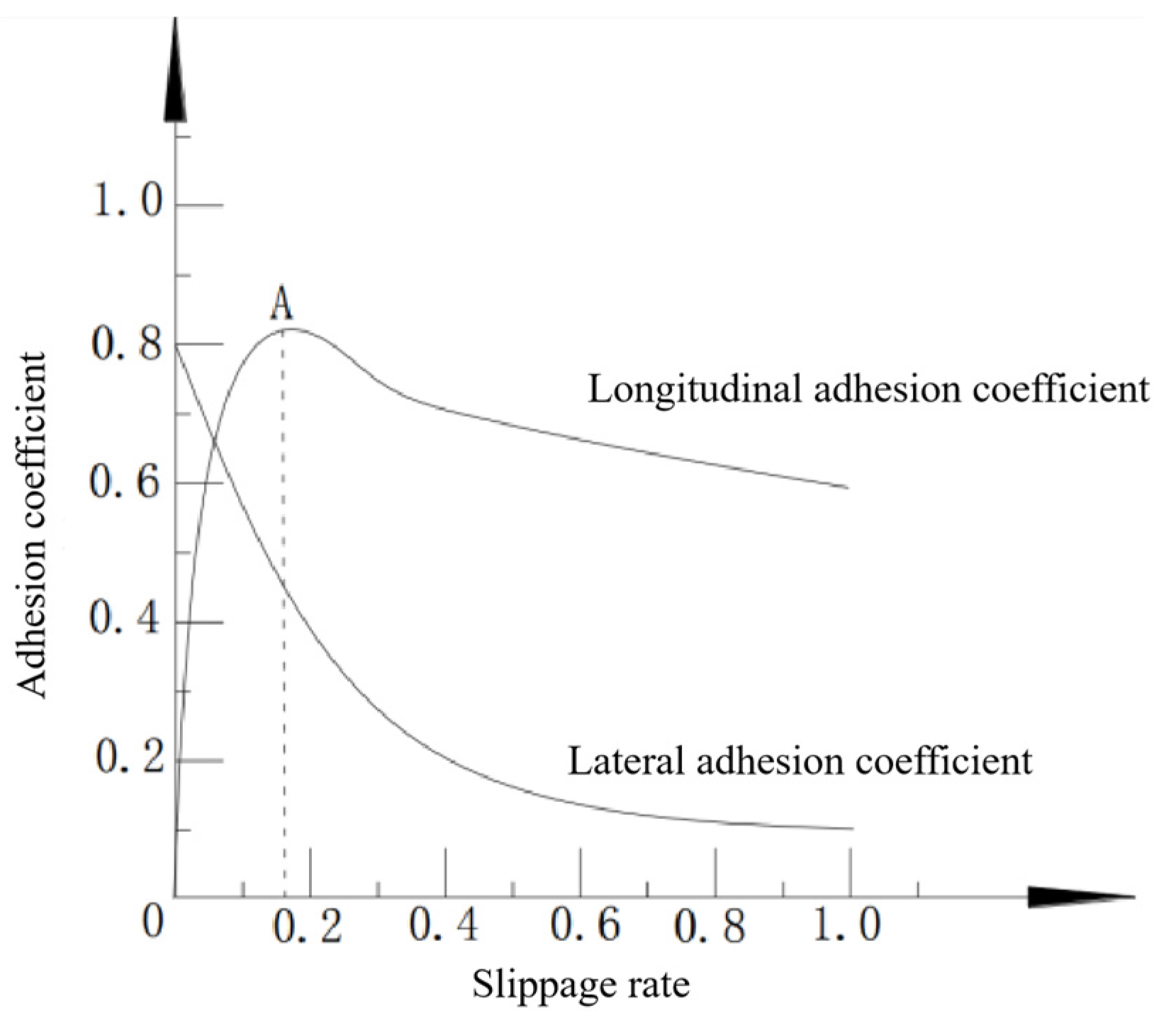
When the front-wheel drive vehicle is driving on a road with a low adhesion coefficient or turning at high speed, understeer occurs when the wheel slip rate is too large, causing the vehicle to lose maneuverability and stability. It can be seen from the curve of the adhesion coefficient and slip rate that understeer easily occurs when the lateral adhesion coefficient is minimal. Therefore, the goal of stability control is to ensure that the longitudinal coefficient of adhesion and lateral coefficient of adhesion are as significant as possible without losing the vehicle’s stability. As shown in Figure 4, when the slip rate reaches point A, the longitudinal adhesion coefficient reaches its maximum value. In contrast, the lateral adhesion coefficient corresponding to point A is small. If it continues to increase the slip rate, it will increase the risk of the vehicle losing stability.
4.2.1. Optimized Target Design
In order to ensure that the tires of a racing car have sufficient lateral stability margin to ensure the stability of the vehicle at high speeds and when cornering, minimum tire utilization is the control objective. Tire adhesion utilization refers to the ratio of the ground adhesion utilized by the tire to the maximum adhesion that the ground can provide, which can reflect the degree of stability of the vehicle. The higher the tire adhesion utilization rate, the higher the road adhesion rate utilized by the tire, and the lower the adhesion margin. When the adhesion utilization ratio is 1, it indicates that the tire is at the limit of adhesion, and the vehicle is at risk of destabilization at any time. On the contrary, the lower the tire adhesion utilization rate, indicating that the tire has more adhesion margin to resist external interference, the more stable the vehicle is.
At this time, the tire adhesion efficiency of the racing car is expressed as follows:
where , , and are the longitudinal, lateral, and vertical forces on the wheel of the racing car, respectively, and is the ground adhesion coefficient of the wheel.
Then, the stability margin of the tire can be expressed as
According to the tire friction ellipse principle, the lateral force available to the tire increases when the tire’s longitudinal force decreases. As shown in Figure 5, point a is the initial state working point of the tire; at this time, point a is inside the adhesion ellipse; the specific boundary has a certain distance; at this time, the tire longitudinal force and lateral force have more margin, and the vehicle is in a stable state of motion. The tire margin gradually decreases when moving from point a to point b. When reaching point b, the longitudinal and lateral forces of the tire reach the adhesion limit, and the vehicle is in a stable critical state. As the longitudinal force continues to increase until point c, the lateral force gradually decreases to 0. The available tire adhesion margin is tiny, and the vehicle is prone to understeer and oversteer.
With minimum tire utilization as the control objective, the objective function is shown in Equation (34):
where represents the tire utilization rate; represents the adhesion coefficient between the tire and the ground; represent the number of the four wheels of the racing car, i.e., left front, right front, left rear, and right rear, respectively; represents the longitudinal force of the tire; represents the lateral force of the tire; and represents the vertical load of the tire.
The estimation equation for the tire vertical load () is [36]
From Equation (35), it can be seen that when it is smaller, it represents the minimum amount of change required for the racing car to reach the target value from the current wheel longitudinal force under the same driving conditions, which in turn reduces the time for the vehicle to reach the target yaw moment and the motion response characteristics, so that the yaw motion response of the racing car is improved.
4.2.2. Torque Distribution Rules
In order to improve the stability of the front-wheel dual-motor-driven driverless racing car’s yaw stability during high-speed cornering, the formulation of a reasonable torque allocation rule is a critical and essential part [37]. Firstly, it is necessary to determine whether the current driving state of the racing car is an understeer state; secondly, it is essential to decide how to deal with the racing car when it is determined to be in the understeer state; and finally, it is required to distribute the torque according to the designed torque distribution rule. The direction of the additional yaw moment solved by the yaw moment controller, the direction of the actual front-wheel angle of the racing car, and the transverse angular velocity deviation are jointly used as the conditions for judging the driving state of a racing car. The yaw torque distribution method based on motor characteristics is used to convert the additional yaw torque required by the vehicle into driving or braking torque and control the car’s front wheel to increase the torque on one side of the motor and reduce the torque on the other. The torque distribution rules for the drive wheels are shown in Table 1:
The equation for the rotational dynamics of the wheel without considering the rolling resistance of the tire is
The constraints to be satisfied for each wheel drive torque are
where is the total demand torque; is the maximum torque output from the motor; and and are the left-front-wheel drive torque and right-front-wheel drive torque, respectively.
As a distributed drive structure, the torque of the front two drive wheels can be independently controlled, and the torque can be distributed and controlled in any proportion within the range of their torque capacity. This distributed drive arrangement structure provides feasibility for improving the stability and smoothness of the racing car when driving. According to the method of yaw moment distribution, when the racing car is steering, the inner wheel decreases the torque ΔT based on the average distribution torque, and the outer wheel increases the torque ΔT based on the average distribution torque.
The final outputs of the front inner and outer wheels after distribution can be obtained as follows:
where is the inner wheel torque of the front axle and is the outer wheel torque of the front axle.
5. Simulation and Result Analysis
A racing car stability control algorithm was built in MATLAB/Simulink, a racing car model was established in CarSim, and two typical test conditions were built. A joint simulation experiment platform of MATLAB/Simulink and CarSim was established to validate the driverless formula racing car yaw stability control strategy proposed in this paper. The particular parameters of the driverless formula racing car are shown in Table 2.
5.1. Double-Lane-Change (DLC) Simulation
The first simulation condition is the double-lane-change (DLC) condition. According to the driverless system recognizing the double-lane-change path trajectory as the steering wheel angle input, in order to simulate the race track road conditions, we selected the adhesion coefficient (μ) for 1.0, and according to the double-lane-change trajectory planning for the driving speed of the car’s expected speed, in Carsim, we set the expected speed to 60 km/h. The joint simulation results are shown in Figure 6.
From Figure 6, the stability of the driverless formula racing car during the double-lane-change test can be more significantly improved by adding the yaw moment controller.
Figure 6a, b show the expected traverse yaw angular velocity as the observation target. The performance of the transverse yaw moment controller is evaluated by judging the deviation of the vehicle’s actual transverse yaw angular velocity from the expected yaw velocity. It can be seen that the yaw moment controller can control the vehicle tracking on the expected yaw angular velocity to minimize the resulting yaw angular velocity error when the vehicle yaw angular velocity changes abruptly. Figure 6a shows that when the vehicle moves under double-shift working conditions, the maximum value of the expected yaw angular velocity is 2.082 dag/s. Without yaw torque control, the absolute value of the maximum yaw angular velocity generated is 2.808 dag/s. After adding the yaw torque controller, the absolute value of the maximum yaw torque generated is reduced to 2.285 dag/s. Meanwhile, according to Figure 6b, it can be seen that when no yaw moment control is performed, the resulting maximum yaw moment error is 1.663 dag/s. In contrast, the maximum yaw moment error is reduced to 0.602 dag/s after adding yaw moment control, and the yaw moment error is reduced by 63%.
The performance of the yaw moment controller is evaluated by judging the deviation of the vehicle’s actual side slip angle from the expected side slip angle. It can be seen that the yaw moment controller plays a specific role in controlling the vehicle’s side slip angle, which helps improve the vehicle’s stability during cornering. From Figure 6c, d, it can be seen that the maximum side slip angle error generated without yaw moment control is 0.1256 dag. In contrast, the maximum yaw moment error is reduced to 0.0418 dag after adding yaw moment control, and the yaw moment error is reduced by 66.7%.
In summary, it can be seen that the vehicle with the function of yaw torque control is better than the vehicle without yaw torque control in the control of yaw angular velocity and side slip angle, and the designed yaw torque controller can improve the driving stability of the vehicle under this working condition.
5.2. Autocross Traction Simulation
In order to more intuitively see the operating effect of the yaw moment controller designed in this paper in an actual race situation, a part of the high-speed tracking program track with many curves is intercepted as the target path, as shown in Figure 7. The road trajectory recognized by the unmanned system is used as the steering wheel angle input, and the road surface adhesion coefficient is set to 0.4 to simulate wet race track road surface after rainfall. The simulation speed should also be the driving speed planned according to the double-shift trajectory, and the expected speed of the uncrewed racing car is set to 60 km/h. The simulation results are shown in Figure 8.
The simulation results are shown in Figure 8. The driverless formula car with yaw stability controller has good stability control ability on the high-speed tracking multi-curve road under the condition of ground adhesion coefficient, and it can effectively control the yaw angle and the center of mass side deviation angle to ensure the smooth driving of the car.
As can be seen in Figure 8a, when the car enters this autocross tracking course at a speed of 60 km/h on the curved section, the yaw angle of the car can be closer to the expected yaw angle after adding yaw torque control than when it is not controlled. However, as can be seen in Figure 8b, when the car does not have yaw torque control, the maximum yaw angle error is 0.1262 dag, while the maximum yaw angle error is reduced to 0.0847 dag/s after adding yaw torque control, and the yaw angle error is reduced by 32%, which is a significant reduction in error. Figure 8c, d takes the side slip angle and the side slip angle error as the tracking targets, and it can be seen in the two subfigures that after adding the yaw moment controller, the max side slip angle error is reduced from 1.341 to 0.048, which is a 63.6% reduction, when the racing car is driving on this low-adhesion-coefficient section. It shows that the yaw moment controller designed in this paper can improve the yaw stability of the driverless formula racing car while driving on the actual low-adhesion-coefficient autocross track, which also proves the effectiveness of the yaw stability controller.
6. Conclusions
This paper proposes a stability control strategy for a front-wheel dual-motor-driven driverless formula racing car. The following conclusions are drawn:
- Taking the yaw stability of the racing car as the control objective, the upper layer is designed based on integral sliding mode theory, which solves the jitter problem of the traditional sliding mode control by introducing an integral term based on the original sliding mode control principle. The linear two-degree-of-freedom model of the racing car is established to calculate the expected yaw angular velocity, the expected side slip angle, and the additional yaw moment.
- Aiming at the additional torque generated when the racing car turns, the lower torque distribution controller is designed, and the torque optimization goal and torque distribution rules of the car are used as the evaluation criteria to optimize the torque distribution of the two motors of the inner and outer wheels.
- The results of simulation experiments under two different working conditions show that the yaw stability of the driverless formula racing car with the yaw stability control strategy proposed in this paper is significantly improved when traveling and turning under different road conditions, which verifies the effectiveness of the yaw stability control strategy proposed in this paper. It improves the yaw stability of the car when turning at high speed and driving on low-adhesion-coefficient roads.
Author Contributions
Conceptualization, B.L. and G.L.; methodology, B.L. and H.B.; software, S.W. and B.L.; validation, B.L., G.L., H.B. and X.Z.; formal analysis, B.L.; investigation, H.B.; resources, G.L.; data curation, S.W. and X.Z.; writing—original draft preparation, B.L.; writing—review and editing, B.L. and G.L.; visualization, B.L. and S.W.; supervision, G.L.; project administration, G.L.; funding acquisition, G.L. and B.L. All authors have read and agreed to the published version of the manuscript.
Funding
This research was funded by the General Program of the Natural Science Foundation of Liaoning Province in 2022 (2022-MS-376) and the Natural Science Foundation joint fund project (U22A2043).
Data Availability Statement
The data used to support the findings of this study are available from the corresponding author upon request.
Conflicts of Interest
The authors declare no conflicts of interest.
References
- Hu, J. Rules for China University Student Driverless Formula Competition. Available online: http://www.formulastudent.com.cn/news/5770.html (accessed on 18 April 2024).
- Zhang, Z.; Li, G.; Li, N. Research on cooperative control strategy of FSAC racing car trajectory tracking. J. Automot. Eng. 2023, 13, 750–759. [Google Scholar] [CrossRef]
- Li, X.; Yin, G.; Ren, Y.; Wang, F.; Fang, R.; Li, A. Hierarchical Control for Distributed Drive Electric Vehicles Considering Handling Stability and Energy Efficiency. In Proceedings of the 2023 IEEE International Automated Vehicle Validation Conference (IAVVC), Austin, TX, USA, 16–18 October 2023; pp. 1–6. [Google Scholar] [CrossRef]
- Feng, Y.; Zhang, B.; Zhang, R.; Shi, P.; Wang, Z.; Zhou, C. Estimations of vehicle driving state and road friction coefficient based on High-degree cubature Kalman filter of distributed drive electric vehicles. In Proceedings of the 2021 5th CAA International Conference on Vehicular Control and Intelligence (CVCI), Tianjin, China, 29–31 October 2021; pp. 1–6. [Google Scholar] [CrossRef]
- Yu, C.; Zheng, Y.; Shyrokau, B.; Ivanov, V. MPC-based Path Following Design for Automated Vehicles with Rear Wheel Steering. In Proceedings of the 2021 IEEE International Conference on Mechatronics (ICM), Kashiwa, Japan, 7–9 March 2021; pp. 1–6. [Google Scholar] [CrossRef]
- Mutoh, N.; Saitoh, T.; Sasaki, Y. Driving Force Control Method to Perform Slip Control in Cooperation with the Front and Rear Wheels for Front-and-Rear Wheel-Independent-Drive-Type EVs (FRID EVs). In Proceedings of the 2008 11th International IEEE Conference on Intelligent Transportation Systems, Beijing, China, 12–15 October 2008; pp. 925–930. [Google Scholar] [CrossRef]
- Woo, S. Active Differential Control for Improved Handling Performance of Front-Wheel-Drive High-Performance Vehicles. Int. J. Automot. Technol. 2021, 22, 537–546. [Google Scholar] [CrossRef]
- Liang, Z.; Shen, M.; Zhao, J.; Li, Z.; Wang, Y.; Ding, Z. Adaptive Sliding Mode Fault Tolerant Control for Autonomous Vehicle With Unknown Actuator Parameters and Saturated Tire Force Based on the Center of Percussion. IEEE Trans. Intell. Transp. Syst. 2023, 24, 11595–11606. [Google Scholar] [CrossRef]
- Sakhnevych, A.; Arricale, V.M.; Bruschetta, M.; Censi, A.; Mion, E.; Picotti, E.; Frazzoli, E. Investigation on the Model-Based Control Performance in Vehicle Safety Critical Scenarios with Varying Tyre Limits. Sensors 2021, 21, 5372. [Google Scholar] [CrossRef] [PubMed]
- Song, Y.; Shu, H.; Chen, X.; Luo, S. Direct-yaw-moment control of four-wheel-drive electrical vehicle based on lateral tyre–road forces and sideslip angle observer. IET Intell. Transp. Syst. 2019, 13, 303–312. [Google Scholar] [CrossRef]
- Liu, Z.; Qiao, Y.; Chen, X. A Novel Control Strategy of Straight-line Driving Stability for 4WID Electric Vehicles Based on Sliding Mode Control. In Proceedings of the 2021 5th CAA International Conference on Vehicular Control and Intelligence (CVCI), Tianjin, China, 29–31 October 2021; pp. 1–6. [Google Scholar] [CrossRef]
- Li, Z.; Wang, P.; Chen, H. Coordinated longitudinal and lateral vehicle stability control based on the combined-slip tire model in the MPC framework. In Proceedings of the 2020 Chinese Control And Decision Conference (CCDC), Hefei, China, 22–24 August 2020; pp. 103–105. [Google Scholar] [CrossRef]
- Chu, L.; Chen, J.; Yao, L.; Chao, L.; Zhang, Y.; Liu, M.; Zhao, Z. Vehicle stability control algorithm based on optimal fuzzy theory. In Proceedings of the 2011 International Conference on Electronic & Mechanical Engineering and Information Technology, Harbin, China, 12–14 August 2011; pp. 3210–3213. [Google Scholar] [CrossRef]
- Li, Q.; Li, J.; Wang, S.; Zhang, X.; Liu, J. Four Wheel Steering Vehicles Stability Control Based on Adaptive Radial Basis Function Neural Network. In Proceedings of the 2021 33rd Chinese Control and Decision Conference (CCDC), Kunming, China, 22–24 May 2021; pp. 1140–1145. [Google Scholar] [CrossRef]
- Saikia, A.; Mahanta, C. Vehicle stability enhancement using sliding mode based active front steering and direct yaw moment control. In Proceedings of the 2017 Indian Control Conference (ICC), Guwahati, India, 4–6 January 2017; pp. 378–384. [Google Scholar] [CrossRef]
- Cai, L.; Liao, Z.; Wei, S.; Li, J. Improvement of Maneuverability and Stability for Eight wheel Independently Driven Electric Vehicles by Direct Yaw Moment Control. In Proceedings of the IEEE 2021 24th International Conference on Electrical Machines and Systems (ICEMS), Gyeongju, Republic of Korea, 31 October 2021–3 November 2021. [Google Scholar] [CrossRef]
- Zhou, H.; Chen, H.; Ren, B.; Zhao, H. Yaw stability control for in-wheel-motored electric vehicle with a fuzzy PID method. In Proceedings of the 27th Chinese Control and Decision Conference (2015 CCDC), Qingdao, China, 23–25 May 2015; pp. 1876–1881. [Google Scholar] [CrossRef]
- Kong, D.; Liu, C.; Cui, M.; Lv, Y.; Liu, K.; Guo, H. Yaw Stability Control of Distributed Drive Electric Vehicle Based on Torque Optimal Distribution in Ice and Snow Environment. In Proceedings of the IEEE 2022 6th CAA International Conference on Vehicular Control and Intelligence (CVCI), Nanjing, China, 28–30 October 2022. [Google Scholar] [CrossRef]
- Wang, S.; Zhang, J. The research and application of fuzzy control in four-wheel-steering vehicle. In Proceedings of the 2010 Seventh International Conference on Fuzzy Systems and Knowledge Discovery, Yantai, China, 10–12 August 2010; Volume 3, pp. 1397–1401. [Google Scholar] [CrossRef]
- Zhang, H.; Xu, D.; Li, Y.; Hu, X. Fuzzy neural network simulation of vehicle yaw rate control based on PID. In Proceedings of the 2020 3rd World Conference on Mechanical Engineering and Intelligent Manufacturing (WCMEIM), Shanghai, China, 4–6 December 2020; pp. 430–434. [Google Scholar] [CrossRef]
- Li, Y.; Huang, P.; Xie, T. A Research on Adaptive Neural Network Control Strategy of Vehicle Yaw Stability. In Proceedings of the 2013 Fourth International Conference on Intelligent Systems Design and Engineering Applications, Zhangjiajie, China, 6–7 November 2013; pp. 48–51. [Google Scholar] [CrossRef]
- Bhoi, S.C.; Swain, S.K. Sliding Mode Based Robust Lateral Control for Autonomous Vehicles. In Proceedings of the 2021 International Symposium of Asian Control Association on Intelligent Robotics and Industrial Automation (IRIA), Goa, India, 20–22 September 2021; pp. 222–227. [Google Scholar] [CrossRef]
- Saepulah, F.; Santoso, A. Electric Vehicle Lateral Stability Control Design Based on Brake-By-Wire System Using Fuzzy-SMC. In Proceedings of the 2022 2nd International Seminar on Machine Learning, Optimization, and Data Science (ISMODE), Jakarta, Indonesia, 22–23 December 2022; pp. 385–390. [Google Scholar] [CrossRef]
- Ahn, T.; Lee, Y.; Park, K. Design of Integrated Autonomous Driving Control System That Incorporates Chassis Controllers for Improving Path Tracking Performance and Vehicle Stability. Electronics 2021, 10, 144. [Google Scholar] [CrossRef]
- Zhao, J.; Chen, J.; Liu, C. Stability Coordinated Control of Distributed Drive Electric Vehicle Based on Condition Switching. Math. Probl. Eng. 2020, 2020, 5648058. [Google Scholar] [CrossRef]
- Tian, T.; Fang, L.; Ding, S.; Zheng, W.X. Adaptive Fuzzy Sliding Mode Control for Active Front Steering System. In Proceedings of the 2020 39th Chinese Control Conference (CCC), Shenyang, China, 27–29 July 2020; pp. 358–363. [Google Scholar] [CrossRef]
- Hajjami, L.; Mellouli, E.M.; Berrada, M. Robust adaptive non-singular fast terminal sliding-mode lateral control for an uncertain ego vehicle at the lane-change maneuver subjected to abrupt change. Int. J. Dyn. Control 2021, 9, 1765–1782. [Google Scholar] [CrossRef]
- Guo, J.; Wang, J. Lateral stability control of distributed drive electric vehicle based on fuzzy sliding mode contro. In Proceedings of the 2017 IEEE 3rd Information Technology and Mechatronics Engineering Conference (ITOEC), Chongqing, China, 3–5 October 2017; pp. 675–680. [Google Scholar] [CrossRef]
- Wang, S.; Zhao, X.; Yu, Q.; Yu, M. Stability control strategy of electric vehicle with dual-motor drive based on driver’s steering intention. China Highw. J. 2022, 35, 334–349. [Google Scholar] [CrossRef]
- Rajamani, R. Vehicle Dynamics and Control; Springer Science & Business Media: New York, NY, USA, 2012. [Google Scholar] [CrossRef]
- Edwards, C.; Sarah, K. Sliding Mode Control: Theory and Applications; Crc Press: London, UK, 1998. [Google Scholar] [CrossRef]
- Chen, Z.; Gao, Q.; Tan, L. Adaptive Backstepping Sliding-Mode Control for Permanent Magnet Linear Synchronous Motors. In Proceedings of the 2018 37th Chinese Control Conference (CCC), Wuhan, China, 25–27 July 2018; pp. 2690–2693. [Google Scholar] [CrossRef]
- Patil, H.; Devika, K.B.; Vivekanandan, G.; Sivaram, S.; Subramanian, S.C. Direct yaw-moment control integrated with wheel slip regulation for heavy commercial road vehicles. IEEE Access 2022, 10, 69883–69895. [Google Scholar] [CrossRef]
- Bai, Y.; Li, G.; Jin, H.; Li, N. Research on Lateral and Longitudinal Coordinated Control of Distributed Driven Driverless Formula Racing Car under High-Speed Tracking Conditions. J. Adv. Transp. 2022, 2022, 7344044. [Google Scholar] [CrossRef]
- Zhao, F.; An, J.; Chen, Q.; Li, Y. Integrated Path Following and Lateral Stability Control of Distributed Drive Autonomous Unmanned Vehicle. World Electr. Veh. J. 2024, 15, 122. [Google Scholar] [CrossRef]
- Zhang, B.; Chen, Z.; Fu, J.; Chen, B. Adaptive drive skid control for four-wheel independent drive electric vehicles. J. Shandong Univ. (Eng. Ed.) 2018, 48, 96–103. [Google Scholar] [CrossRef]
- Ni, J.; Hu, J.; Xiang, C. Robust path following control at driving/handling limits of an autonomous electric racecar. IEEE Trans. Veh. Technol. 2019, 68, 5518–5526. [Google Scholar] [CrossRef]
Figure 1.
Principle of yaw stability control.
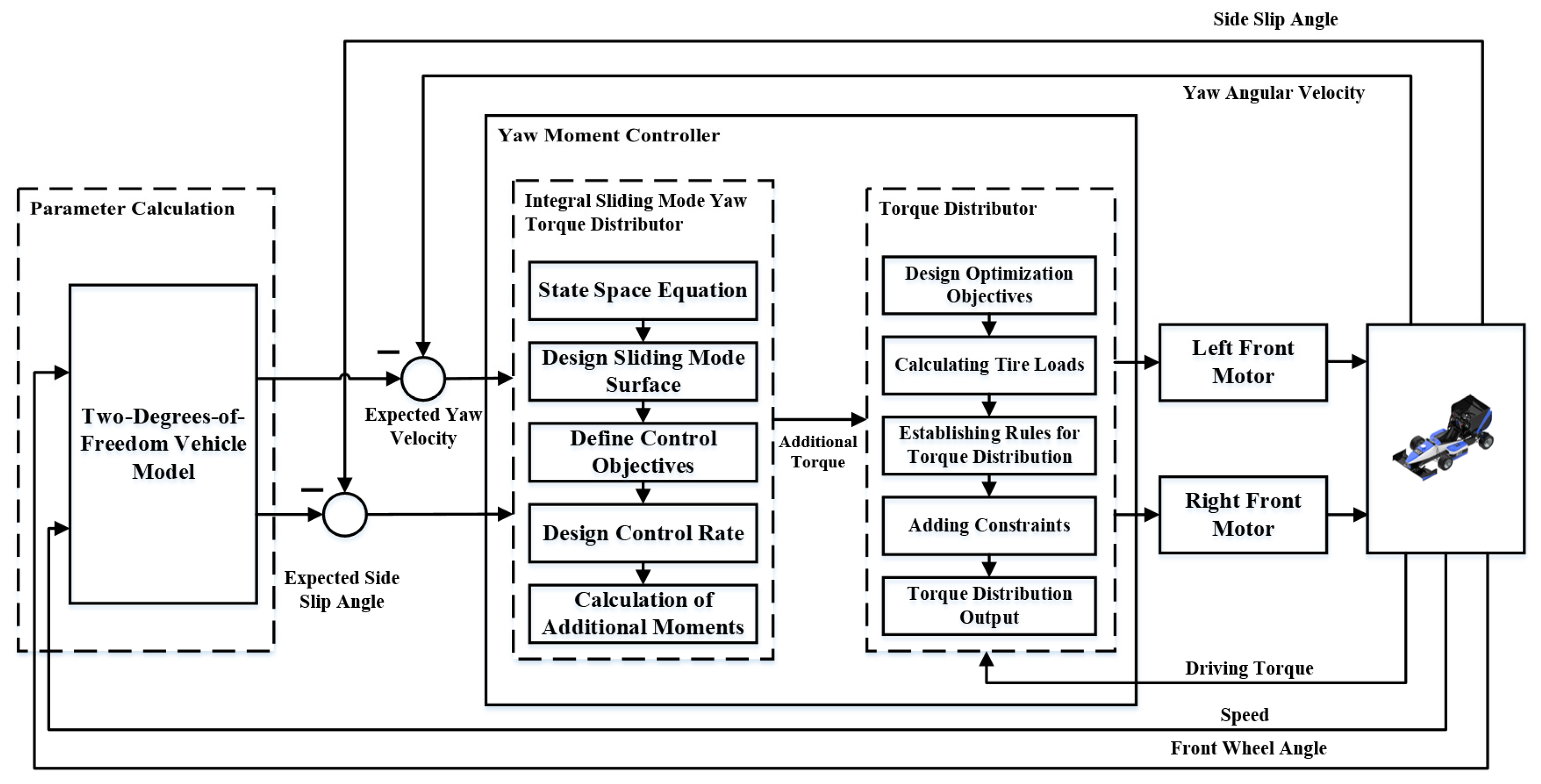
Figure 2.
Two-degree-of-freedom vehicle dynamics model.
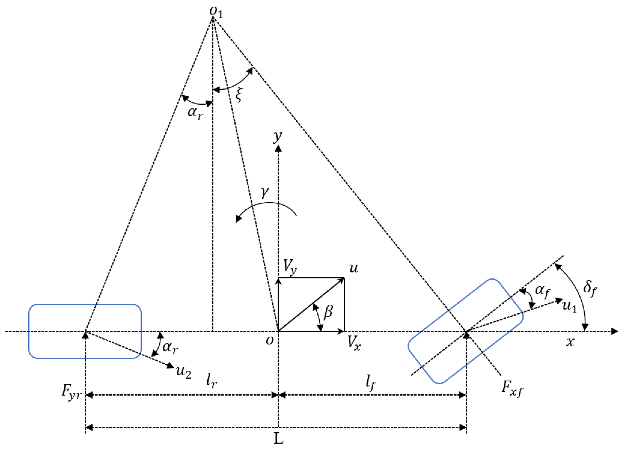
Figure 3.
Characterization of the three points on the switching plane.

Figure 4.
Relationship between slip rate and adhesion coefficient.

Figure 5.
Adhesion ellipse model.
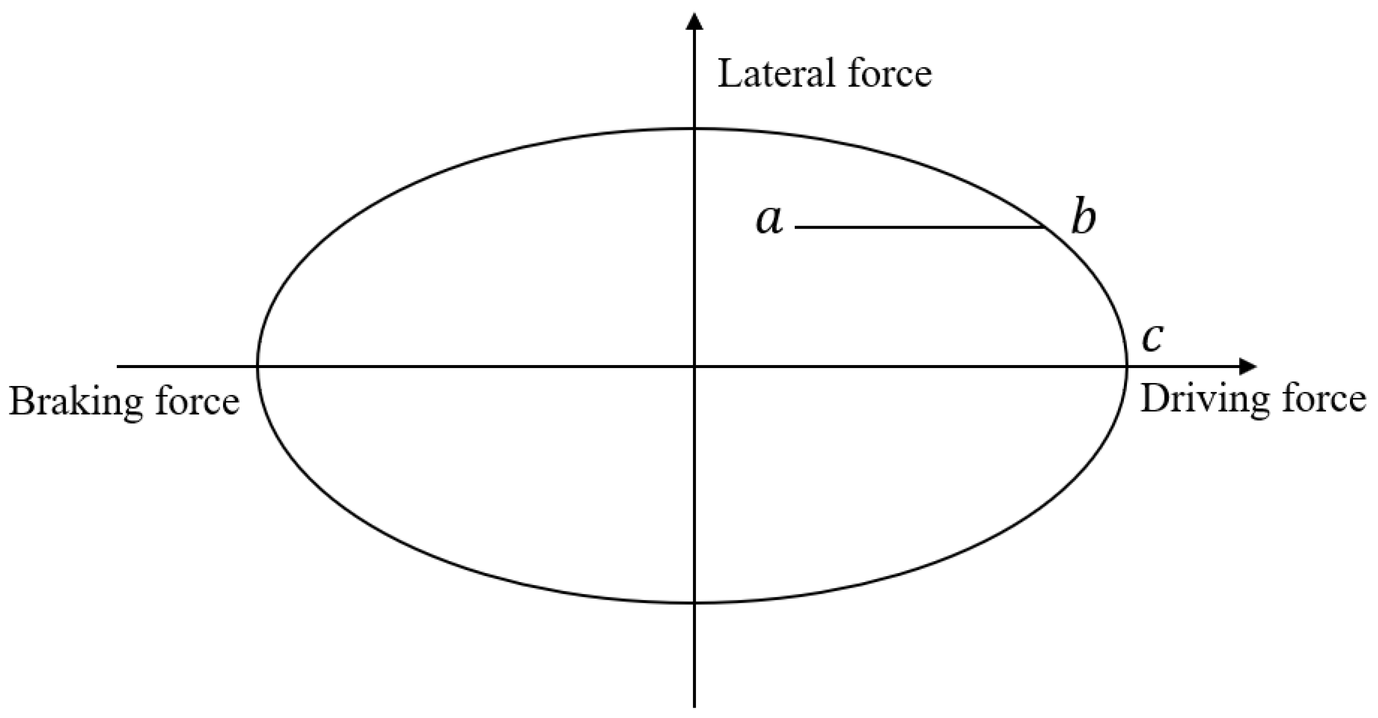
Figure 6.
Comparison of double-shift working condition: (a) yaw angular velocity; (b) yaw velocity error; (c) side slip angle; (d) side slip angle error.
Figure 6.
Comparison of double-shift working condition: (a) yaw angular velocity; (b) yaw velocity error; (c) side slip angle; (d) side slip angle error.

Figure 7.
Autocross tracking path.
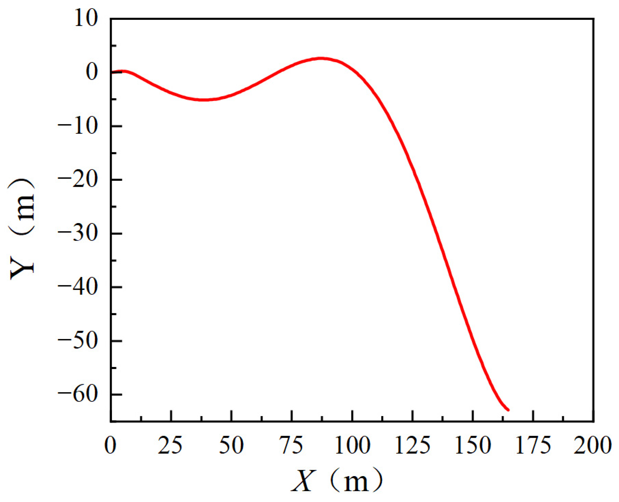
Figure 8.
Autocross traction comparison: (a) yaw angle; (b) yaw angular error; (c) side slip angle; (d) side slip angle error.
Figure 8.
Autocross traction comparison: (a) yaw angle; (b) yaw angular error; (c) side slip angle; (d) side slip angle error.


Table 1.
Wheel torque distribution rules.
| Steering | Front-Wheel Steering Angle | Yaw Velocity Deviation | Additional Yaw Moment | Steering Characteristic | Torque Distribution |
|---|---|---|---|---|---|
| Left turn | Oversteer | ||||
| Left turn | Understeer | ||||
| Right turn | Understeer | ||||
| Right turn | Oversteer |
Table 2.
Basic parameters of the racing car.
| Symbol | Definition | Value |
|---|---|---|
| m | Vehicle mass | 260 kg |
| a | Distance of CG from front axle | 760.5 mm |
| b | Distance of CG from rear axle | 852.5 mm |
| c | Wheelbase | 1210 mm |
| l | Axle base | 1550 mm |
| h | Height of CG | 300 mm |
| Iz | Vehicle yaw moment of inertia | 1325 kg/m2 |
| J | Wheel yaw moment of inertia | 0.9 kg/m2 |
Disclaimer/Publisher’s Note: The statements, opinions and data contained in all publications are solely those of the individual author(s) and contributor(s) and not of MDPI and/or the editor(s). MDPI and/or the editor(s) disclaim responsibility for any injury to people or property resulting from any ideas, methods, instructions or products referred to in the content. |
© 2024 by the authors. Licensee MDPI, Basel, Switzerland. This article is an open access article distributed under the terms and conditions of the Creative Commons Attribution (CC BY) license (https://creativecommons.org/licenses/by/4.0/).
Share and Cite
MDPI and ACS Style
Liu, B.; Li, G.; Bai, H.; Wang, S.; Zhang, X. Research on Yaw Stability Control of Front-Wheel Dual-Motor-Driven Driverless Formula Racing Car. World Electr. Veh. J. 2024, 15, 178. https://doi.org/10.3390/wevj15050178
AMA Style
Liu B, Li G, Bai H, Wang S, Zhang X. Research on Yaw Stability Control of Front-Wheel Dual-Motor-Driven Driverless Formula Racing Car. World Electric Vehicle Journal. 2024; 15(5):178. https://doi.org/10.3390/wevj15050178
Chicago/Turabian StyleLiu, Boju, Gang Li, Hongfei Bai, Shuang Wang, and Xing Zhang. 2024. "Research on Yaw Stability Control of Front-Wheel Dual-Motor-Driven Driverless Formula Racing Car" World Electric Vehicle Journal 15, no. 5: 178. https://doi.org/10.3390/wevj15050178