Charging Station Site Selection Optimization for Electric Logistics Vehicles, Taking into Account Time-Window and Load Constraints

Abstract

In order to improve the efficiency of the “last-mile” distribution in urban logistics and solve the problem of the difficult charging of electric logistics vehicles (ELVs), this paper proposes a charging station location optimization scheme for ELVs that takes into account time-window and load constraints (TW-LCs). Taking the optimal transportation path as the objective function and considering the time-window and vehicle load constraints, a charging station siting model was established. For the TW-LC problem, an improved genetic algorithm combining the farthest-insertion heuristic idea and local search operation was designed. Three different types of standardized arithmetic examples, C type, R type, and RC type, were used to test the proposed algorithm and compare it with the traditional genetic algorithm. The results indicate that, under the same conditions, compared to the traditional genetic algorithm, the improved genetic algorithm reduced the optimal path length by an average of 11.12%. It also decreased the number of charging stations selected, the number of vehicles in use, and the algorithm complexity by 22.97%, 13.71%, and 46.81%. Building on this, a case study was conducted on the TW-LC problem in a specific area of Chongqing, China. It resulted in a 50% reduction in the number of charging stations and a 25% reduction in the number of vehicles selected. In terms of economic indicators, the proposed algorithm improves unit electricity sales by 73.88% and reduces the total annualized cost of the logistics company by 18.81%, providing a theoretical basis for the subsequent promotion of ELVs.

1. Introduction

Excessive carbon emissions cause environmental pollution and accelerate global warming. In recent years, decision makers in logistics companies have been paying more attention to the concept of green transportation [1]. In 2023, global electric vehicle ownership reached 117 million units, up 44.36% from 81.05 million units in 2022. Global sales of electric vehicles are expected to exceed 70 million units in 2030, when ownership will reach 380 million units and penetration will reach 60%. Advance planning for the locations of charging stations for ELVs is an important process for the future development of ELVs. A charging station consists of solid-state transformers and other equipment, and a reasonable charging facility layout can reduce power electronic requirements and facilitate grid power dispatch [2,3]. In addition to this, it can also reduce the construction and operating costs of charging stations for operators, ease the charging anxiety of delivery workers, reduce the time spent looking for charging stations, improve delivery efficiency, and increase customer satisfaction [4]. Therefore, it is of great significance to optimize the site selection of charging stations for ELVs.

Charging station siting optimization for ELVs involves vehicle path planning and charging station siting, i.e., the Location-Routing Problem (LRP) [5,6]. In response to this problem, Dan Wang et al. [7] proposed a site selection scheme based on an adaptive large neighborhood search for ELVs under uncertain power consumption. The total cost was used as the objective function, and local search operations were incorporated while using the new operator. A case analysis showed that the scheme improves the search capability of the model, enhances the stability of site selection, reduces the construction cost of charging piles, and optimizes the site selection problem in the case of the fluctuating power consumption of ELVs. Yang Senyan et al. [8] developed a charging station siting model for ELVs with a hybrid recycling strategy and a charging strategy. The charging station construction cost was minimized as an objective function and solved using hybrid Lagrangian relaxation and alternating-direction multiplier methods. The results show that the scheme balances the complexity of the model with the solution time. Zhao Jiao et al. [9], based on a genetic algorithm, added a greedy search strategy and an elite retention strategy to minimize the total cost as an objective function to solve the siting model considering the charging queuing time of ELVs. The solution results show that the scheme reduces the cost of siting the charging station and shortens the waiting time when charging ELVs. Selin Hulagu et al. [10] proposed a site selection–path planning scheme based on the energy consumption and recovery of ELVs in different scenarios, with cost minimization as the objective function. The results of an arithmetic example showed that this siting scheme is more reliable in areas with significant elevation changes. B Praveen Kumar et al. [11] used Dijkstra’s algorithm combined with an LSTM deep learning model to plan vehicle paths using the shortest vehicle path as the objective function. An example analysis showed that the algorithm effectively reduces the distance traveled by the vehicle. Vidhya Kannan et al. [12] proposed a Bellman–Ford algorithm with a score function to solve the vehicle shortest path planning problem in road networks. Updating the weights based on the score of the evaluation function effectively reduces the vehicle travel distance.

In the LRP, it is path planning that dominates the decision on siting. Using the cost as an objective function often does not accurately reflect the vehicle paths, resulting in a non-optimal solution for performing site selection. And in a multi-node, multi-objective, large-scale optimization problem, using cost as the objective function often makes convergence difficult, and the solution speed is slow [13].

Due to the existence of logistics and distribution characteristics such as timeliness, a common treatment scheme involves adding time-window constraints to the model. Wang Yong et al. [14] designed a combination of a Gaussian hybrid clustering algorithm and an improved non-dominated sorting genetic algorithm with total cost minimization as the objective function. Concepts such as time windows for users and resource sharing have been added to the constraints. An example study of the ELV siting–path problem for a site in Chongqing, China, showed that the scheme improves the operational efficiency of the logistics network and the utilization of resources. Li-Ying Song et al. [15] proposed a hybrid fleet cold chain logistics distribution path optimization problem considering carbon emissions and the customer time window, which rationally allocates the ratios of fuel and ELVs in the fleet, optimizes the charging time of the trams and the refueling time of the oil trucks, and meets the constraints of the time window of the customer points in different regions.

Logistics transportation, in addition to considering time-window constraints, should also consider vehicle load constraints in order to rationalize the arrangement of vehicles to serve customers with different demand points [16].

In summary, when studying the problem of siting charging stations for ELVs, there are situations such as a non-optimal objective function and the incomplete consideration of constraints. Therefore, this paper proposes a charging station location optimization scheme for ELVs that takes into account time-window and load constraints, where the optimal path is used as the objective function and time-window and load constraints are added to the transportation paths. The solution aims to reduce the number of charging stations selected and reduce the number of vehicles in use while optimizing distribution paths and improving distribution efficiency.

2. Problem Description and Problem Formulation

2.1. TW-LC Problem Description

TW-LCs mean that there are a certain number of customer points, which have different time windows and different amounts of cargo demand, and the ELV is responsible for distributing the cargo from the distribution center. By organizing appropriate routes, it traverses all customer points and selects the optimal path between them. At the same time, we also need to satisfy the time-window constraints of the customer points and the load constraints of the vehicles, and according to the power consumption of the ELV, we can reasonably set up charging stations on the transportation route.

The charging station siting model for ELVs proposed in this paper can include a distribution center involving multiple ELVs, multiple locations for constructing charging stations, and multiple customer locations. The ELV starts at the distribution center, goes through a number of customer points, and finally returns to the starting point. On the way, it passes through a charging station to replenish its power, and each time it is replenished, it is fully charged. The time window for the customer points is a soft time window, and there are penalties for being earlier or later than the time window. The TW-LC problem is shown in Figure 1.

The transportation scenario proposed in this paper has the following assumptions: (1) There is no delivery demand at the charging station, so the demand is 0. (2) The ELV will not visit the next charging station immediately after visiting one charging station. (3) The driving speed of the ELV is uniform. (4) Each charging station has a sufficient number of charging posts. (5) The ELV does not consume power when it stops at a customer point.

2.2. Linear Programming Optimization Model

The definition of sets and variables in the charging station siting model for ELVs established in this paper is detailed in

Table 1. Notation for the TW-LC problem.

Sets and Variables	Meaning
A	Set of nodes
K	Set of vehicles
N	Set of client points to be served
D	Set of distribution centers
E	Set of charging stations
$x_{i\theta k}$	0–1 variable: 1 when the program serves client point i and 0 otherwise
$x_{ijk}$	0–1 variable: 1 when the vehicle goes from i to j and 0 otherwise
$x_{iDk}$	0–1 variable: 1 when the vehicle departs from the distribution center and finally returns to the distribution center and 0 otherwise
$x_{D\eta k}$	0–1 variable: 0 when the vehicle is charged immediately after departure from the distribution center and 1 otherwise

.

2.2.1. Optimal Path Objective Function Design

Equation (1) represents the optimal path, which consists of the total distance traveled by the ELV, the sum of the capacity constraints violated by each path, the sum of the load constraints violated by all the customer points, the sum of the power consumption constraints violated by all the vehicles, and four variables. $\alpha$, $\beta$, and $\gamma$ are coefficients. Since load constraints are relatively difficult to violate, $\alpha$ is set to 10. The time-window and power consumption constraints are easier to violate, so $\beta$ and $\gamma$ are set to 100. $d_{ij}$ denotes the distance from client point i to client point j; and q represents the synthesis of load constraint violations; $t_{ik}$ represents the time when vehicle k arrives at customer point j; $l_i$ represents the right time window of client point i, i.e., the latest expected arrival time of client point i; g represents the synthesis of the power consumption constraint violation.

$$OP=\sum _{i\in A}\sum _{j\in A,i\ne j}\sum _{k\in K}{d}_{ij}{x}_{ijk}+\alpha q+\beta \sum _{i=1}^{n}max\left\{\left(t_{ik}-l_i\right),0\right\}+\gamma g$$

(1)

2.2.2. Restrictive Conditions

Load constraints: Equation (2) indicates that the total weight of the goods carried by the vehicle does not exceed the maximum load capacity. $Q_{\theta }$ represents the demand for goods at customer point $\theta$ to be served; and C indicates the rated load capacity of the ELV.

$$\sum _{i\in A,i\ne \theta }\sum _{\theta \in N}{Q}_{\theta }{x}_{i\theta k}\le C,\forall k\in K$$

(2)

Path constraints: Equation (3) represents the conservation of traffic flow at each node, i.e., vehicles entering are equal to vehicles exiting; Equation (4) indicates that each client point should be visited and only once; Equation (5) indicates that all ELVs depart from the distribution center only once; Equation (6) represents the elimination of sub-loop constraints; and Equations (7) and (8) indicate that the ELV departs from the distribution center and finally returns to the distribution center.

$$\sum _{i\in A,i\ne j}{x}_{ijk}=\sum _{j\in A,j\ne i}{x}_{jik}$$

(3)

$$\sum _{i\in A,i\ne \theta }\sum _{k\in K}{x}_{i\theta k}=\sum _{i\in A,i\ne \theta }\sum _{k\in K}{x}_{\theta ik}=1,\forall \theta \in N$$

(4)

$$\sum _{j\in A}{x}_{Djk}=\sum _{j\in A}{x}_{jDk}\le 1,\forall k\in K$$

(5)

$$\sum _{i\in A}\sum _{j\notin A}{x}_{ij}\ge 1,A\subset N,A\ne ⌀$$

(6)

$$\sum _{j\in A}{x}_{Djk}=1,\forall k\in K$$

(7)

$$\sum _{i\in A}{x}_{i{D}^{\prime }k}=1,\forall k\in K$$

(8)

Power consumption constraints: Equation (9) indicates that charging is required when the remaining power of the vehicle is less than e, which is set to 0.2; $\lambda$ is the percentage of power consumption per 1 mile traveled by the ELV, which is set to 0.32%; S denotes the percentage of remaining power; and L denotes the distance traveled by the vehicle since the last charging. Equation (10) indicates that the vehicle will not be charged immediately after departure from the distribution center. Equations (11) and (12) represent the state of the vehicle when it departs from the distribution center and the charging station. $P_{BDk}$ indicates that the vehicle was fully charged when it departed from the distribution center; $P_{B\eta k}$ indicates that the vehicle was fully charged when it departed from the charging station; and F indicates that the vehicle’s battery status was fully charged. Equation (13) indicates that the remaining power of the vehicle remains unchanged before and after visiting the customer point.

$$S=1-\lambda L\ge e$$

(9)

$$x_{D\eta k}=0,\forall \eta \in E,\forall k\in K$$

(10)

$$P_{BDk}=F,\forall k\in K$$

(11)

$$P_{B\eta k}=F,\forall \eta \in E,\forall k\in K$$

(12)

$$P_{B\theta k}=P_{A\theta k},\forall \theta \in N,\forall k\in K$$

(13)

Time-window constraints: Equation (14) represents the time-window constraints of the client point, and $e_i$ represents the left time window of client point i. Equation (15) represents the time from customer point i to customer point j. $d_{ij}$ represents the distance from customer point i to customer point j; v represents the average speed of the ELV while traveling.

$$e_i\sum _{k\in K}\sum _{i\in A,j\in A,i\ne j}{x}_{ijk}\le t_{ik}\le l_i\sum _{k\in K}\sum _{i\in A,j\in A,i\ne j}{x}_{ijk},\forall k\in K$$

(14)

$$t_{ij}=\frac{d_{ij}{x}_{ijk}}{v},i\in A,j\in A,k\in K$$

(15)

3. Improved Genetic Algorithm Design

The TW-LC problem presented in this paper is classified as an NP-hard problem. The traditional algorithm heuristic algorithms are characterized by flexibility, efficiency, scalability, robustness, and intelligence in solving NP-hard problems [17]. Therefore, in this paper, an improved genetic algorithm based on the large neighborhood search algorithm (LNS) is designed by combining the characteristics of the NP-hard problem and the properties of heuristic algorithms, and the idea of the farthest-insertion heuristic and the local search operation are added to the algorithm.

3.1. Algorithmic Coding

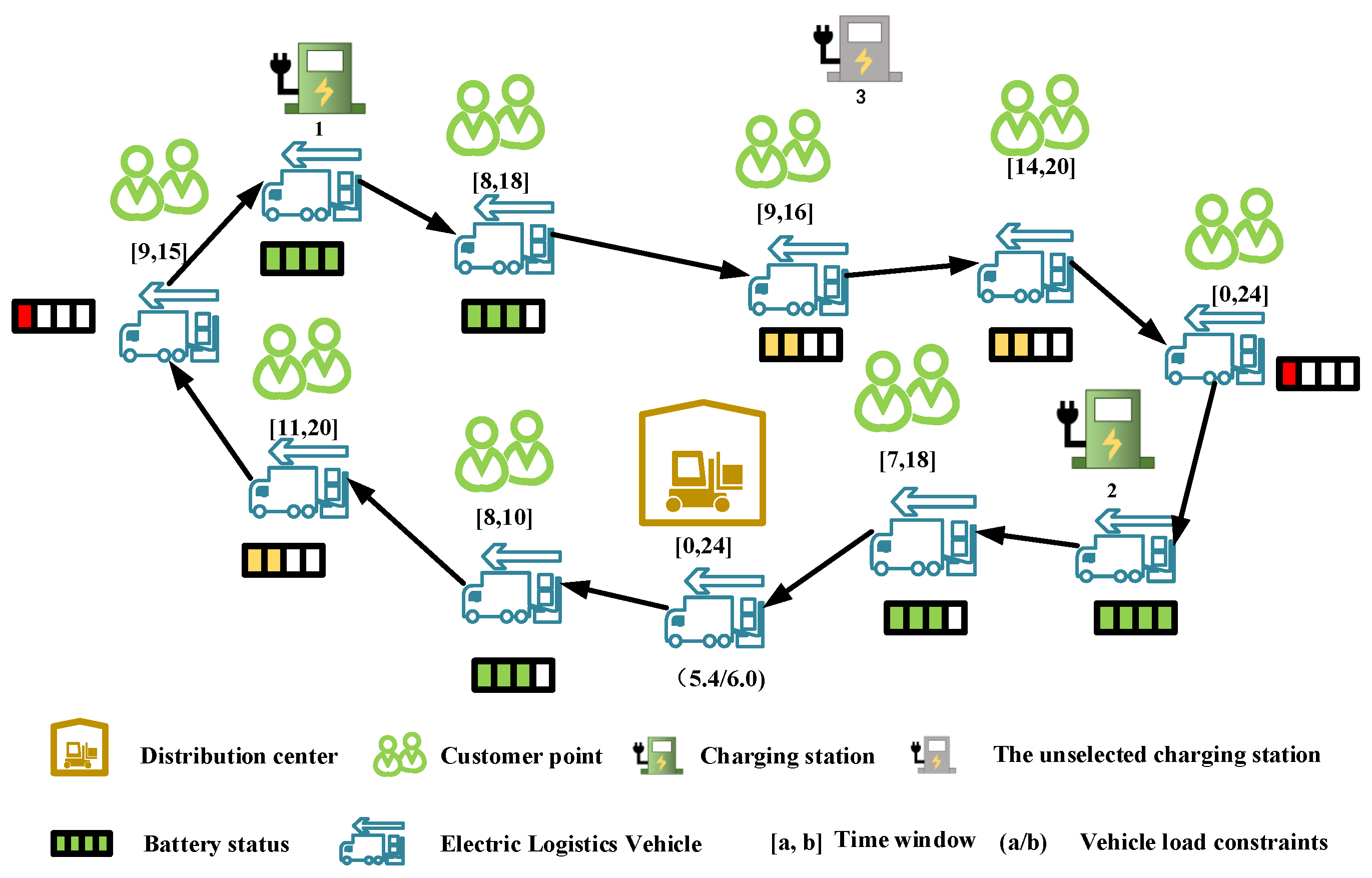
In solving the TW-LC problem using a genetic algorithm, chromosomes are coded in the form of integer coding. For example, if the number of customer points is 5, allowing for up to 3 logistics vehicles for service and 1 alternative charging station, then a feasible chromosome will be expressed as 12638475. The numbers 6 and 7 represent distribution centers, and 8 represents charging stations, dividing the customer points into 3 segments, i.e., into 3 paths. Path 1 is 0-1-2-0, path 2 is 0-3-8-4-0, and path 3 is 0-5-0. Let the number of customer points be N, the number of vehicles in use be K, and the number of charging stations be M. The length of the chromosome is N + K + M − 1, and the chromosome expression is (1, 2, 3, ……, N, N + 1, N + 2, ……, N + K + M − 1).

3.2. Path Construction Rules

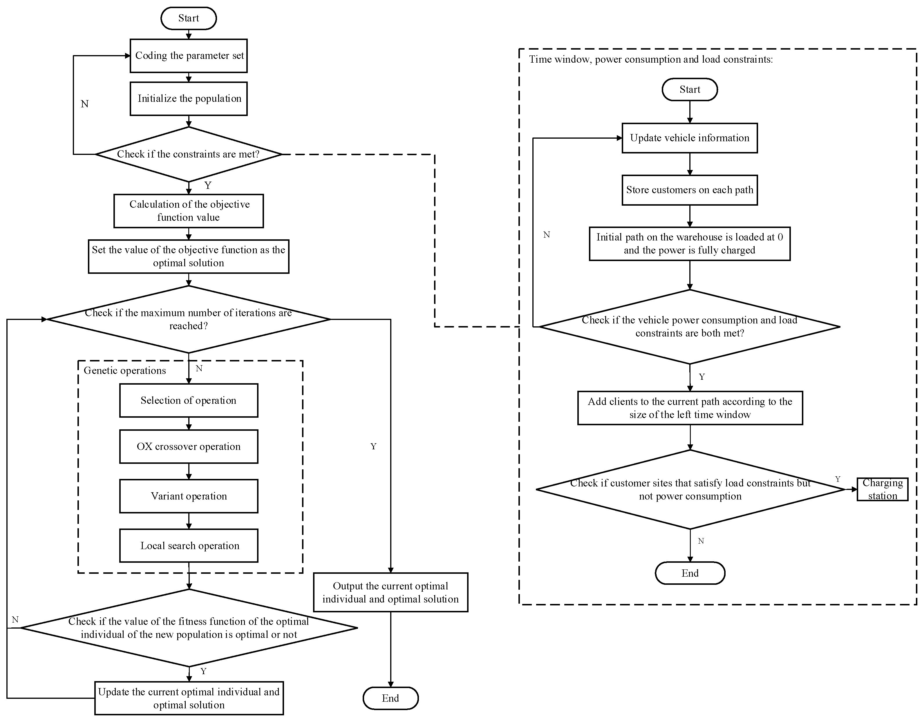
In the TW-LC problem, there are three cases of node locations, which are the distribution center, customer point, and charging station. The rules for path construction when the ELV passes through different nodes are as follows, and the flowchart is shown in Figure 2.

Step 1: Start the path construction: the starting point is the distribution center, the number of vehicles in use is initially set to 1, and the loading at the distribution center on the initial path is 0. According to the mileage-saving algorithm, search for the nearest customer point.

Step 2: If the current path is empty, add the customer point to the path directly. If there is only 1 customer point on the current path, check whether the customer point satisfies the load constraint; if so, add the customer point to the current path according to the left time window of the customer.

Step 3: Optimize the current path according to the farthest-insertion heuristic idea. If there are already n customer points on the path and n > 1, traverse the intermediate insertion position of n − 1 pairs of consecutive customer points and check whether the left time window of the newly inserted customer point can be between the left time windows of the customer points before and after the intermediate insertion position. If such an intermediate insertion position exists, then insert that client point into that position. If it does not, then that client point is added to the end of the current path. If the last client point is traversed, the path is updated, and the algorithm is skipped.

Step 4: In the path construction process, once the load constraint of the current vehicle is exceeded, first store the path driven by the previous vehicle; then, clear the original path and add a vehicle, with the starting point of the new vehicle being the distribution center.

Step 5: Site charging stations based on power constraints and construct charging stations at alternative locations until the penalty term of power in the path evaluation function is 0.

3.3. Introduction to Genetic Operators

3.3.1. Selection, Crossover, and Mutation Operations

The selection operation uses roulette selection to select a number of individuals with large fitness values for subsequent crossover, mutation, and localized scavenging operations [18]. The crossover operation of this algorithm uses an OX crossover to obtain two new sets of offspring by exchanging a portion of the gene positions of two sets of parents and removing duplicate genes. The mutation operation of this algorithm is performed by exchanging genes for two random positions of a set of parents to obtain a new set of offspring.

3.3.2. Local Search Operation

Local search is a heuristic algorithm for solving optimization problems and a type of greedy algorithm, which selects the best solution from the solution space of the domain of the current solution as the current solution for the next iteration each time until a locally optimal solution is reached. Starting from the local optimal solution, the domain of the current local optimal solution is searched; if there is a better solution, then the algorithm moves to it and continues to perform the search, and if not, then it stops and obtains the local optimal solution. The specific process is shown in Figure 3.

Since it is not easy to arrive at the optimal solution in a short time when solving complex problems, the addition of the local search operation can be the second-best solution to find a sub-optimal or near-optimal solution to the problem, which shortens the solution time of the algorithm, and adding the local search operation to the genetic algorithm can prevent it from falling into a local optimal situation [19]. Utilizing the idea of destruction and repair, a number of similar customer points on the current path are removed based on a similarity formula. The removed customer points are inserted back into the locations that minimize the increase in the total distance traveled by the vehicle as much as possible while satisfying the load constraints, time-window constraints, and power consumption constraints.

4. Arithmetic Testing and Example Applications

4.1. Simulation Environment

In this study, Solomon’s standard test algorithms were used for simulation. Six series were included to reflect the diversity of test cases. These were the C1, C2, R1, R2, RC1, and RC2 series. The C-series client point distribution is characterized by a cluster distribution, the R-series distribution is characterized by a uniform distribution, and the RC-series distribution is characterized by a mixture of the two distributions. The hardware CPU of the simulation computer was i7-10875, the memory was 32 GB, and the simulation software was Matlab2021a.

4.2. Small-Scale Simulation

The population size, iteration number, crossover probability, and mutation probability are the core parameters in the genetic algorithm, and the setting of these parameters will affect the performance of the algorithm. The above parameters should be set to the optimal value in order to obtain the optimal performance of the algorithm [20]. Therefore, before the start of the simulation, a small-scale simulation was carried out for the example of the R101 algorithm; the optimization of the relevant parameters was sought, and the following results were obtained.

From

Table 2. Simulation results for different population sizes and different iteration numbers.

Iteration Number = 200			Population Size = 200
Population Size	Optimal Path Length	Solution Time	Iteration Number	Optimal Path Length	Solution Time
100	1750.67	3.68 s	100	1871.55	4.79 s
150	1733.19	5.19 s	200	1733.85	8.29 s
200	1644.79	6.80 s	300	1624.32	12.84 s
250	1634.59	8.66 s	400	1619.27	16.98 s
300	1515.12	11.91 s	500	1533.60	21.36 s
350	1578.01	13.35 s	600	1590.88	26.05 s
400	1657.91	15.73 s	700	1658.84	30.53 s

and

Table 3. Simulation results for different crossover probabilities and different mutation probabilities.

Mutation Probability = 0.03			Crossover Probability = 0.7
Crossover Probability	Optimal Path Length	Solution Time	Mutation Probability	Optimal Path Length	Solution Time
0.4	1791.04	7.31 s	0.02	1810.15	7.93 s
0.5	1680.03	7.89 s	0.03	1752.73	8.50 s
0.6	1659.45	7.80 s	0.04	1627.77	8.37 s
0.7	1600.69	8.75 s	0.05	1541.54	8.39 s
0.8	1597.66	7.34 s	0.06	1579.11	8.18 s
0.9	1537.76	8.06 s	0.07	1564.11	7.88 s
1.0	1609.59	8.77 s	0.08	1564.32	7.90 s

, it can be seen that the objective function value is better when the population size is 500, the number of iterations is 500, the crossover probability is 0.9, and the mutation probability is 0.05. Therefore, in the subsequent simulation, the genetic algorithm parameters were set to the optimal values mentioned above.

4.3. Algorithm Stability Verification Analysis

The genetic algorithm designed in Section 3 was utilized to solve the model proposed in Section 2. In each set of algorithms, 50 points were randomly sampled as customer points. In addition to that, the node set contained one distribution center and four alternative charging stations, and up to five ELVs were available to provide distribution services. Each series of algorithms was run ten times to collect data such as the optimal path length, the number of constraint-violating paths, the number of charging stations selected, and the solution time. The results are shown in

Table 4. Statistics of test case results.

Arithmetic Series	Times	Optimal Path Length	Constraint Path Violations	Charging Stations Selected	Vehicles Utilized	Solution Time
C1 type	1	1660.32	0	2	5	30.85 s
	2	1590.12	0	2	5	30.37 s
	3	1641.78	0	2	5	31.52 s
	4	1760.42	0	1	5	29.23 s
	5	1690.63	0	2	5	30.88 s
	6	1783.19	0	3	4	29.97 s
	7	1702.62	0	2	5	29.82 s
	8	1502.03	0	4	4	29.17 s
	9	1658.25	0	2	5	29.96 s
	10	1533.93	0	2	5	28.91 s
Average		1652.33	0	2.2	4.8	30.04 s
C2 type	1	1601.52	0	2	5	30.53s
	2	1724.72	0	3	4	30.79 s
	3	1558.58	0	2	4	30.54 s
	4	1696.32	0	2	4	30.02 s
	5	1639.53	0	2	4	30.66 s
	6	1538.76	0	2	4	29.95 s
	7	1586.47	0	2	4	29.53 s
	8	1592.23	0	2	4	30.50 s
	9	1696.29	0	3	5	30.33 s
	10	1453.21	0	3	5	29.28 s
Average		1608.76	0	2.3	4.3	30.21 s
R1 type	1	1529.50	0	4	4	29.37 s
	2	1616.22	0	4	4	29.34 s
	3	1492.11	0	4	4	29.31 s
	4	1507.22	0	4	4	29.71 s
	5	1606.66	0	3	4	30.00 s
	6	1632.58	0	4	4	29.96 s
	7	1787.98	0	4	4	31.11 s
	8	1421.06	0	3	4	29.65 s
	9	1455.73	0	4	4	29.67 s
	10	1564.56	0	4	4	29.51 s
Average		1561.36	0	3.8	4.0	29.76 s
R2 type	1	1707.90	0	3	4	30.94 s
	2	1634.59	0	4	4	29.91 s
	3	1609.99	0	4	5	29.69 s
	4	1603.56	0	4	4	30.56 s
	5	1755.26	0	4	4	30.82 s
	6	1716.51	0	3	4	31.00 s
	7	1615.94	0	4	4	31.23 s
	8	1552.40	0	2	5	29.96 s
	9	1618.24	0	3	4	30.65 s
	10	1590.71	0	3	5	30.83 s
Average		1640.51	0	3.4	4.3	30.56 s
RC1 type	1	1953.73	0	4	5	32.53 s
	2	1921.72	0	4	4	33.64 s
	3	1981.98	0	4	4	32.71 s
	4	1843.53	0	3	4	34.09 s
	5	1814.36	0	4	4	32.51 s
	6	1998.31	0	4	4	33.33 s
	7	1983.63	0	3	4	33.39 s
	8	1846.56	0	3	4	32.28 s
	9	2066.77	0	3	4	34.51 s
	10	1905.16	0	2	5	32.73 s
Average		1931.58	0	3.4	4.2	33.17 s
RC2 type	1	1827.98	0	2	5	32.70 s
	2	1976.47	0	3	4	34.12 s
	3	1848.35	0	4	4	33.93 s
	4	1868.56	0	3	4	34.21 s
	5	1776.20	0	3	5	32.87 s
	6	1970.33	0	2	4	34.53 s
	7	1895.94	0	2	4	34.21 s
	8	1864.99	0	1	4	32.85 s
	9	1838.80	0	3	4	31.99 s
	10	1726.23	0	3	4	31.42 s
Average		1859.39	0	2.6	4.2	33.28 s

.

From Table 4, it can be seen that the number of constraint path violations is 0 after solving and iterating 500 times using the improved genetic algorithm for C-type, R-type, and RC-type algorithms, and it does not reach the maximum value with the number of charging stations selected and the number of vehicles used, so the present algorithm is effective in solving and optimizing the TW-LC problem.

4.4. Comparison between GA and IGA

In order to further verify the superiority of the proposed algorithm in this paper, this algorithm is compared with the traditional genetic algorithm with the same arithmetic cases. As can be seen from

Table 5. GA and IGA performance comparison.

Average	GA and IGA Performance Comparison
	GA	IGA	|(IGA − GA)/GA|%
Optimal path length	1931.15	1708.93	11.12%
Number of charging stations selected	3.85	2.95	22.97%
Number of vehicles in use	5.0	4.3	13.71%
Algorithmic complexity	58.60	31.17	46.81%

, the improved genetic algorithm shortens the optimal path by 11.12% on average; the number of charging stations selected and the number of vehicles used are reduced by 22.97% and 13.71%, respectively; and the complexity of the algorithm is reduced by 46.81% on average.

Figure 4 compares the objective function of the algorithms, i.e., the optimal path length. It can be seen that the improved genetic algorithm performs better in all kinds of arithmetic cases. In particular, the improvement is more obvious when dealing with the C-series arithmetic cases, whose distribution is characterized by clustering.

Figure 5 and Figure 6 compare the number of charging stations selected and the number of vehicles in use for the two algorithms. Selecting fewer charging stations and using fewer distribution vehicles under the same conditions will reduce the total cost of transportation. The improved genetic algorithm significantly improves the number of charging stations selected, even in more complex distribution examples such as the RC series, and it can significantly reduce the number of charging stations selected and increase the utilization rate of charging stations. In terms of the number of vehicles in use, the traditional genetic algorithm selects the maximum number of vehicles in all three series of examples, while the improved genetic algorithm, which incorporates the idea of the farthest-insertion heuristic into the algorithm, tries to rationally arrange and insert customer points into the path to maximize the reduction in the use of vehicles.

Figure 7 compares the algorithm complexity of the two algorithms. The traditional genetic algorithm easily falls into local optimal situations after iterating a certain number of times, which means that the objective function is not the global optimal value; at the same time, it also improves the complexity of the algorithm. As the improved genetic algorithm adds the idea of the local search, the method of destruction and repair is utilized in the solution, and the chromosome sequence of the optimal value is split and reorganized, which effectively prevents the algorithm from falling into the local optimal situation and shortens the solution time while improving the accuracy of the results.

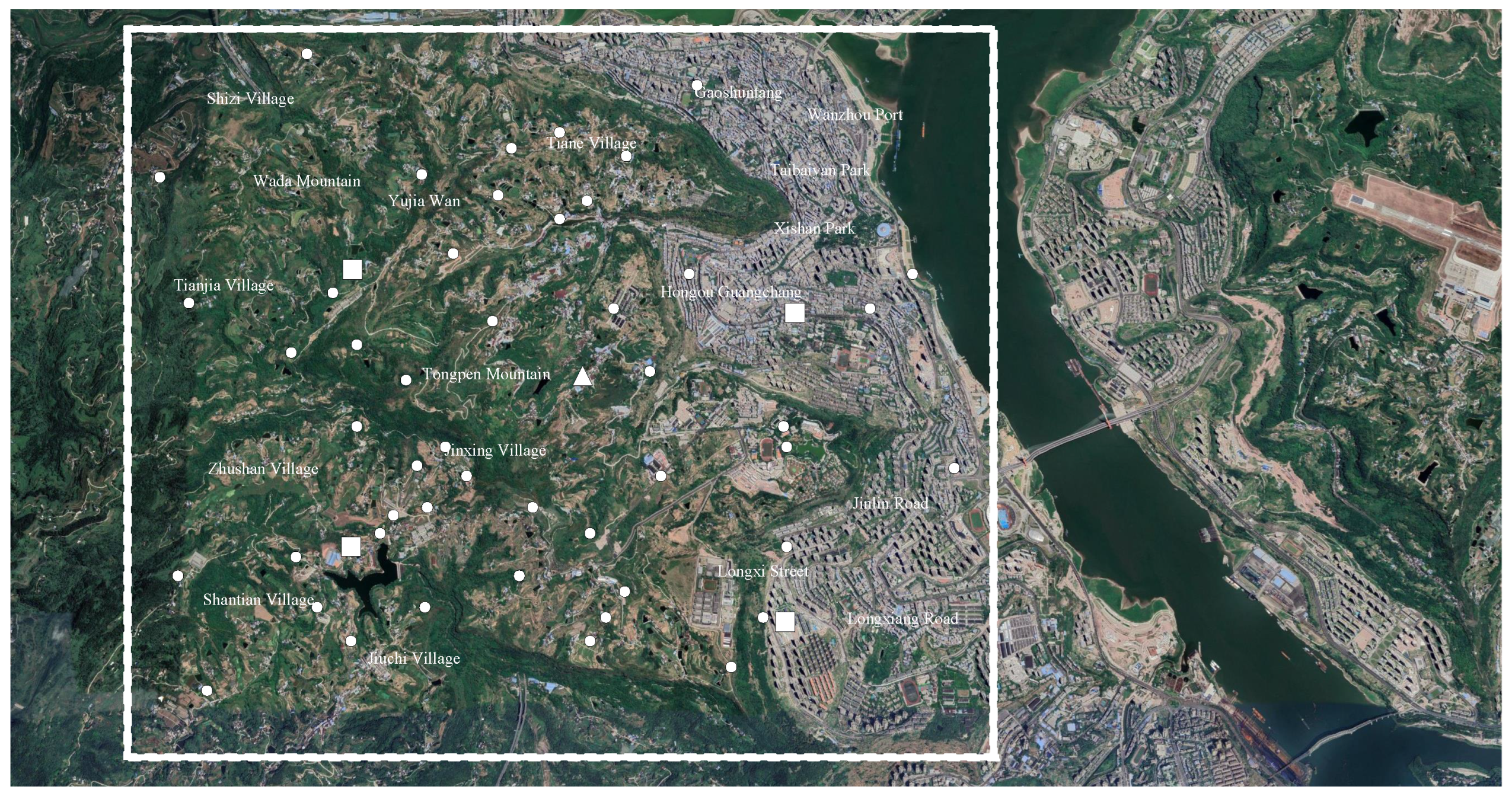
4.5. Analysis of Application Examples

In order to verify the reliability and practicality of the algorithm, a place in Chongqing, China, was selected for path planning and charging station location for the TW-LC problem in this area, with the optimal path as the objective function. A rectangular area with a range of 8 miles × 7 miles was selected, and 50 customer points, 4 locations of buildable charging stations, and 1 distribution center were used. The location information of each point was enlarged and transformed into a 2D Cartesian coordinate system at a ratio of 1:10. The schematic diagram of the nodes is shown in Figure 8, which was solved using the traditional genetic algorithm and the improved genetic algorithm; the solution results are shown in Figure 9, and the distribution scheme is shown in

Table 6. GA distribution program.

Path	Sequence
Path one	0 → 13 → 0
Path two	0 → 7 → 14 → 9 → 8 → 28 → 11 → 10 → 16 → 15 → 0
Path three	0 → 21 → 25 → 22 → 23 → 24 → 18 → 43 → 53 (recharge) → 17 → 2 → 27 → 20 → 29 → 51 (recharge) → 26 → 30 → 0
Path four	0 → 19 → 37 → 32 → 42 → 41 → 39 → 54 (recharge) → 35 → 46 → 36 → 34 → 38 → 40 → 33 → 31 → 44 → 45 → 0
Path five	0 → 47 → 4 → 1 → 5 → 12 → 3 → 48 → 49 → 52 (recharge) → 50 → 6 → 0

and

Table 7. IGA distribution program.

Path	Sequence
Path one	0 → 47 → 29 → 23 → 18 → 5 → 12 → 13 → 11 → 10 → 14 → 0
Path two	0 → 25 → 8 → 9 → 35 → 48 → 3 → 50 → 49 → 6 → 1 → 37 → 0
Path three	0 → 32 → 46 → 44 → 41 → 33 → 43 → 52 (recharge) → 42 → 36 → 2 → 31 → 39 → 34 → 40 → 4 → 45 → 38 → 0
Path four	0 → 21 → 17 → 7 → 26 → 19 → 51 (recharge) → 16 → 15 → 24 → 30 → 27 → 28 → 22 → 20 → 0

.

In this statistically optimal path, the traditional genetic algorithm selected a total of four charging stations and carried out four charging stops, and the optimal path length was 177.33 miles; the improved genetic algorithm selected two charging stations and carried out two charging stops in the middle of transportation, and the optimal path length was 154.17 miles. The number of charging stations selected decreased by 50%. In terms of vehicle use, the traditional genetic algorithm selected five paths and five vehicles to provide delivery service; the improved genetic algorithm selected four paths and four vehicles to provide service, and the number of vehicles selected decreased by 20%. And the improved genetic algorithm violated the time-window, load, and power consumption constraints 0 times, so this algorithm is reliable and advantageous in solving the TW-LC problem.

4.6. Analysis of Economic Indicators

In order to further analyze and compare the economic indicators of the model, the results of the example application above are used as an example. The unit electricity sales of the charging station operator and the annualized cost of the logistics company were calculated in terms of years, assuming that the logistics company carries out a delivery service once a day.

The unit electricity sales of the charging station operator is the amount of electricity sold per charging station $q_0$:

$$q_0=365\frac{OP·l_0}{n}$$

(16)

$l_0$ represents the power consumption per unit length of the ELV, which is set to 0.8 KWH/MILE; n represents the number of charging stations selected.

The logistics company’s one-year balance cost $C_0$ is the absolute value of the logistics company’s annualized total cost $C_1$ using the IGA minus the logistics company’s annualized total cost $C_2$ using the GA algorithm:

$$C_0=\left|C_1-C_2\right|$$

(17)

In the case of $C_1$, for example, the logistics company’s annualized total cost is

$$C_1=OP·l_0·e_p·365+n^{\prime }·U$$

(18)

$e_p$ denotes the unit price of electricity, which is set to 0.2 USD/KWH; $n^{\prime }$ denotes the number of vehicles utilized; and U denotes the unit vehicle purchase cost, which is set to USD 10,000.

The calculation results of specific economic indicators are shown in

Table 8. Analysis of economic indicators.

	Unit Electricity Sales/KWH	Total Annualized Cost/USD
GA	12,945.09	60,356.07
IGA	22,508.82	49,003.53

.

As shown in Table 8, the IGA improves the unit electricity sales by 73.88% and reduces the total annualized cost of the logistics company by 18.81% compared to the GA.

5. Conclusions

In this paper, we propose the TW-LC problem and design an improved genetic algorithm to solve the problem. Simulations were conducted using six different types of arithmetic examples and validated for a site in Chongqing, China, and the main conclusions are as follows.

The improved genetic algorithm optimizes the objective function compared with the traditional genetic algorithm, and the idea of the farthest-insertion heuristic reasonably arranges the sequence of all customer points, which shortens the optimal path by 11.12% on average; the improved genetic algorithm optimizes the transportation cost compared with the traditional genetic algorithm, which reduces the number of charging station selection and the number of vehicles used by 22.97% and 13.71% on average. In terms of economic metrics, compared to the GA, the IGA improved charging station unit sales by 73.88% and reduced the total annualized cost by 18.81%. It provides the decision makers of logistics companies with a lower-cost transportation solution for site selection; the improved genetic algorithm reduces the complexity by 46.81% compared with the traditional genetic algorithm, and the local search operation prevents the algorithm from falling into a local optimum and improves the algorithm’s computational efficiency.

The TW-LC problem is solved, but in order to reduce the complexity of the model, it does not take into account whether the vehicle supports the V2G mode, the amount of the load on the grid, and the co-existence of charging/exchange stations. In a future study of the TW-LC problem, we will continue to optimize the vehicle path, the number of charging stations selected, and the number of vehicles in use and further extend the model by accounting for whether or not the vehicle participates in grid interactions while charging and the co-existence of charging/exchange stations as constraints.