Study of Resistance Extraction Methods for Proton Exchange Membrane Fuel Cells Based on Static Resistance Correction

Abstract

Accurate extraction of polarization resistance is crucial in the application of proton exchange membrane fuel cells. It is generally assumed that the steady-state resistance obtained from the polarization curve model is equivalent to the AC impedance obtained from the electrochemical impedance spectroscopy (EIS) when the frequency approaches zero. However, due to the low-frequency stability and nonlinearity issues of the EIS method, this dynamic process leads to an additional rise in polarization resistance compared to the steady-state method. In this paper, a semi-empirical model and equivalent circuit models are developed to extract the steady-state and dynamic polarization resistances, respectively, while a static internal resistance correction method is proposed to represent the systematic error between the two. With the correction, the root mean square error of the steady-state resistance relative to the dynamic polarization resistance decreases from 26.12% to 7.42%, indicating that the weighted sum of the static internal resistance and the steady-state resistance can better correspond to the dynamic polarization resistance. The correction method can also simplify the EIS procedure by directly generating an estimate of the dynamic polarization resistance in the full current interval.

1. Introduction

In the face of increasingly complex environmental issues, traditional fossil energy sources, which lead to large amounts of greenhouse gas emissions, are no longer able to contribute to the healthy and sustainable development of the automotive industry [1]. As one of the key power alternatives to traditional energy supply devices, fuel cells have received attention for combining the advantages of internal combustion engines and traction batteries, including low pollution, high reliability, and long lifetimes [2].

A Proton Exchange Membrane Fuel Cell (PEMFC) adopts a polymer membrane that can conduct ions as electrolytes, so it is also known as a Polymer Electrolyte Fuel Cell (PEFC). A PEMFC is an electrochemical device that converts the chemical energy in the Hydrogen–Oxygen reaction directly into electrical energy. The reaction takes place at low temperatures, with water and heat as products. The conversion efficiency could be as high as 70% [3]. In addition, it has the advantages of high power-to-weight ratio and fast start-up speeds, so PEMFC is considered to be an ideal power source for fuel cell vehicles (FCVs) [4].

FCVs strive to secure a dominant position in the market for long-distance and heavy-duty transportation [5]. Presently, Europe is actively pursuing the development of a diverse array of hydrogen buses, and several hundred such units have already been deployed across numerous Chinese cities. According to the 2019 report by Market Research Future (MRFR), it is anticipated that the global market for automotive hydrogen and fuel cells will expand at a 25% CAGR until 2025 [6].

The promotion of FCVs requires investigating the external characteristics of PEMFC systems to solve control problems. It is necessary to properly determine the PEMFC characteristics in steady and dynamic modes [7]. Commonly used methods are mainly based on electrochemical impedance spectroscopy (EIS) and polarization curve tests, which are often used to obtain information about impedance, output voltage, and load current.

EIS, also known as AC impedance spectroscopy, which tracks the resistance to alternating currents in an electrochemical system, is useful for exploring the system’s frequency response. Currently, equivalent circuit models (ECMs), also known as electrical equivalent circuits, are the main technique for analyzing EIS data [8]. An ECM approximates the external properties of electrochemical reactions using a theoretical framework consisting solely of electrical components. Each component, including energy storage and dissipation elements, describes a physicochemical process within the system.

The polarization curve data reflects the polarization loss of the fuel cell stack, i.e., the degree of voltage deviation from the electrochemical theoretical electromotive force (EMF). The three polarization modes, including activation polarization, ohmic polarization, and concentration polarization, correspond to different types of polarization resistance in the electrochemical reaction, which can be measured, to some extent, using EIS. The various polarization resistances are components of the overall resistance of the PEMFC. Therefore, the extraction of the total internal resistance is the basis for the determination of the various loss mechanisms and their contribution ratios.

The most straightforward method of measuring internal resistance is the current cut-off method [9], which relies on the transient voltage and current after turning off the power supply to calculate the theoretical internal resistance. The double Kalman filter method estimates the impedance in real time by monitoring the voltage and current without disrupting the fuel cell stack’s normal functioning [10]. Most measurement algorithms require the construction of hypothetical ECMs based on empirical evidence [8].

Uncertainties in electrical components and circuit structures can cause ambiguities in interpreting EIS data using an ECM. Therefore, the construction of a reasonable ECM is a crucial research topic [8]. The Randles circuit, consisting of a solution resistance, double-layer capacitance, and charge transfer resistance, is a prevalent ECM [11] and serves as a foundation for other intricate ECMs.

Numerous studies have been conducted to propose solutions that analyze the sources of impedance in fuel cell stacks. Boillot et al. [12] studied the impact of gas pressure on polarization loss and concluded that a decrease in the hydrogen partial pressure leads to an increase in the high-frequency (HF) arc of the EIS data, while the low-frequency (LF) arc of the EIS decreases with an increase in the oxygen partial pressure.

Interpreting the mechanisms illustrated by EIS data often requires the derivation of the ECM from essential electrochemical and diffusion theories. Manzo et al. [13] introduced a standard circuit to depict the frequency response of cathode catalyst layers (CCLs) at diverse current densities. Choi et al. [14] analyzed the charge transfer resistance, mass transport resistance, high frequency resistance (HFR), and proton resistance in CCL, separating the components using a transmission-line model (TLM) and recursive method under different relative humidity conditions.

ECM methods can be ambiguous, as various circuit elements could potentially fulfill the fitting accuracy requirements of the acquired EIS data [15]. The distribution of the relaxation time (DRT) technique has recently received significant attention as a complementary approach to enhance the ECM analysis. DRT, as a model-free method, can identify the relaxation times of the electrochemical system by using the quasi-infinite series of R//C elements without considering the internal mechanism, with no prior knowledge being required.

Heinzmann et al. [16] explored the effect of varying partial pressures of hydrogen and oxygen on the polarization process, using the deconvolution approach to identify the characteristic peaks of the distribution function and confirming a significant level of cathodic polarization through comparison. Zhu et al. [17] conducted analyses of resistance components arising from the oxygen reduction reaction (ORR) in PEMFC. They developed a polarization curve model using kinetic parameters in line with theoretical formulas of the primary polarization sources. Furthermore, the DRT method was utilized to establish the inherent connection between the polarization curves and EIS. Finally, the steady-state resistance and DRT peaks were analyzed quantitatively to precisely determine the polarization process demonstrated by the DRT peaks.

Thosar et al. [18] captured the fundamental details of the physicochemical processes and derived an analytical equation for the polarization curve that is valid across the entire range of current densities. Using a physical model of the polarization curves, parameters with clear physical meaning can be obtained. Nevertheless, additional experiments in cyclic voltammetry and linear sweep voltammetry may be required [17]. Physical models have poor stability and often have issues meeting the requirements in terms of generalizability and operational accuracy. Consequently, empirical equations have been proposed to obtain correlations between fuel cell performance and various operational and geometrical parameters [19]. These empirical polarization equations typically share a similar mathematical form with physical equations [20].

Previous studies on methods for extracting resistance in fuel cells primarily concentrate on analyzing sources and accurately estimating individual internal resistance components, including charge transfer resistance, mass transport resistance, CCL proton resistance, etc. However, estimations of total polarization resistance with side-by-side comparisons between various measurement techniques are rarely undertaken. Some studies on quantitatively identifying polarization processes using EIS data necessitate not only the derivation of complicated physics and electrochemical formulae but also involve a challenging DRT-solving process. Changes in fuel cell stacks and operating conditions also make it difficult to find and summarize correspondences. However, in engineering applications, the PEMFC is frequently utilized as a black box to examine its control and diagnostic issues based on output characteristics. The adoption of a straightforward and effective resistance extraction method can greatly simplify calculations and experiments.

The rest of this paper is organized as follows: Section 2 describes the publicly available dataset used for validation in this paper; Section 3 derives steady-state resistance from a semi-empirical model of the polarization curve; Section 4 involves ECM-based dynamic polarization resistance extraction; and Section 5 involves the empirical static internal resistance weighting method, which completes the correction from the steady-state resistance to the dynamic polarization resistance; followed by conclusions in Section 6.

The novelty of this study is summarized as follows:

(1)

A method of extracting steady-state resistance is proposed, based on a semi-empirical model of polarization curves, to avoid the complexities of physical model calculation.

(2)

Based on the characteristics of the EIS data under different current density conditions, the corresponding ECMs are empirically constructed and the dynamic polarization resistance of the fuel cell stack is calculated accordingly.

(3)

A strategy to correct the steady-state resistance using static internal resistance weighting is suggested. This strategy is employed to explain the polarization resistance difference of a fuel cell stack from steady-state to dynamic processes.

2. Description of the Publicly Available Datasets Used for the Study

This study utilizes data solely from an open-source dataset, the IEEE PHM 2014 Data Challenge [21], provided by the FCLAB Research Federation. Experiments were carried out in test facilities that enable normal or accelerated ageing of PEMFC stacks under constant and variable operating conditions while controlling and gathering health monitoring data like power loads, temperatures, hydrogen and air stoichiometry rates, etc. Two identical fuel cell stacks, called FC1 and FC2, were both operated for more than 1000 h under different conditions, and the degradation of their output over time was monitored and recorded. In this paper, only the data from FC1 is used to extract the resistance, and it was operated under stationary conditions with the current density of 0.70 A/cm².

The FC1 is a 5-cell stack. Each cell has an active area of 100 cm². The experiments can provide not only voltage-time global historic curves but also intermittently perform static-dynamic characterization, each of which comprises a polarization curve test and EIS measurements that were conducted before and after it. The tests were carried out at eight different times ($t$ = 0, 48, 185, 348, 515, 658, 823, 991 h). In the polarization curve test, the stack and cells voltages were measured under a current ramp from 0 A/cm² to 1 A/cm² of 1000 s. The voltage of the PEMFC was measured to acquire the current-voltage curve in a steady-state through this method. Adjustment of the gas flow was carried out to keep stoichiometric factors constant.

Since the polarization curve test can modify the internal state of the fuel cell stack, thus modifying the EIS results, only the EIS data after the polarization curve test are used for analysis in this paper. EIS measurements have been made in the following order: Constant current of 0.70 A/cm², 0.45 A/cm² and 0.2 A/cm². Between every measure, a stabilization period of 15 min has been respected to guarantee the stability of parameters. The Nyquist plots of the complex impedance, at frequencies ranging from 50 mHz to 10 kHz, constitute the results of the EIS tests.

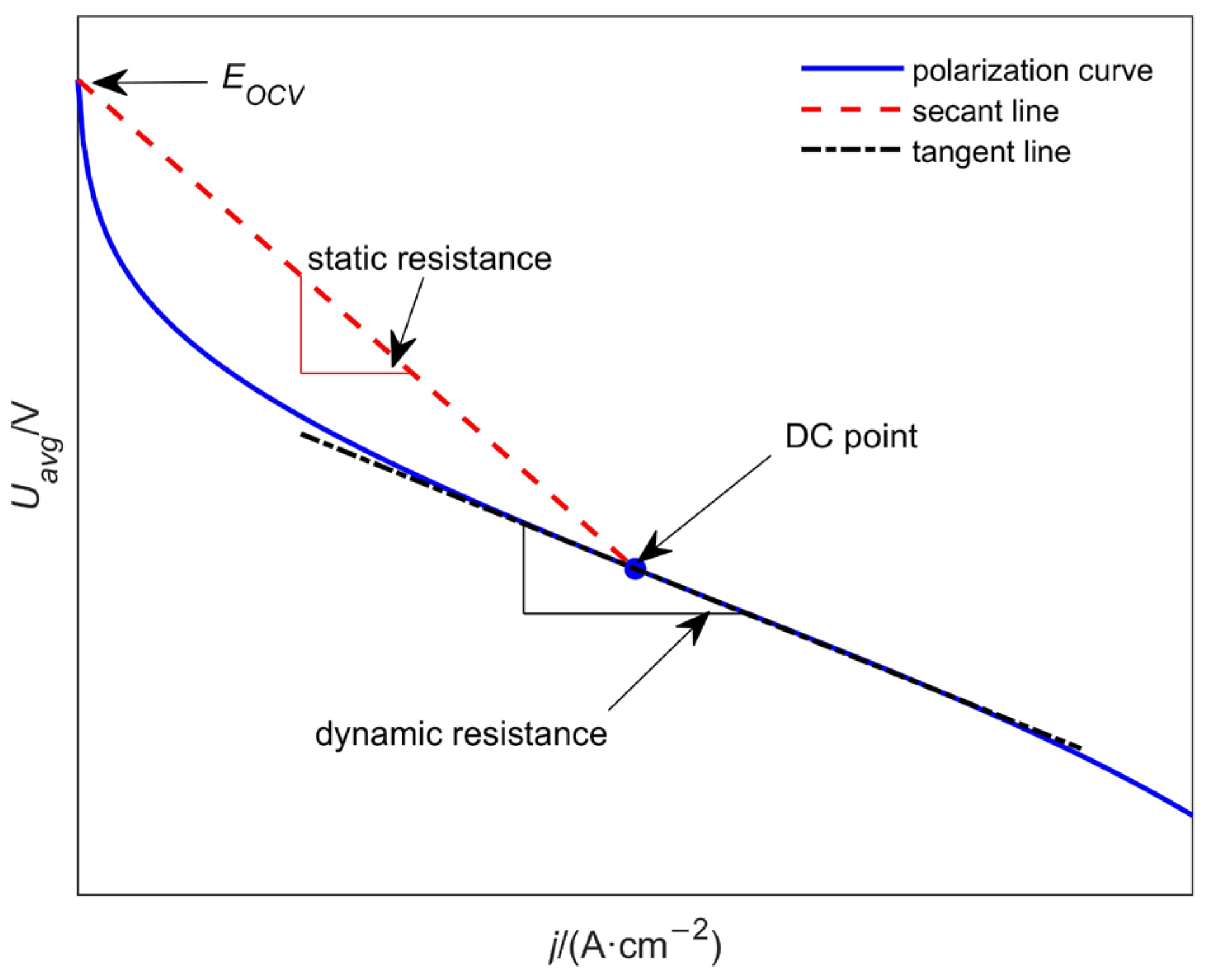
3. The Semi-Empirical Extraction Method for Dynamic and Static Internal Resistance

The polarization curves’ raw data for FC1 at each measurement time are presented in Figure 1, where $U_{\mathit{sum}}$ represents the FC1 output voltage and $j$ represents the current density.

Semi-empirical models of the polarization curve, as described by the Kim [22] and Fraser [23] models, can accurately represent the polarization loss of the output voltage in relation to the EMF. The Kim model is simple and practical, and it demonstrates high fitting accuracy for medium and high current density. However, the fitting accuracy is poor for open circuit voltage and small current densities. On the other hand, the Fraser model is highly applicable throughout the entire current interval. Nevertheless, it introduces operating temperatures and pressures that are not easily measured, consequently increasing the model’s complexity.

As a result of internal short-circuit currents and hydrogen crossover currents, to assess the voltage losses of the system, the external current of the fuel cell should be added to the internal loss currents. Consequently, Li et al. [24] suggested the following semi-empirical equation:

$$\begin{array}{c}U\left(j\right)=E_{\mathit{rev}}-b\times \lg \frac{j+j_{\mathit{loss}}}{j_{\mathit{loss}}}-R_{\mathit{ohm}}j-m{e}^{\mathit{nj}}\end{array}$$

(1)

In Equation (1), the input corresponds to the current density $j$, while the output represents the single-cell voltage $U$. Additionally, $E_{\mathit{rev}}$ denotes the reversible voltage, and $j_{loss}$ refers to the loss current density. The Tafel slope, represented by $b$, induces overvoltage due to the activation energy barrier in the logarithmic term. The resistance encountered by ions or electrons during conduction, following the Ohm’s law, corresponds to the linear term. The reaction rate is influenced by the slow diffusion of reactants, leading to additional overvoltage in the exponential term.

The mean voltage of a single cell $U_{avg}$ was recorded at each time with $j$ and used as the raw data for fitting, according to Equation (1). Results from fitting the polarization curve data for 48 h and 515 h are presented in Figure 2a,b, respectively. To assess the accuracy of the semi-empirical model, the root mean square error (RMSE) is utilized for quantitative analyses. This metric indicates the average deviation between the model’s estimates and the observed data, calculated as the square root of the expectation of the square of the difference between the two.

Let the number of raw data points at a specific time be $n$, the fitted voltage be $\widehat{U}\left(j\right)$, and the actual voltage be $U\left(j\right)$. The $\mathit{RMSE}$ is defined as in Equation (2), as follows:

$$\begin{array}{c}\mathit{RMSE}=\sqrt{\frac{1}{n}{\displaystyle \sum _j}{\left(\widehat{U}\left(j\right)-U\left(j\right)\right)}^2}\end{array}$$

(2)

Table 1. Polarization Curve Fitting Accuracy at Each Time.

$\mathrm{T}\mathrm{i}\mathrm{m}\mathrm{e}/\mathrm{h}$	$0$	$48$	$185$	$348$	$515$	$658$	$823$	$991$
$\mathit{RMSE}/\mathrm{m}\mathrm{V}$	$1.114$	$1.032$	$1.083$	$2.593$	$2.702$	$2.746$	$2.516$	$2.413$

indicates that each time has an $\mathit{RMSE}$ at a low level, allowing Equation (1) to characterize the polarization curve data effectively. In contrast to neural networks and physical models, the semi-empirical model avoids complex calculations and analyses while partially utilizing priori theories. It should be noted that the parameters from fitting semi-empirical formulae cannot be used to estimate actual physical parameters because of the interdependence of electrochemical mechanisms. For instance, directly using $E_{\mathit{rev}}$ and $R_{\mathit{ohm}}$ to estimate the reversible cell potential and ohmic resistance is considerably imprecise.

In the analysis of nonlinear components, there is a distinction between dynamic and static internal resistance. Static internal resistance pertains to the total internal resistance of the component at the DC point. When the battery produces a steady direct current of $I$, the terminal voltage is measured as $U$. Electromotive force of the battery is represented by $E_{\mathit{ocv}}$, and the static internal resistance at this point can be calculated using Equation (3), as follows:

$$\begin{array}{c} R_{\mathit{stat}}=\frac{E_{\mathit{ocv}} - U}{I}\end{array}$$

(3)

Since $E_{\mathit{ocv}}$ represents the open-circuit voltage of the PEMFC, it can be derived according to the semi-empirical Equation (1), as follows in Equation (4);

$$\begin{array}{c}{E}_{\mathit{ocv}}=U\left(0\right)=E_{\mathit{rev}}-m\end{array}$$

(4)

Dynamic resistance (AC resistance) evaluates the rate of change in voltage over current in a nonlinear element. Relying on the volt-ampere characteristic curve of the passive component, the dynamic resistance can be expressed as the slope of the curve at the static operating point. According to Equation (1), the negative slope of the tangent line of the polarization curve, $R_{\mathit{DC}}^{\prime }$, can be calculated using Equation (5), as follows:

$$\begin{array}{c}{R}_{\mathit{DC}}^{\prime }=-\frac{dU\left(i\right)}{di}=\frac{1}{\ln 10}\frac{b}{i + i_{\mathit{loss}}}+R_{el}+mn{e}^{ni}\end{array}$$

(5)

As shown in Figure 3, the negative slope $R_{\mathit{stat}}^{\prime }$ of the secant line joining the open-circuit voltage point and the DC operating point represents the static internal resistance, while the dynamic internal resistance $R_{\mathit{DC}}$ corresponds to the negative slope $R_{\mathit{DC}}^{\prime }$ of the tangent line at the static operating point. It should be noted that, when converting to PEMFC resistance (Ω), the negative slope of the straight line must consider both the active area and the number of cells to ensure a unified dimension.

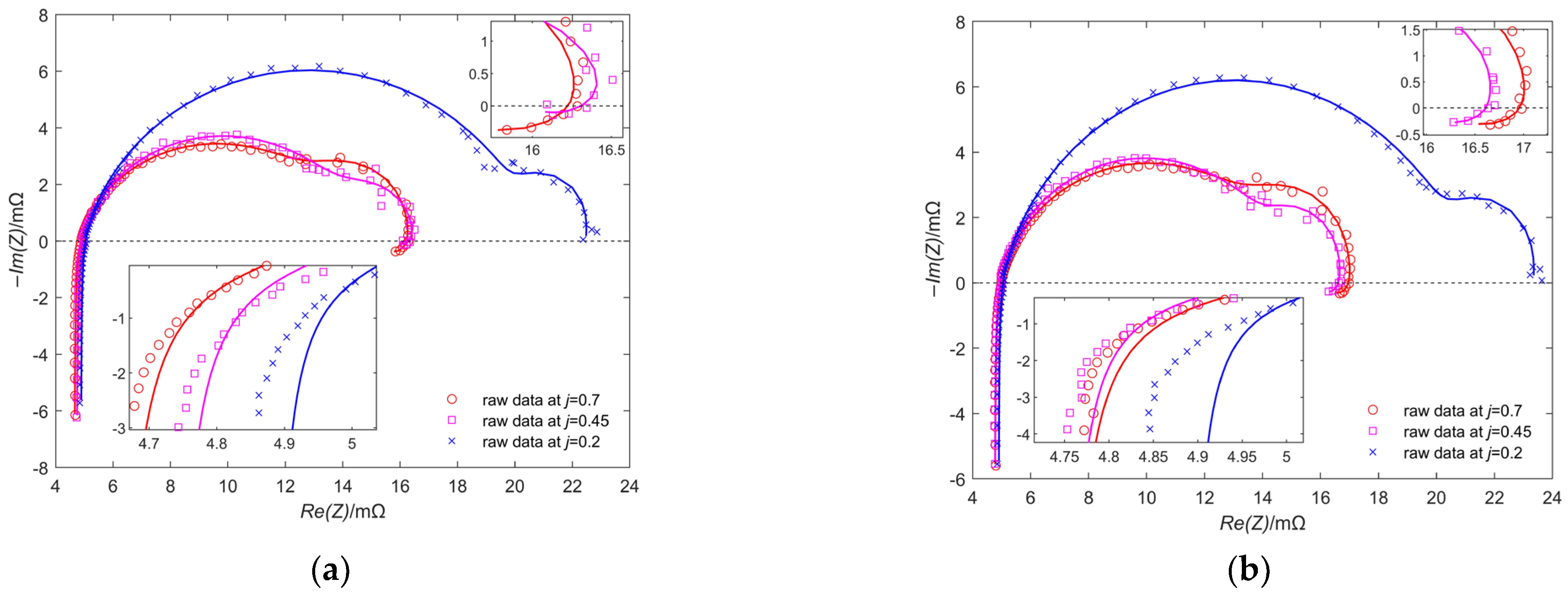
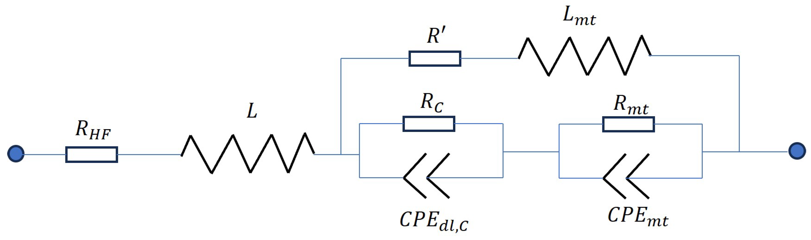
4. Dynamic Polarization Resistance Extraction Method Based on ECM

ECMs are typically constructed using empirical explanations of specific physical processes that appear within PEMFCs, which often necessitates limiting the circuit to a certain current range [13]. At each time, EIS tests were conducted under three different current densities, and the raw EIS data are depicted in Figure 4. The current densities illustrated in Figure 4a–c gradually decrease and thus possess somewhat distinct characteristics. The plots of the three sets share similarities, namely the presence of medium-frequency (MF) and LF semicircular arcs, as well as a HF inductive long tail. The EIS arc’s radius typically increases over time for each current density condition, excluding the two endpoints. This reflects a degradation phenomenon, as shown by an increase in resistance over time.

In the following, suitable components are selected to structure the ECM in order to precisely describe the different polarization processes of the PEMFC. Randles circuits are typically used to detail the electrochemical reactions at an electrode interface [25]. To better simulate anomalous diffusion caused by non-uniform electrodes, the double-layer capacitance may be substituted with a constant phase element (CPE) [26,27]. The CPE’s complex impedance can be expressed as follows:

$$\begin{array}{c}{Z}_{CPE}=\frac{1}{C{\left(i \cdot \omega \right)}^n}\end{array}$$

(6)

where $\omega$ is the angular frequency, C is the scale factor, $n$ is the CPE index characterizing the phase shift, and $i$ is an imaginary unit.

Owing to the sufficient supply of hydrogen, the hydrogen oxidation reaction (HOR) in the anode is ignored and only the impedances associated with ORR in the cathode and PEMFC main attachments are considered in this paper. The Randles element ($R_C//{CPE}_{dl,C}$), comprising of a charge transfer resistor in parallel with a CPE, is solely utilized to depict the ORR, which corresponds to the MF arc of the plots. The structure is serially connected with a feed line inductor L and a HFR $R_{HF}$. They correspond to the long tail at high frequency [28] and the HF real-axis extrapolation intercept [29], respectively. HFR is typically used to denote the ohmic internal resistance that characterizes the total conductance of protons and electrons [30]. However, certain studies [17] have demonstrated that the HFR corresponds to only the non-electrode components of the ohmic internal resistance, specifically the proton transport resistance of the membrane, interface contact resistance, and electron transport resistance of the gas diffusion layer (GDL), CCL, and channels. The ohmic internal resistance’s electrode component corresponds to a DRT peak, which is attributed to the CCL ionomer’s proton transport resistance.

The reactant transport limitations in the CCL electrolyte were not considered in the above analyses [13]. To be applicable to higher current densities, the following corrections are required. The $R_{mt}//{CPE}_{mt}$ element is connected in series, which corresponds to the mass transfer constraint due to oxygen diffusion in the CCL (LF capacitive arc) [30]. At ultra-low frequencies, the small arc with a positive imaginary part causes the curve to bend towards a smaller real part. This phenomenon corresponds to mass transfer processes under a state of water flooding [31], carbon monoxide poisoning, or adsorbed species in the CCL [13], as discussed in detail in Section 5.3. This feature can generally be characterized by connecting an inductor $L_{mt}$ in parallel with the LF element ($R_{mt}//{CPE}_{mt}//L_{mt}$). In contrast to the general structure, Kim et al. [32] achieved a highly accurate prediction of the state of health (SOH) by adding inductive branching ($L_{mt}\perp R\prime$) to the LF and MF components.

In summary, for the two higher current density cases of $j$ = 0.7, 0.45 A/cm², the ECM is built in accordance with Figure 5. For the low current density condition of $j$ = 0.2 A/cm², the relevant ECM is detailed in Figure 6. This is due to the ultra-LF inductive effect being absent in Figure 4c, leading to the correction structure being removed to guarantee the precision.

The parameters of the constructed ECM can be determined by a complex nonlinear least-squares fit (CNLS) approximation [11]. In Figure 7, (a) and (b) represent the fitting results for 185 h and 658 h, respectively. It can be observed that the EIS plots for current densities of 0.7 and 0.45 A/cm² are comparable but differ from the plots for a current density of 0.2 A/cm². Therefore, the use of the ECMs depicted in Figure 5 and Figure 6 is appropriate.

The accurate fit within the ultra-LF inductive area, presented in the upper right corner of Figure 7a,b, confirms the precision of the ECMs displayed in Figure 5. In the HF inductive region, which is shown in the lower left corner, there are minor deviations observed for each current density condition. These deviations could be due to the omission of the HOR in all the above ECMs.

For an assessment of the fitting accuracy to the EIS data, the Euclidean distance between the fitted result and the raw data points in the complex plane can be used. Let the EIS measurements with current density $j$ and time $t$ be $Z_{j,t}$, and the fitting result be ${\widehat{Z}}_{j,t}$. The mean square value of the Euclidean distance between them is shown in Equation (7), as follows:

$$\begin{array}{c}{\mathit{err}}_{j,t}=\frac{1}{n_f}{\displaystyle \sum _f}\left[{\left(Re Z_{j,t}\left(f\right)-Re {\widehat{Z}}_{j,t}\left(f\right)\right)}^2+{\left(Im Z_{j,t}\left(f\right)-Im {\widehat{Z}}_{j,t}\left(f\right)\right)}^2\right]\end{array}$$

(7)

In Equation (7), ${\widehat{Z}}_{j,t}$ and $Z_{j,t}$ are functions of the frequency $f$ (where $f=\omega /2\pi$). $Re Z$ and $Im Z$ denote the real and imaginary components of the complex impedance $Z$, respectively. In addition, $n_f$ represents the number of EIS data points used. The average of all ${\mathit{err}}_{j,t}$ values under a specific current density condition is calculated and converted to the resistance dimension, as shown in the following Equation (8):

$$\begin{array}{c}{\mathit{score}}_j=\sqrt{\frac{1}{n_t}{\displaystyle \sum _t}{\mathit{err}}_{j,t}}\end{array}$$

(8)

The CNLS fitting accuracies are all high for the EIS data under each current density conditions. The scores are of the same order of magnitude, as

Table 2. Fitting Accuracy of EIS Data for Each Current Density Condition.

$j/\mathrm{A} \mathrm{c}{\mathrm{m}}^{-2}$	$0.7$	$0.45$	$0.2$
$\mathit{score}/\mathrm{m}\mathsf{\Omega }$	$9.69\times {10}^{-2}$	$0.175$	$0.171$

illustrates. This finding demonstrates that the ECMs constructed separately for EIS data at different current densities are effective.

During EIS examinations, the electrode system located at the static operating point is perturbed by small amplitude sinusoidal currents or voltage signals at different frequencies. The aim is to evaluate the response signal of the system to ascertain the dynamic impedance of the fuel cell stack. The dynamic polarization resistance $R_{\mathit{EIS}}$ can characterize the dynamic process, which is obtained by extrapolating from the EIS data under the condition of $f$→0, as shown in the following Equation (9):

$$\begin{array}{c}{R}_{\mathit{EIS}}=\underset{f\to 0}{\lim }Z\left(f\right)\end{array}$$

(9)

The zero-frequency impedance can be calculated from the circuit structure once the appropriate ECM has been constructed from the EIS data. The results for medium and high current densities can be determined from Figure 5. Additionally, the dynamic polarization resistance for $j$ = 0.45 and 0.7 A/cm² is shown in Equation (10), as follows:

$$\begin{array}{c}{R}_{\mathit{EIS}}=R_{HF}+\frac{\left(R_C + R_{\mathit{mt}}\right)R^{\prime }}{R_C + R_{mt} + R^{\prime }}\end{array}$$

(10)

For the low current density condition of $j$ = 0.2 A/cm², the zero-frequency impedance of the ECM is shown in Equation (11) from Figure 6.

$$\begin{array}{c}{R}_{\mathit{EIS}}=R_{HF}+R_C+R_{mt}\end{array}$$

(11)

5. Resistance Extraction Results and Discussion

5.1. Relationship between Dynamic and Steady-State Polarization Resistances

The polarization curve test determines the stationary current−voltage pattern of the fuel cell stack and reflects the steady-state behavior of the PEMFC. The polarization resistance attained from the steady process is denominated as the steady-state resistance. As the polarization curve test can be viewed as the EIS test, with AC excitation at frequency $f$ = 0, it is treated as a specific scenario of the latter, where frequency tends towards 0. In summary, as shown in Equation (12), the steady-state resistance $R_{\mathit{DC}}$, derived from the negative slope of the tangent line of the polarization curve, is theoretically equivalent to the dynamic polarization resistance $R_{\mathit{EIS}}$ obtained from the EIS test conducted under the condition $f$→0 [33].

$$\begin{array}{c}{R}_{\mathit{EIS}}=\underset{f\to 0}{\lim }Z\left(f\right)=R_{\mathit{DC}}\end{array}$$

(12)

The correspondence in theory between the $R_{\mathit{DC}}$ and the $R_{\mathit{EIS}}$ could be attributed to the fact that EIS, as a quasi-stationary frequency domain measurement technique [8], is compatible with static methods like polarization curve tests. Since the excitation signal applies alternating, minor cathodic and anodic processes on the system that do not result in cumulative changes to the electrode state even over long periods of time, the electrochemical system in the EIS examination can be deemed as linear around its DC operating point. Calculating the AC impedance of such a linear system at frequencies close to 0, its ohmic components can then be approximated by the slope of the volt-ampere characteristic curve at the DC point.

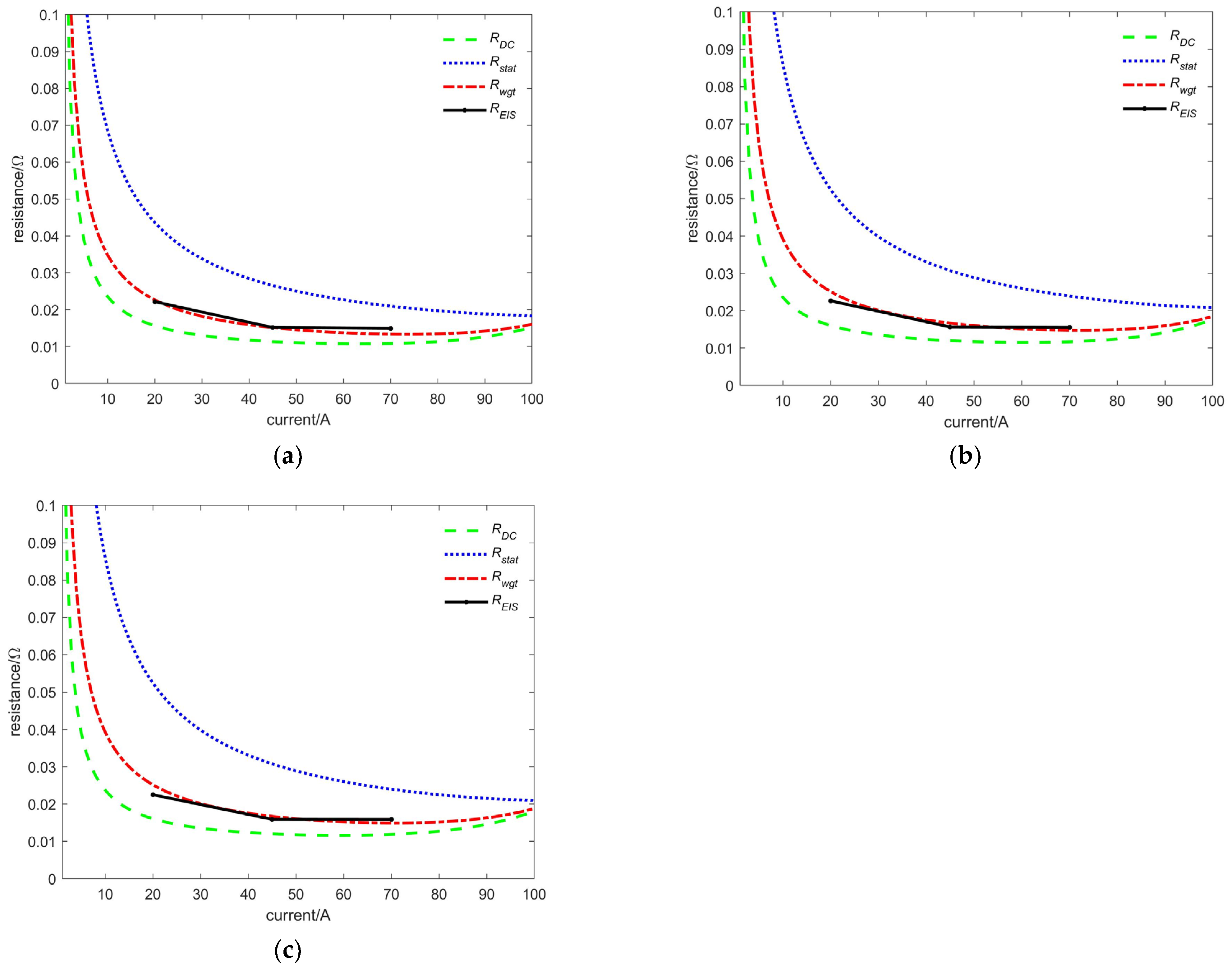
5.2. Static Internal Resistance Correction Method

Figure 8 shows the extraction results of the resistances, where (a), (b), and (c) correspond to the resistance-current curves at 0 h, 348 h, and 515 h, respectively. It has been observed that the dynamic polarization resistance $R_{\mathit{EIS}}$ is greater than the steady-state polarization resistance $R_{\mathit{DC}}$ and less than the static internal resistance $R_{\mathit{stat}}$ under a given current condition. In fact, the extracted resistance data for all eight times share this characteristic. Unlike the relationship demonstrated in Section 5.1, the $R_{\mathit{EIS}}$ in Figure 8 consistently exhibits a certain systematic error above the $R_{\mathit{DC}}$ at any time and current density condition. This systematic error is limited to approximately 7 mΩ.

Chatenet et al. [34] outlined principles that should be adhered to when realizing EIS, one of which is the need for measurements to demonstrate linearity and stability. The Kramers−Kronig transforms can be used to verify the above requirements, but this obviously does not eliminate the nonlinearities and instabilities in the quasi-stationary measurement approach. For imperfect EIS data, a method is proposed to approximate the zero-frequency impedance of the ECM using a weighted summation of the dynamic and static internal resistance, as in Equation (13), as follows:

$$\begin{array}{c}{R}_{\mathit{wgt}}=75\%R_{\mathit{DC}}+25\%R_{\mathit{stat}}\end{array}$$

(13)

This method is essentially a correction of $R_{\mathit{DC}}$ using $R_{\mathit{stat}}$. For the purpose of comparison, Figure 8 also includes the curves of the correction result $R_{\mathit{wgt}}$ with the current at specific times.

As demonstrated in Figure 8, the $R_{\mathit{stat}}$ decreases consistently with the increase in current and the rate of change declines gradually. This suggests that the total internal resistance also drops progressively with the current hike. $R_{\mathit{DC}}$, on the other hand, exhibits a concave function pattern that is low in the middle and high on both sides, and the minimal value point is situated near the medium current density of 0.6 A/cm². In the medium current density region, only the ohmic polarization requires consideration; however, in the low and high current density regions, the effects of activation polarization and concentration polarization need to be considered, respectively. As voltage data was not measured for higher current densities, growth in $R_{\mathit{DC}}$ was reduced in this region due to concentration polarization. Therefore, no growth occurred in the high current density region when calculating the total internal resistance, $R_{\mathit{stat}}$.

As depicted in Figure 8, the correction result $R_{\mathit{wgt}}$ is markedly comparable to $R_{\mathit{EIS}}$ and sits between $R_{\mathit{DC}}$ and $R_{\mathit{stat}}$ curves. To assess the relative deviation of EIS measurements from the polarization curve measurements before and after applying the weighted correction, the $\mathit{RMSE}$ is constructed as a metric. In Equations (14) and (15), $R_{\mathit{DC}}$ and $R_{\mathit{wgt}}$ are resistances at the relevant time and current density.

$$\begin{array}{c}{\mathit{RMSE}}_{\mathit{DC}}=\sqrt{\frac{1}{n_t + n_j}{\displaystyle \sum _t^{n_t}}{\displaystyle \sum _j^{n_j}}{\left(\frac{R_{\mathit{EIS}} - R_{\mathit{DC}}}{R_{\mathit{EIS}}}\right)}^2}\end{array}$$

(14)

$$\begin{array}{c}{\mathit{RMSE}}_{\mathit{wgt}}=\sqrt{\frac{1}{n_t + n_j}{\displaystyle \sum _t^{n_t}}{\displaystyle \sum _j^{n_j}}{\left(\frac{R_{\mathit{EIS}} - R_{\mathit{wgt}}}{R_{\mathit{EIS}}}\right)}^2}\end{array}$$

(15)

Furthermore, the total number of time nodes $n_t$ = 8 and the total number of current densities $n_j$ = 3. The results of the calculations for the $\mathit{RMSE}$ are presented in

Table 3. Relative Error before and after Weighted Correction.

${\mathit{RMSE}}_{\mathit{DC}}$	${\mathit{RMSE}}_{\mathit{wgt}}$
$26.12\%$	$7.42\%$

.

Table 3 demonstrates that the steady-state resistances achieved from the polarization curve model have an average reduction of 26.12% in comparison to the ECM zero-frequency resistances for all time and current density conditions. The relative error of more than a quarter is clearly not explained by random disturbances in the test process, which will be analyzed in Section 5.3 based on specific phenomena in the EIS data.

After correction, the ${\mathit{RMSE}}_{\mathit{wgt}}$ decreased to 7.42%. This suggests that the adjusted outcome $R_{\mathit{wgt}}$ of the $R_{\mathit{DC}}$ can more accurately approximate the dynamic polarization resistance $R_{\mathit{EIS}}$ in any time or current density situation. This result is displayed in Figure 8, where $R_{\mathit{EIS}}$ and $R_{\mathit{wgt}}$ exhibit almost equal values.

5.3. Analysis and Discussion

As illustrated in Figure 4a,b, under medium to high current density conditions, the EIS data, in the ultra-low frequency range (typically below 0.22 Hz), crosses the real axis and displays a pseudo-inductive behavior. This behavior can be explained by two common factors: side-reaction of intermediate species and water transport [35,36]. The water transport and side-reaction resistance, $R_w$, is often used to represent this phenomenon.

The analysis of pseudo-inductive behavior was conducted through the DRT method discussed in [17]. To ensure high-quality EIS data for DRT, it is necessary to remove the inductive information that is unrelated to the capacitive-dependent dynamics. This can be accomplished by truncating HF and ultra-LF inductive data without significantly affecting the accuracy of subsequent DRT fitting. Using the DRT algorithm, which excludes inductive effects, it is evident that the $R_{\mathit{DC}}$ acquired from the steady process is lower than the low frequency intercept of the DRT fit across all current densities. The difference between the actual and fitted LF intercepts correlates with the PEMFC’s resistance reduction (voltage recovery) processing from a dynamic to steady-state. It should be noted that the difference $R_w$ shares an eigenpeak with the mass transfer process in the DRT, thus posing a challenge to differentiation.

This research adopts the ECM method, which considers the pseudo-inductive behavior at ultra-low frequencies and the feed line inductor at high frequencies, in contrast to the above DRT method. Nonetheless, there is still a systematic error between $R_{\mathit{EIS}}$ derived from the ECM and steady-state resistance $R_{\mathit{DC}}$. This could potentially be attributed to the inadequate ultra-low frequency range of 0.05 Hz, which fails to capture the entirety of the pseudo-inductive arc. As obtaining the complete arc at ultra-low frequencies through EIS measurements is impractical due to the time consumption and poor stability and nonlinearity issues [35], the ECM utilized in this paper provides a more viable solution. Section 4 analysis shows that the ECM has a high fitting accuracy across the entire frequency measurement range, with Figure 7 illustrating that its fitting curve at ultra-low frequency aligns with the original data trend. A similar ECM can be used to achieve high-accuracy predictions of PEMFC performances, as demonstrated by a related study [32].

In this paper, the dynamic polarization resistance $R_{\mathit{EIS}}$ was higher than the steady-state resistance $R_{\mathit{DC}}$ when creating the ECM, despite considering the influence of inductive effects. This systematic error could be attributed to insufficient linearity at the static operating point in the quasi-stationary method, and it could therefore fluctuate based on the EIS test’s disturbance amplitude and the fuel cell stack’s intrinsic characteristics. The procedure outlined in Section 5.2 utilizes weighted values of the dynamic and static internal resistance of the PEMFC to estimate the polarization resistance obtained from quasi-stationary measurements. As presented in Equation (13), the static internal resistance $R_{\mathit{stat}}$ is used to affect a weighted correction to the dynamic internal resistance $R_{\mathit{DC}}$, with the weight ratio of them remaining constant at 1:3. It is important to note that this is an empirical constant, which may change with alterations to the fuel cell stack and its testing conditions.

The average relative difference between the corrected steady-state resistance and the ECM zero-frequency resistance decreased from 26.12% to 7.42%. Therefore, the $R_{\mathit{DC}}$ extracted from the polarization curve model, corrected by $R_{\mathit{stat}}$, can establish a precise match with $R_{\mathit{EIS}}$. The effectiveness of this correction method may be attributed to the inclusion of the static internal resistance component, enforcing a correction based on the static operating point of the fuel cell stack, as well as the characteristics of the polarization phenomenon.

The function of PEMFCs is frequently subjected to disturbances comparable to those encountered in EIS experiments. However, the EIS has limitations in regard to achieving high-precision measurements, as it can only measure under specific current density conditions. By employing the resistance extraction method, a corrected resistance-current continuous curve can be developed based on the polarization curve data. This leads to precise estimation of the zero-frequency resistance obtained from EIS measurements over the full current interval. The polarization resistance obtained by extraction can be used not only for catalyst selection [37] and evaluation of assembly pressure [38], but also for indicating the humidity of the proton exchange membrane [10].

6. Conclusions

In this paper, based on the IEEE test data, the steady-state polarization resistance is extracted using a semi-empirical model of the polarization curve while the dynamic polarization resistance is extracted using an ECM that accounts for inductive effects, with a large systematic error being discovered between them. A correction method based on the weighting of the static internal resistance is then proposed to unify the steady-state and dynamic polarization resistances. This resistance extraction method, which can rely directly on the polarization curve data to extract the dynamic polarization resistance, helps to simplify the test process and is of great importance for the study and diagnosis of the external characteristics of fuel cell stacks. The following conclusions were drawn:

• Based on the semi-empirical model of the polarization curves, it is possible to obtain the steady-state polarization resistance $R_{\mathit{DC}}$ and the static internal resistance $R_{\mathit{stat}}$ of fuel cell stacks with high accuracy, avoiding the complicated calculation process of physical models.
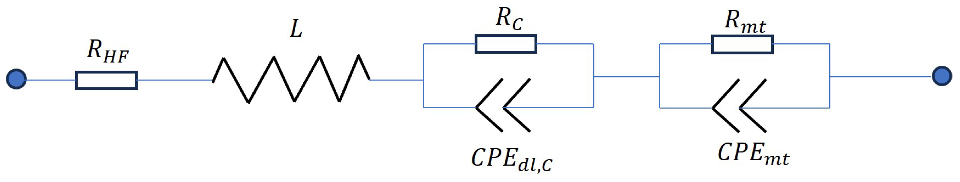
• By considering the pseudo-inductive effect at ultra-low frequencies and the feed line inductor at high frequencies, it is feasible to design ECMs that align with various current density conditions based on the characteristics of the EIS data. From these ECMs, the dynamic polarization resistance $R_{\mathit{EIS}}$ can be extracted.
• Estimating the zero-frequency resistance using $R_{\mathit{DC}}$ leads to a considerable systematic error. The use of an $R_{\mathit{DC}}$ correction strategy based on $R_{\mathit{stat}}$ weighting can markedly decrease the relative error between steady-state and dynamic polarization resistance. The empirical weights utilized could differ depending on the perturbation amplitude of the EIS test and the intrinsic characteristics of the fuel cell stack.

References

1. Park, J.; Oh, H.; Ha, T.; Lee, Y.I.; Min, K. A review of the gas diffusion layer in proton exchange membrane fuel cells: Durability and degradation. Appl. Energy 2015, 155, 866–880. [Google Scholar] [CrossRef]
2. Mert, S.O.; Dincer, I.; Ozcelik, Z. Performance investigation of a transportation PEM fuel cell system. Int. J. Hydrogen Energy 2011, 37, 623–633. [Google Scholar] [CrossRef]
3. Demuren, A.; Edwards, R.L. Modeling Proton Exchange Membrane Fuel Cells—A Review. In 50 Years of CFD in Engineering Sciences; Springer: Singapore, 2020. [Google Scholar]
4. Bernay, C.; Marchand, M.; Cassir, M. Prospects of different fuel cell technologies for vehicle application. J. Power Sources 2002, 108, 139–152. [Google Scholar] [CrossRef]
5. Olabi, A.G.; Wilberforce, T.; Abdelkareem, M.A. Fuel cell application in the automotive industry and future perspective. Energy 2021, 214, 118955. [Google Scholar] [CrossRef]
6. Market Research Future®. Part of WantStats Research and Media Pvt. ‘Hydrogen and Fuel Cells Market Research Report—Forecast to 2025’ ID: MRFR/E&P/4491-CR. May 2018. Available online: https://www.marketresearchfuture.com/reports/hydrogen-fuel-cells-market-5947 (accessed on 1 February 2024).
7. Loskutov, A.; Kurkin, A.; Shalukho, A.; Lipuzhin, I.; Bedretdinov, R. Investigation of PEM Fuel Cell Characteristics in Steady and Dynamic Operation Modes. Energies 2022, 15, 6863. [Google Scholar] [CrossRef]
8. Tang, Z.; Huang, Q.-A.; Wang, Y.-J.; Zhang, F.; Li, W.; Li, A.; Zhang, L.; Zhang, J. Recent progress in the use of electrochemical impedance spectroscopy for the measurement, monitoring, diagnosis and optimization of proton exchange membrane fuel cell performance. J. Power Sources 2020, 468, 228361. [Google Scholar] [CrossRef]
9. Reggiani, U.; Sandrolini, L.; Burbui, G.L.G. Modelling a PEM fuel cell stack with a nonlinear equivalent circuit. J. Power Sources 2007, 165, 224–231. [Google Scholar] [CrossRef]
10. Wei, Y.; Zhao, Y.; Yun, H. Estimating PEMFC ohmic internal impedance based on indirect measurements. Energy Sci. Eng. 2021, 9, 1134–1147. [Google Scholar] [CrossRef]
11. Danzer, M.A.; Hofer, E.P. Analysis of the electrochemical behaviour of polymer electrolyte fuel cells using simple impedance models. J. Power Sources 2009, 190, 25–33. [Google Scholar] [CrossRef]
12. Boillot, M.; Bonnet, C.; Jatroudakis, N.; Carre, P.; Didierjean, S.; Lapicque, F. Effect of Gas Dilution on PEM Fuel Cell Performance and Impedance Response. Fuel Cells 2006, 6, 31–37. [Google Scholar] [CrossRef]
13. Cruz-Manzo, S.; Chen, R. A generic electrical circuit for performance analysis of the fuel cell cathode catalyst layer through electrochemical impedance spectroscopy. J. Electroanal. Chem. 2013, 694, 45–55. [Google Scholar] [CrossRef]
14. Choi, J.; Sim, J.; Oh, H.; Min, K. Resistance Separation of Polymer Electrolyte Membrane Fuel Cell by Polarization Curve and Electrochemical Impedance Spectroscopy. Energies 2021, 14, 1491. [Google Scholar] [CrossRef]
15. Macdonald, D.D. Reflections on the history of electrochemical impedance spectroscopy. Electrochim. Acta 2006, 51, 1376–1388. [Google Scholar] [CrossRef]
16. Heinzmann, M.; Weber, A.; Ivers-Tiffee, E. Advanced impedance study of polymer electrolyte membrane single cells by means of distribution of relaxation times. J. Power Sources 2018, 402, 24–33. [Google Scholar] [CrossRef]
17. Zhu, D.; Yang, Y.; Pei, F.; Ma, T. High-precision identification of polarization processes of distribution of relaxation times by polarization curve model for proton exchange membrane fuel cell. Energy Convers. Manag. 2022, 268, 115994. [Google Scholar] [CrossRef]
18. Thosar, A.U.; Agarwal, H.; Govarthan, S.; Lele, A.K. Comprehensive analytical model for polarization curve of a PEM fuel cell and experimental validation. Chem. Eng. Sci. 2019, 206, 96–117. [Google Scholar] [CrossRef]
19. Andronie, A.; Stamatin, I.; Girleanu, V.; Ionescu, V.; Buzbuchi, N. Simplified Mathematical Model for Polarization Curve Validation and Experimental Performance Evaluation of a PEM Fuel Cell System. Procedia Manuf. 2019, 32, 810–819. [Google Scholar] [CrossRef]
20. Larminie, J.; Dicks, A.; McDonald, M.S. Fuel Cell Systems Explained, 2nd ed.; Wiley: Hoboken, NJ, USA, 2003. [Google Scholar]
21. IEEE PHM Data Challenge. 2014. Available online: https://search-data.ubfc.fr/FR-18008901306731-2021-07-19_IEEE-PHM-Data-Challenge-2014.html (accessed on 1 January 2024).
22. Kim, J.; Lee, S.-M.; Srinivasan, S.; Chamberlin, C.E. Modeling of Proton Exchange Membrane Fuel Cell Performance with an Empirical Equation. J. Electrochem. Soc. 1995, 142, 2670–2674. [Google Scholar] [CrossRef]
23. Fraser, S.D.; Hacker, V. An empirical fuel cell polarization curve fitting equation for small current densities and no-load operation. J. Appl. Electrochem. 2008, 38, 451–456. [Google Scholar] [CrossRef]
24. Li, P.; Tong, X.M.; Hao, D.; Hou, Y.P. Semi-empirical model improving for polarization curve of PEMFC. Battery Bimon. 2015, 45, 179–181. [Google Scholar]
25. Niya, S.M.R.; Hoorfar, M. Study of proton exchange membrane fuel cells using electrochemical impedance spectroscopy technique—A review. J. Power Sources 2013, 240, 281–293. [Google Scholar] [CrossRef]
26. Fouquet, N.; Doulet, C.; Nouillant, C. Model based PEM fuel cell state-of-health monitoring via ac impedance measurements. J. Power Sources 2006, 159, 905–913. [Google Scholar] [CrossRef]
27. Niya, S.M.R.; Hoorfar, M. On a possible physical origin of the constant phase element. Electrochim. Acta 2016, 188, 98–102. [Google Scholar] [CrossRef]
28. Wagner, N.; Kaz, T.; Friedrich, K.A. Investigation of electrode composition of polymer fuel cells by electrochemical impedance spectroscopy. Electrochim. Acta 2008, 53, 7475–74827. [Google Scholar] [CrossRef]
29. Sun, R.; Xia, Z.; Yang, C.; Jing, F.; Wang, S.; Sun, G. Experimental measurement of proton conductivity and electronic conductivity of membrane electrode assembly for proton exchange membrane fuel cells. Prog. Nat. Sci. 2020, 30, 912–917. [Google Scholar] [CrossRef]
30. Yan, X.; Hou, M.; Sun, L.; Liang, D.; Shen, Q.; Xu, H.; Ming, P.; Yi, B. AC impedance characteristics of a 2kW PEM fuel cell stack under different operating conditions and load changes. Int. J. Hydrogen Energy 2007, 32, 4358–4364. [Google Scholar] [CrossRef]
31. Ren, P.; Pei, P.; Li, Y.; Wu, Z.; Chen, D.; Huang, S.; Jia, X. Diagnosis of water failures in proton exchange membrane fuel cell with zero-phase ohmic resistance and fixed-low-frequency impedance. Appl. Energy 2019, 239, 785–792. [Google Scholar] [CrossRef]
32. Kim, T.; Kim, H.; Ha, J.; Kim, K.; Youn, J.; Jung, J.; Youn, B.D. A degenerated equivalent circuit model and hybrid prediction for state-of-health (SOH) of PEM fuel cell. In Proceedings of the 2014 International Conference on Prognostics and Health Management, Cheney, WA, USA, 22–25 June 2014. [Google Scholar]
33. Wagner, N. Characterization of membrane electrode assemblies in polymer electrolyte fuel cells using a.c. impedance spectroscopy. J. Appl. Electrochem. 2002, 32, 859–863. [Google Scholar] [CrossRef]
34. Chatenet, M.; Benziger, J.; Inaba, M.; Kjelstrup, S.; Zawodzinski, T.; Raccichini, R. Good practice guide for papers on fuel cells and electrolysis cells for the Journal of Power Sources. J. Power Sources 2020, 451, 227635. [Google Scholar] [CrossRef]
35. Pivac, I.; Barbir, F. Inductive phenomena at low frequencies in impedance spectra of proton exchange membrane fuel cells—A review. J. Power Sources 2016, 326, 112–119. [Google Scholar] [CrossRef]
36. Schiefer, A.; Heinzmann, M.; Weber, A. Inductive Low-Frequency Processes in PEMFC-Impedance Spectra. Fuel Cells 2020, 20, 499–506. [Google Scholar] [CrossRef]
37. Huang, S.Y.; Ganesan, P.; Popov, B.N. Development of conducting polypyrrole as corrosion-resistant catalyst support for polymer electrolyte membrane fuel cell (PEMFC) application. Appl. Catal. B Environ. 2009, 93, 75–81. [Google Scholar] [CrossRef]
38. Lv, B.; Han, K.; Li, X.; Wang, X. Study and Experimental Verification of the Effect of Assembly Pressure on the Electrical Efficiency of PEM Fuel Cells. In Proceedings of the 5th International Conference on Energy Storage and Intelligent Vehicles (ICEIV 2022), Beijing, China, 3–4 December 2022; Sun, F., Yang, Q., Dahlquist, E., Xiong, R., Eds.; ICEIV 2022; Lecture Notes in Electrical Engineering; Springer: Singapore, 2023; Volume 1016. [Google Scholar] [CrossRef]
Figure 1. Raw Data of Polarization Curves at Different Times.
Wevj 15 00179 g001
Figure 2. Example of Fitting Results for Polarization Curves (a) Fitting Result at 48 h; (b) Fitting Result at 515 h.
Wevj 15 00179 g002
Figure 3. Tangent and Secant Lines of the Polarization Curve.
Wevj 15 00179 g003
Figure 4. EIS Raw Data (a) Impedance Spectra Plot of Different Times at j = 0.7 A/cm2; (b) Impedance Spectra Plot of Different Times at j = 0.45 A/cm2; (c) Impedance Spectra Plot of Different Times at j = 0.2 A/cm2.
Wevj 15 00179 g004
Figure 5. ECM with Current Densities of 0.7, 0.45 A/cm2.
Wevj 15 00179 g005
Figure 6. ECM with a Current Density of 0.2 A/cm2.
Wevj 15 00179 g006
Figure 7. Examples of ECM Fitting Results (a) ECM Fitting Results for Each Current Density (A/cm2) at 185 h; (b) ECM Fitting Results for Each Current Density (A/cm2) at 658 h.
Wevj 15 00179 g007
Figure 8. Example of Resistance Correction Results (a) Resistance Curve at 0 h; (b) Resistance Curve at 348 h; (c) Resistance Curve at 515 h.
Wevj 15 00179 g008