Identifying Spatiotemporal Interactions between Urbanization and Eco-Environment in the Urban Agglomeration in the Middle Reaches of the Yangtze River, China

Abstract

Urban agglomeration has become a crucial topic in order for the Chinese government to promote new-type urbanization in China, and its urbanization will greatly affect China’s eco-environment. Existing literature on bidirectional influence between urbanization and eco-environment from the perspective of urban agglomeration is, however, limited. This study establishes a conceptual framework to identify bidirectional relationships between urbanization and eco-environment in urban agglomerations. After evaluating urbanization level and eco-environment quality for each city in an urban agglomeration, this framework determines key interaction factors, and employs a global regression approach to quantify the coercing effects of urbanization on eco-environment and constraining effects of eco-environment on urbanization. Spatial heterogeneity of bidirectional interactions is then examined using local regression, represented by geographically weighted regression. The case study in the urban agglomeration in the middle reaches of the Yangtze River from 2000 to 2015 indicated the existence of bidirectional interactions and coercing threat that was stronger than constraining pressure in this region. The coercion that urbanization posed on the eco-environment began to vary in space significantly from 2010, whereas the constraint of eco-environment on urbanization was spatially stationary. This study will help policy-makers to develop sustainable policies to balance urban development and eco-environment conservation.

1. Introduction

Since China launched the “Reform and Opening-up” policy in 1978, the country has experienced—and continues to experience—rapid urban development, with the proportion of urban population (also often referred to as urbanization rate) increasing from 17.92% to 54.8% in 2015. This growth, however, has brought various environmental issues in China [1,2,3,4]. Therefore, a new-type of urbanization was proposed in 2014 to improve the quality and sustainability of urban development [5,6]. Given limited agglomeration effects for single cities as well as imbalanced spatial distribution of resources and environmental conditions, Chinese governments emphasize the significance and urgency of taking urban agglomeration (UA) as a main form of new-type urbanization [1,7]. Urbanization in UA areas will have a profound impact on economic growth in China. However, it is also posing practical or potential threats to the eco-environment [8,9,10,11]. On the one hand, UA areas in China with 20% of the land area concentrate 60% of the total population and 80% of the total economic output. On the other hand, these UA areas contribute over 67% of industrial emissions [7]. Urbanization planning compiled and implemented by Chinese governments is the mandatory policy to guide healthy regional development. Consequently, a better understanding of the relationship between urbanization (U) and eco-environment (E) and integrating it into plans compiled for UA are required to achieve the sustainable development of the whole country.

Previous literature engaged in this work focused mostly on coordination between U and E. After the theory of complex social-economic-natural ecosystem [12] was proposed, many scholars regarded U and E as complex subsystems and measured the level of coordinated development of the coupled U-E system using various methods. For example, the Coupling Degree Model [13], the Coupling Coordination Degree Model [14], and the Dynamic Coupling Coordination Degree Model [10] were used to explore the coordination level in the coupled system. Grey Correlation Analysis [15] was also employed to quantify the covariation between the two variables. These quantitative analyses between the U and E subsystems can reveal the coordination degree and provide urban planners with guidance to develop reasonable policies for the balanced development. However, the level of coordinated development calculated from the above researches is a single value, which cannot disclose the interacting mechanism between U and E.

To explore the interaction in the coupled U-E system, many studies have been conducted based on a series of methods from multiple perspectives. The relevant literature on the interaction mainly falls into three categories. The first category of studies employs empirical models to reveal the curvilinear relationship between the comprehensive levels of the two subsystems. After the Environmental Kuznets Curve (EKC) [16,17] was proposed to represent the relationship between economy and environment, the logarithmic curve [18] was used to describe the relationship between urbanization and economic development. Then, Huang et al. [19] deduced a double-exponential function between U and E based on the two curve-based models above. A growing body of empirical studies subsequently verified this relationship in many countries and cities [20,21]. However, these studies could not detail the internal driving mechanism, thereby being incapable of offering effective guidance for urban planning. The second category is to measure non-linear relationships between the two subsystems by identification of driving mechanisms. Taking Jiangsu province in China as an example, Song et al. [22] used a System Dynamics Model to demonstrate diverse causal feedbacks from human activities to environmental changes. Similar studies were conducted in Shenzhen city by Burak et al. [23], and in Jiangxi province by Liu et al. [24]. The Environmental Computable General Equilibrium (CGE) model [25] was also employed to investigate the impact of urban development policies on the economy and environment. Although these studies concentrated on the functional path within the coupling system and provided a better understanding of interaction mechanism between factors of two subsystems, they could not uncover the spatial heterogeneity of the effect caused by the same factors in different regions. The third category explores mathematical relationships between the two subsystems utilizing econometric models, including correlation analysis, the Ordinary Least Squares (OLS) model, stepwise regression and panel data model [26,27]. However, these studies just mainly focused on the relationship between U and a single ecological factor, such as resource production [26], carbon emissions [27], land use [28], water resource [29], and air quality [30]. Moreover, there were few studies that investigate spatial heterogeneity using spatial regression models, such as Spatial Lag Model, Spatial Error Model, and Geographically Weighted Regression (GWR) [2].

The studies above have enriched our understanding of the relationship between U and E. However, most of the literature [2,3,4,8,9,10,17,21,28] concentrated on unidirectional causality from urban development to various eco-environmental responses. For example, Fang et al. [2] found that urbanization in China had a significant negative impact on air quality index. The research by Robert J.R. Elliott [4] showed that urbanization in China boosted energy intensity. Research on the influence of urbanization on SO₂ emissions were also conducted in Shandong Province, China [20]. Instead, only a few scholars paid attention to the constraining effect of the environmental change on urbanization [24,25]. There was even less literature [15,22] focusing on the bidirectional relationship between U and E. As pointed out in the literature, such as Dinda [31] and Fang [2], this bidirectional influence mechanism between the eco-environment and urbanization has been ignored by most studies. In fact, urbanization and eco-environment are mutually influential and coupled. Environmental degradation and pollution emission also have influences on urbanization process. As for the study area, those studies mainly focused on the spatial scale of a single administrative unit at provincial or municipal level, instead of UAs, which span the boundary of administrative regions. Recently, UAs, paid great attention by Chinese governments, have been regarded as a main form of new-type urbanization in China. Therefore, it is necessary and urgent to study the relationship between U and E in UAs, especially those in the infancy of development. The deficiency in the existing studies motivates the need of an analysis framework to quantify the two-way relationships between U and E in UAs systematically. This framework will help us uncover how urbanization process poses effects on eco-environmental changes and vice versa.

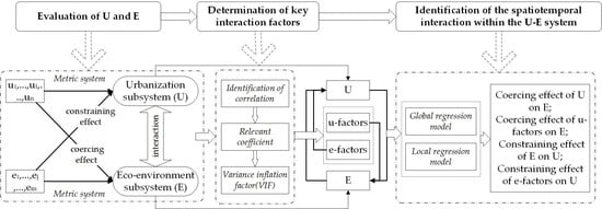
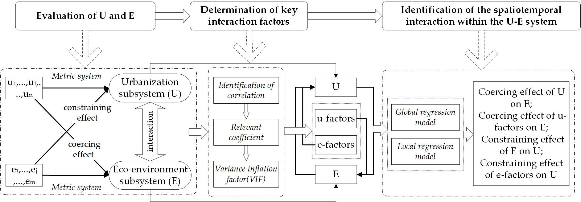
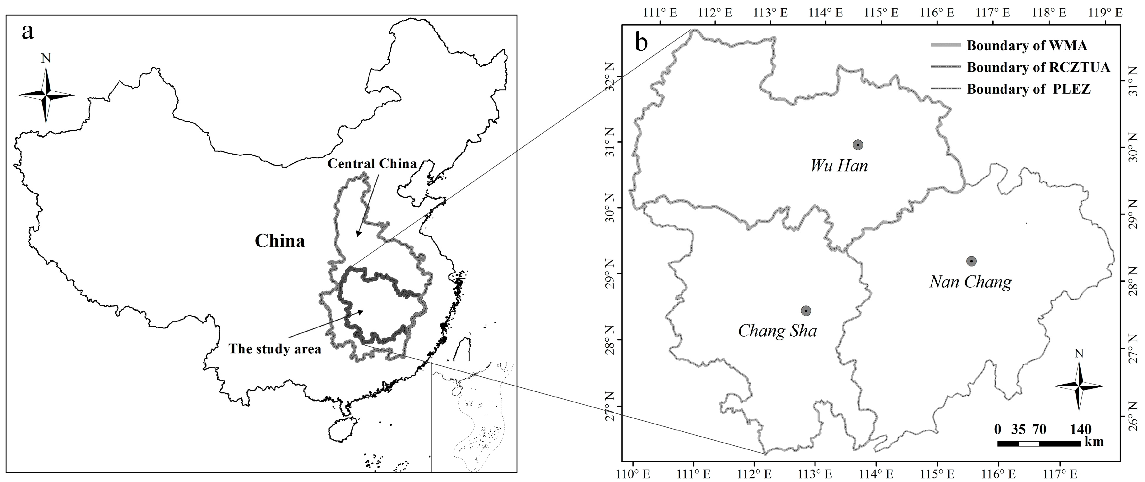
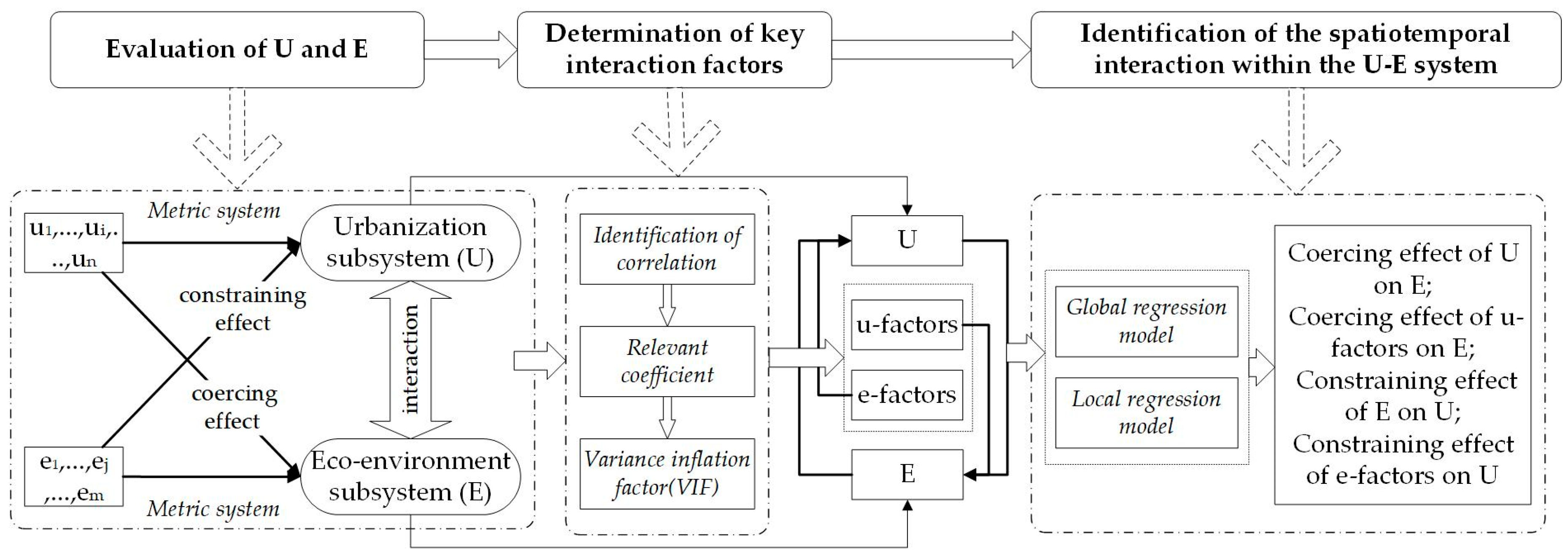
Therefore, in this study, we established such a framework to: (1) identify how U exerted coercing effects on E; (2) how E posed constraining effects on U; and (3) whether this interaction varied temporally and spatially in a UA area in China. UAMRYR, one of the five national UAs, was taken as the study region to examine the feasibility of the proposed framework and the study period covers the year of 2000 to 2015. The results of this study can provide scientific reference for policy-makers to compile effective development plans to promote regional sustainability.

2. Materials and Methods

2.1. Study Area

The UAMRYR, an important part of the economic belts of the Yangtze River, covers 31 cities across Wuhan Metropolitan Area (WMA), Ring of Chang-Zhu-Tan Urban Agglomeration (RCZTUA), and Poyang Lake Eco-economic Zone (PLEZ) in central China (see Figure 1). Wuhan, Changsha, and Nanchang are the central cities of the three sub-areas. The region is rich in resources, with the most prominent water resources and agricultural production, which provide substantial support for the development of the region. In terms of land area and population, it is the largest UA in China: it covers an area of 351,826 km², accounting for 3.30% of land in China; with a population of 128.00 million residents, it accommodates 9.31% of China’s population in 2015. The past 16 years have witnessed a rapid economic development, with GDP per capita increasing from 6671 RMB in 2000 to 52,239 RMB in 2015. As a core area in central China where new-type urbanization is promoted, it has experienced a significant upward trend in urbanization rate from 2000 (33.22%) to 2015 (55.89%). However, this rapid economic growth and urbanization have also led to increasing resource demands and a number of environmental issues [32,33,34,35].

To promote the development of central regions and the transformation of UAMRYR into a new support hub for China’s economy, regional socioeconomic plan expects UAMRYR to maintain and even accelerate ongoing development, with a goal of urbanization rate reaching 60% in 2020 (Development Plan for the UAMRYR, 2014–2020 (the State Council of China)). This means in the future, more rural population will move from rural areas to cities and share limited urban space and resources. Inevitably, this continuous migration will pose great threats on urban environment in terms of resource consumption and urban expansion, especially on the key national river basins (Poyang Lake and Dongting Lake) and the grain production base in the region. Therefore, it is urgent to examine the coupling relationship between U and E in the past years. Based on this, the government can compile scientific and detailed regional development plans to guide the protection of water resources and the steady development of agricultural bases for the sustainability of the region.

2.2. Data Pre-Processing

The Chinese government formulates a national economic plan every five years, which is called “the Five-Year Plan”. We took the end year of these plans (2000, 2005, 2010, and 2015) as the time interval of the study. The spatial data was extracted from 1:4,000,000 national geographic information database (vector-based). The socio-economic data were collected from the China City Statistical Yearbook (2001–2016), the China Statistical Yearbook for Regional Economy (2001–2016), the China Urban Construction Statistical Yearbook (2000–2015), and the Statistical Yearbook, the Statistical Bulletin on Water Resources, Statistical bulletins on the environment of provinces and cities from 2000 to 2015. We applied Formulas (1) and (2) [13,15] to standardize all the statistical data and eliminate the influence of dimension, magnitude, and positive and negative orientation.

$$\mathrm{Positive} \mathrm{indicator}: X_{ij}=(x_{ij}-\min \{x_j\})/(\max \{x_j\}-\min \{x_j\})$$

(1)

$$\mathrm{Negative} \mathrm{indicator}: X_{ij}=(\max \{x_j\}-x_{ij})/(\max \{x_j\}-\min \{x_j\})$$

(2)

where x_ij denotes the value of indicator j in year i and max{x_j} and min{x_j} represent the maximum and minimum value of indicator j for all years, respectively.

2.3. Methods

We designed a framework to examine the relationship between U and E in UAMRYR (see Figure 2). The first step is to set up an index system and calculate the overall level of the two subsystems. We then select key factors within U subsystem (u-factors) coercing E and those within E subsystem (e-factors) constraining U. Global regression (represented by the OLS approach) is adopted to examine the existence of significant interactions between U and E. If the relationship passes the significance test, local regression (e.g., GWR) is applied to further identify whether this relationship varies in space. Four groups of relationships, the coercion of U on E, the coercion of key U-factors on E, the constraint of E on U and the constraint of key E-factors on U, were investigated to address complex interactions between U and E.

2.3.1. Evaluation of U and E

Index System

The coupling between U and E is the consequence of the various interactions between the urbanized processes and eco-environmental components [19]. Measuring the urbanization process and the eco-environmental status is the basis for analyzing the impact of U on E and its response to E. Scholars have conducted a number of researches on the measurement system of U and E. Their understanding of U has also been expanded from traditional demographic urbanization and economic urbanization to the integrated urbanization that covers population, economy, space and society [10,13,14,19,36]. E is understood as a collection of resources and environment interacting with organism as well as other various elements produced in the energy flow between nature and organism [19,22]. It consists of two aspects: one is the natural environment on which humans and creatures depend, including the atmosphere, water, air, land, resources and energy; the other is the ecological elements that affect humans or organisms, including the sum of interactions among ecological structure and factors [22]. Based on this, we used four levels of indicators to represent U: demographic urbanization, spatial urbanization, economic urbanization and social urbanization. E was also represented using four levels of indicators (eco-environment level, eco-environment endowment, eco-environment pressure and eco-environment response). Further, based on the frequency of each index factor cited by the existing literature [13,21,24,29], we selected the candidate index. We then carried out principal components analysis and multicollinearity analysis on the preliminary selected indicators, to determine the main influence factors and eliminate the related indicators.

Table 1. The index system of the urbanization and eco-environment subsystems.

First Grade Index	Basic Grade Indicators (Abbreviation)	Weight (%) (2015)
Demographic urbanization	Percentage of urban population (%) (UP)	1.014
	Percentage of the secondary and tertiary industry employment (%) (STE)	1.437
Spatial urbanization	Proportion of built districts in the total land area (%) (BDP)	16.580
	Area of built districts per capita (sq.m) (PBD)	7.512
	Road surface area per capita (sq.m) (PR)	1.522
Economic urbanization	GDP per capita (Yuan) (PGDP)	3.947
	Gross industrial output value per capita (Yuan) (PIG)	4.352
	Percentage of the secondary and tertiary industry in GDP (%) (PSTG)	0.845
	Local finance income per capita (Yuan) (PFI)	6.212
	Total fixed asset investment (104 Yuan) (FAI)	10.290
Social urbanization	Total retail sales of consumer goods per capita (Yuan) (PRC)	4.407
	Disposable income of urban residents per capita (Yuan) (PDI)	0.457
	Students enrollment of regular institutions of higher education per 10,000 people (PS)	21.930
	Number of internet users per 10,000 people (PIU)	2.584
	Number of beds of hospitals per 1000 people (PB)	1.466
	Number of doctors per 1000 people (PD)	2.014
	Number of telephones users per 10,000 people (PT)	1.675
	Number of public transportation vehicles per 10,000 people (PTV)	11.755
Eco-environment level	Total volume of water per capita (m3/capital) (PW)	23.665
	Cultivated area per capita (sq.m/capital) (PC)	11.287
	Gross sown area of grain crops per capita (hm2) (PGS)	11.483
	Yield of grain crops per capita (tons/capital) (PGY)	13.328
Eco-environment endowment	Green coverage rate of built district (%) (GR)	3.491
	Green area per capita (sq.m) (PGA)	1.345
	Forest coverage (%) (FC)	16.797
Eco-environment pressure	Discharge of industrial waste water per capita * (tons/capita) (PDIW)	3.832
	Discharged volume of industrial SO2 per capita * (tons/capital) (PDIS)	3.289
	Discharged of industrial dust per capita * (tons/capital) (PDID)	5.283
Eco-environment response	Comprehensive utilization rate of industrial solid waste (%) (ISWR)	5.967
	Hazard-free treatment rate of household garbage (%) (GTR)	0.231
	Urban sewage treatment rate (%) (STR)	0.003

Note: * denotes the negative indicator, and the remainder are the positive indicators.

shows the comprehensive measurement index system, of which eighteen indicators are used for the measurement of U, thirteen indicators are for the measurement of E.

Comprehensive Evaluation

Based on the above index system, we applied an entropy method [13] to calculate the weight of each indicator for every year (Table 1), and then calculated the composite scores of U and E between 2000 and 2015 by weighted summation. The detailed formulas are as follows:

$$P_{ij}=X_{ij}/{\displaystyle \sum _{i=1}^m{X}_{ij}},(i=1,2,\dots ,m;j=1,2,\dots ,n)$$

(3)

$$w_j=\left(1+{(\ln m)}^{-1}{\displaystyle \sum _{i=1}^m\left(P_{ij}\times \ln P_{ij}\right)}\right)/{\displaystyle \sum _{j=1}^n\left(1+{(\ln m)}^{-1}{\displaystyle \sum _{i=1}^m\left(P_{ij}\times \ln P_{ij}\right)}\right)}$$

(4)

$$Y_i={\displaystyle \sum _{j=1}^n{w}_j{X}_{ij}}$$

(5)

where $P_{ij}$ is the proportion of indicator j in year i; n is the number of indicators, and m represents years; $w_j$ denotes weight of the indicator j; $Y_i$ denotes composite score in year i.

2.3.2. Determination of Key Interacting Factors within the U-E System

Interactions between U and E represent relationships between human elements within the U subsystem and natural elements within the E subsystem. It can be divided into two aspects: U impacts E by increasing resource consumption, changing land structure, producing environmental pollution, changing people’s lifestyle and concept of consumption. In turn, E has effects on U by restraining urban scale, influencing spatial layout, and restricting urban industrial structure under the constraint of ecological carrying capacity and ecological corridor.

To determine key factors in the U subsystem coercing E, we used correlation analysis and grey correlation analysis (Equations (6) and (7)) [13,15]) to calculate the correlation degree between the overall value of E and all indexes of the U subsystem listed in Table 1. Then, we removed those whose correlation coefficient and grey correlation degree were less than a threshold (0.35 here). Based on this, we applied stepwise regression analysis to quantify and eliminate the indicators whose variance inflation factor (VIF) scores were more than a threshold value (7.5 in this study). The remaining indicators were key U-factors causing coercing effects on E. The key E-factors having dominant impacts on U were determined using the same methods.

$${\xi }_{ij}\left(k\right)=\frac{\underset{j=1}{\stackrel{n}{\min }} \underset{k=1}{\stackrel{q}{\min }}\left|x_i^{\prime }\left(k\right)-y_j^{\prime }\left(k\right)\right|+\rho \underset{j=1}{\stackrel{n}{\max }} \underset{k=1}{\stackrel{q}{\max }}\left|x_i^{\prime }\left(k\right)-y_j^{\prime }\left(k\right)\right|}{\left|x_i^{\prime }\left(k\right)-y_j^{\prime }\left(k\right)\right|+\rho \underset{j=1}{\stackrel{n}{\max }} \underset{k=1}{\stackrel{q}{\max }}\left|x_i^{\prime }\left(k\right)-y_j^{\prime }\left(k\right)\right|}$$

(6)

$${\gamma }_{ij}=\frac{1}{q}{\displaystyle \sum _{k=1}^q{\xi }_{ij}\left(k\right)} (i=1,2,\dots ,m;j=1,2,\dots ,n)$$

(7)

where ξ_ij(k) represents correlation coefficient between indicator i within the U subsystem and indicator j within the E subsystem in the spatial unit k and γ_ij the average of q coefficients namely correlation degree. $x_i^{\prime }(k)$, $y_j^{\prime }(k)$ denote normalized value of indicator i within the U subsystem and that of indicator j within the E subsystem in spatial unit k, respectively. ρ is distinguishing coefficient and set to 0.5 in this study.

2.3.3. Identification of the Interaction within the U-E System

The interaction within the U-E system consists of two-way relationships: the coercion from U to E and the constraint from E to U. The relationship in each direction is divided into two aspects of influence of independent variables (its comprehensive level and inner sub-factors) on the dependent variable. Thus, we investigated four groups of interactions, namely, the coercing effect of U, key U-factors on E, the constraining effect of E, and E-factors on U.

Both OLS and GWR were adopted to examine whether each group relationship existed significantly and varied spatially. OLS, a global multivariate regression, assumes that relationships between independent and dependent variables are constant over space and thus the parameters are the same for the entire space, revealing the correlation between factors on average. Conversely, GWR, an extension of OLS, allows regression coefficients to vary in space and can describe spatial differentiation in influence of an independent variable on a dependent variable [37,38]. The following Formulas (8) and (9) are the forms of the OLS and GWR [2]:

$$y_i={\beta }_0+{\displaystyle \sum {\beta }_k}{x}_{ik}+{\epsilon }_i$$

(8)

$$y_i={\beta }_0\left(u_i,v_i\right)+{\displaystyle {\sum }_k{\beta }_k\left(u_i,v_i\right)}{x}_{ik}+{\epsilon }_i$$

(9)

where (u_i, v_i) represents the space coordinates of the sample point i; x_ik is the value of the kth independent variable in the point i; β₀ acts as intercept for the point i; β_k represents regression coefficient; β_k(u_i, v_i) stands for the value of β_k(u, v) at the sample point i; ε_i is random error term. If β_k(u, v) is spatially stationary, the equation is degenerated into a global model (8).

The fixed Gaussian kernel was used for weight estimation and cross validation (CV) was adopted to determine the optimal bandwidth. Further, whether an independent variable is global or local depends on the result of geographical variability test [39].

3. Results

We applied the proposed framework to investigate whether interactions between U and E existed and varied spatially in the study area between 2000 and 2015.

3.1. Comprehensive Level of U and E

Using the index system of the U subsystem (Table 1) and entropy method, we obtained the composite score of U for each city (Figure 3a). From the temporal change, U levels of most cities increased during the study period, with a slight growth in the first five years before rising considerably from 2005 to 2015. In terms of the spatial distribution, the regional differences of U levels were remarkable. In particular, U levels in the central cites of the three city groups in the UAMRYR, namely, Wuhan, Changsha, and Nanchang, were significantly higher than other cities in their own groups, forming a significant spatial pattern of the three pillars. In addition, WMA had the highest overall urbanization level at the regional scale. To explore the spatial characteristics of U level over the 4 years (2000, 2005, 2010 and 2015), global Moran’s I was calculated using a first-order rook neighborhood contiguity matrix (in GeoDa software). The global Moran’s I of the municipal-level U values and the corresponding p values were found to be 0.012 (0.674), −0.127 (0.381), −0.143 (0.306), −0.147 (0.289), respectively, indicating an insignificant spatial autocorrelation.

Similarly, we calculated composite values of E using the index system of E subsystem (Table 1) and entropy method. We found the spatiotemporal difference was also evident (Figure 3b). Specifically, E levels of most cities in the first decade (2000–2010) had a marked rise, while leveling off from 2010 to 2015. Spatially, the E levels of most cities in the PLEZ were significantly higher than those of the cities in the other city groups (RCZTUA and WMA) from 2000 to 2015. The results of spatial autocorrelation showed that the global Moran’s I of E levels and the p values were −0.001 (0.777), 0.422 (0.000), 0.324 (0.001), 0.274 (0.006) for the four years, illustrating a noticeably positive spatial dependence in E except in 2000.

3.2. Key Interacting Factors within the U-E System

To investigate interactions between U and E, it is necessary to determine key interacting factors within the coercing and constraining systems. We selected the average values of 4 years to avoid deviation caused by only using one-year data. Further, we transformed them into the natural logarithm to eliminate heteroscedasticity. Based on correlation analysis and grey correlation analysis combined with stepwise regression, we selected 4 key U-factors coercing E and 2 key E-factors constraining U (see

Table 2. Key interacting factors within the U-E system (VIF: Variance Inflation Factor).

Variable	Indicator	Correlation Coefficient	Grey Correlation Degree	VIF
u-factors	Percentage of urban population (UP)	−0.554 b	0.626	6.362
	Proportion of built districts in the total land area (BDP)	−0.688 b	0.521	3.186
	Total retail sales of consumer goods per capita (PRC)	−0.507 b	0.552	6.184
	Percentage of the tertiary industry in GDP(PTG)	−0.367 b	0.578	1.738
e-factors	Total volume of water per capita (PW)	−0.387 b	0.671	1.011
	Discharge of industrial waste water (PDIW)	−0.356 b	0.564	1.011

Note: ^b denotes significance at the 5% level.

). It is obvious that each selected key factor has a significant correlation with the dependent variable and there is no strong multicollinearity between variables, which shows they can be used to examine the bidirectional relationships between U and E.

3.3. Spatiotemporal Interaction within the U-E System

3.3.1. Coercing Effect of Urbanization on Eco-Environment

Effect of Urbanization Level on Eco-Environment

Taking the composite U level and E level as the independent variable and dependent variable, we employed the OLS and GWR models to examine the significance and spatial differences of the overall coercing effect from U subsystem to E subsystem.

Table 3. Summary for fitting the effect of urbanization (U) level on eco-environment (E).

Year/Model		Coefficient		Diagnosis Index
		Intercept	ln(U)	F	AIC	R2
2000	OLS	−1.020 c	−0.023	0.130	−3.943	0.004
2005	OLS	−1.173 c	−0.186 b	11.560 c	−16.388	0.285
	GWR	−1.018 a	−0.126	2.859	−38.926	0.851
2010	OLS	−1.200 c	−0.311 c	15.659 c	0.458	0.351
	GWR	−1.103 a	−0.269	3.907 a	−21.359	0.815
2015	OLS	−1.088 c	−0.337 c	19.474 c	−6.272	0.402
	GWR	−0.992 a	−0.280	3.098 a	−25.029	0.826

Note: ^a,b and ^c denote significance at the 10%, 5% and 1% levels, respectively. OLS denotes Ordinary Least Squares. GWR denotes Geographically Weighted Regression. AIC denotes Akaike information criterion.

and Figure 4 show the results.

Table 3 reports the results of regression. For 2000, the insignificant F-value and the low R² generated from the OLS analysis show that E could not be well explained only by U, whereas U exerted a significant effect on E in the next decade (2005–2015). GWR further tested the spatial distribution of this effect, and the models only for the two years (2010 and 2015) passed the significance test at the 10% level (based on the F-values), which illustrated it was until 2010 that the significant effect of U on E started to vary spatially (Figure 4). The AIC values of GWR were much lower than those of the OLS approach and their differences were more than 3. Moreover, the R² values from GWR were much higher (exceeding 80%), indicating the GWR model outperformed OLS in term of eliminating spatial dependence of variables. As observed from the results of GWR, U could explain 81.5% (2010) and 82.6% (2015) of variation in E on average and E level decreased 0.269% and 0.280% with U level increasing 1% from 2010 to 2015.

Figure 4 provides the detailed results of spatial differences derived from GWR. For most cities in the study area, the local coefficients were negative and their absolute values increased with year (see Figure 4a). The p values passed the significance test at the 10% level (Figure 4b) and the local R² values were more than 60% (Figure 4c,d). Thus, these results suggest that U caused significantly and increasingly negative influence on E. In terms of local differences, Figure 4a showed the coercing effect of U on E in the whole region was higher from southwest to northeast of the area from 2010 to 2015. More precisely, the coercion strength and the inner difference in WMA was the highest, followed by that in PLEZ and RCZTUA. The eastern and northern cities of the region are located in WMA and PLEZ, whose U levels were the highest and lowest of the study region, while E quality showed the opposite pattern (Figure 3a,b). Therefore, the generation of high-level coercing effects of U exerting on E is attributed to the urbanization process in WMA was too drastic such that the environmental degradation rate cannot keep up with its self-recovery capability. By analyzing the spatial distributions (see Figure 4b–d), we found the significance of p and strength of local R² were higher in the east than those in the west, illustrating estimated results in eastern cities outperform those in the west. Consequently, E levels might be comparatively more affected by other factors in the west of the region.

Effect of Key U-Factors on Eco-Environment

To further explore the effect of factors in the U subsystem on the E subsystem from 2005 to 2015, we carried out the OLS and GWR model with E level as the dependent variable and four key U-factors (Figure 2) as the independent variables. Before conducting GWR analysis, we used geographic variability test to determine whether independent variables should be set as global or local variables. Based on the test results, we only set the percentage of urban population (UP) indicator to a global variable for 2000, and the proportion of built districts in the total land area indicator (BDP) to global for other three years.

Table 4. Summary for fitting the effect of U-factors level on eco-environment (E).

Year	Model	Coefficient					Diagnosis Index
		Intercept	ln(UP)	ln(BDP)	ln(PRC)	ln(PTG)	F	AIC	R2
2005	OLS	0.487 c	−0.127	−0.447 c	0.347	−0.101	9.241 c	−101.837	0.587
	GWR	0.461 b	0.030 c	−0.454 a	0.275 b	−0.157 c	2.627 a	−123.603	0.889
2010	OLS	0.508 c	0.049	−0.379 b	−0.123	−0.129	6.697 c	−71.032	0.507
	GWR	0.520 c	−0.106 c	−0.335 b	0.000 c	−0.103	3.136 b	−85.722	0.780
2015	OLS	0.485 c	0.100	−0.335 b	−0.176	0.014	7.517 c	−76.697	0.536
	GWR	0.558 b	−0.154 c	−0.282 a	−0.001 b	−0.070	2.358 a	−89.253	0.803

Note: ^a,b and ^c denote significance at the 10%, 5% and 1% levels, respectively. UP denotes percentage of urban population. BDP denotes proportion of built districts in the total land area. PRC denotes total retail sales of consumer goods per capita. PTG denotes percentage of the tertiary industry in GDP. AIC denotes Akaike information criterion.

and Figure 5 report the results.

From Table 4, the F-values for all models passed the significance test at the 10% level, showing four U-factors created significant and spatially non-stationary pressure on E from 2005 to 2015. Moreover, the differences of AIC values between the two models for each year were more than 3; the R² derived from GWR were much larger than OLS. These results showed the GWR model had more remarkable capability to eliminate the spatial dependence of the residuals obtained from the linear regression model. Observed from the average coefficients derived from GWR, the influence strength of each key U factor on E could be ranked as follows: BDP > PRC > PTG > UP for 2005, BDP > UP > PTG > PRC for 2010, BDP > UP > PTG > PRC for 2015. Obviously, while the strength of proportion of built districts in the total land (BDP) indicator coercing E declined slightly (see Table 4), it had been always the maximum coercing factor compared with other three factors since 2005. In addition, from the results of significance test for U-factors, the effects of the three factors (UP, BDP, and PRC) on E were significant and spatially different on average, whereas percentage of the tertiary industry in GDP (PTG) had no remarkable influence on E. Further, Figure 5 illustrates the spatial difference of the coercion of UP, BDP and PRC.

It is noticeable that the effects of the U-factors on E varied across space according to Figure 5a1,b1,c1. Further significance of the local estimates was examined using the pseudo t test (Figure 5a2,b2,c2). The explanatory power from 2005 to 2015 was spatially non-stationary (Figure 5d1,d2,d3). Next, we analyzed in detail the spatiotemporal variation of the effect of each factor on E.

Figure 5a1 demonstrated that the negative coercion from percentage of urban population, an important indicator of demographic urbanization, to E in the region of PLEZ was the most remarkable in 2005, followed by RCZTUA and WMA where E in many cities experienced the positive influence brought by percentage of urban population. This shows that in the initial stage of development, demographic urbanization and eco-environment in WMA were in a state of harmonious development. The region of WMA experienced a rapid upward trend in the negative effect of percentage of urban population on E during 2005–2015 and this negative effect became the worst in 2015. During this period, the contradiction between the rapidly increasing population urbanization and the eco-environment in WMA continued to deteriorate. On the contrary, this decade witnessed a slight fluctuation in the effect of percentage of urban population on E in RCZTUA.

From Figure 5b1,b2, the effects of proportion of built districts in the total land area on E in the northwest and southeast regions of the cities were notably larger than those in RCZTUA in 2005. This was similar to that of the overall U level on the eco-environment, indicating that proportion of built districts in the total land area was the most crucial U-factor. For the year of 2010 and 2015, we set proportion of built districts in the total land area as a global variable because geographical variability test, indicates that spatial differences does not exist for this indicator.

In terms of the spatial distribution of the coercion from total retail sales of consumer goods per capita to E (Figure 5c1,c2), we found that total retail sales of consumer goods per capita had a negative effect on E for cities in the west part of the study region while a positive effect on E in those cities in the east part in 2005. The most serious coercion from this U factor occurred in WMA. Total retail sales of consumer goods per capita, to a certain extent, represents the quality of life, and its development has a coercive effect on the eco-environment, mainly due to that the increase in demand for infrastructure leads to more resource consumption. However, the coercion intensity of total retail sales of consumer goods per capita declined and kept at a lower level in the next years (2010 and 2015) and the largest coercing effect gradually shifted from the northwest to the east of the entire region. This shows that the infrastructure in PLEZ has been gradually improved to meet people’s demand on quality of life.

From the spatiotemporal variation of the local R² (Figure 5d1,d2,d3), we can see the local R² values were high (the maximum is over 60%) and spatially non-stationary. The explanatory power was stronger from the northwest clockwise to the southeast.

3.3.2. Constraining Effect of Eco-Environment on Urbanization

Effect of Eco-Environment Level on Urbanization

To investigate the constraining effect of E on U, we set up the OLS and GWR model with E level as the independent variable and U as the dependent variable.

Table 5. Summary for fitting the effect of eco-environment level on urbanization.

Year/Model		Coefficient		Diagnosis Index
		Intercept	ln(E)	F	AIC	R2
2000	OLS	−2.675 c	−0.197	0.130	63.112	0.004
2005	OLS	−3.319 c	−1.530 c	11.560 c	48.891	0.285
	GWR	−3.213 a	−1.490 b	1.344	48.522	0.325
2010	OLS	−2.443 c	−1.126 c	15.659 c	40.296	0.351
	GWR	−2.383	−1.126	1.073	40.233	0.385
2015	OLS	−2.077 c	−1.192 c	19.474 c	32.871	0.402
	GWR	−2.026	−1.181	0.668	33.471	0.423

Note: ^a,b and ^c denote significance at the 10%, 5% and 1% levels, respectively. The coefficients for GWR are average coefficients.

depicts the model results.

From Table 5, the constraining effect of E level on U was not obvious in 2000 but significant from 2005 to 2015 according to the F-values of OLS. Further observed from the results of the GWR model, the effect remained spatially stationary during the study period. Comparatively, the OLS model was more suitable to fit the effect of E level on U than GWR, although the latter was a little higher but actually at a relatively low performance in terms of the AIC value and R² (the maximum is only 42.3%). The results from the OLS analysis showed E can only explain 28.5%, 35.1% and 40.2% of U, and U level decreased 1.530%, 1.126% and 1.192% with E level increasing 1% from 2005 to 2015. Overall, Table 5 indicates that E might not be the main constraining factor for the change of U levels in the study region during the study period.

Effect of Key E-Factors on Urbanization

Considering that E exerted significantly negative effects on U only during 2005–2015 and there was no considerable spatial variation in these effects, we only employed the OLS approach to explore the effect of the two E-factors on U for the three years (2005, 2010 and 2015). The results were described in

Table 6. Summary for fitting the effect of E-factors levels on urbanization.

Year	Coefficient			Diagnosis Index
	Intercept	ln(PW)	ln(PDIW)	F	AIC	R2
2005	0.230 c	−0.257 b	−0.102	2.777 a	−66.517	0.166
2010	0.416 c	−0.256 b	−0.295 a	3.780 b	−52.063	0.213
2015	0.555 c	−0.413 c	−0.354 a	5.031 b	−41.815	0.264

Note: ^a,b and ^c denote significance at the 10%, 5% and 1% levels, respectively. PW denotes total volume of water per capita; PDIW denotes discharge of industrial wastewater.

.

According to Table 6, all the three OLS models passed the significance test at 10% level, and so did the two E-factors (PW and PDIW indicator) in 2010 and 2015. This illustrates that the key factors within E subsystem had remarkable influence on U. However, the R² values were relatively low such that the variation of U could not be well explained, showing the constraint influence of the two E-factors on the urban development of the study area was not that important.

4. Discussion

4.1. Necessity of the Framework

The continuous process of U exerts various coercing influences on E. In fact, E, as with the driving force of economic development, plays a crucial role in the rate of urban growth. However, the existing literature mainly focused on the unidirectional or univariate relationship from U to E, and ignored the realistic bidirectional interacting mechanism between the two subsystems. This may lead to the problem of biased estimation [31]. Therefore, the bidirectional relationships between U and E are an urgent issue to be addressed. In this article, we extended on the one-way approach and built a conceptual framework to reveal the bidirectional relationships within the complex U-E system.

4.2. Feasibility of the Framework

We applied the proposed framework to investigate spatiotemporal interaction between U and E in UAMRYR. The first step was to establish the index system of U and E, as recognized by many scholars. Next came the determination of the key factors between the two interacting subsystems. The case study showed that the key coercing factors within the U subsystem included UP, BDP, PRC and PTG, and the key constraining factors within the E subsystem involved PW and PDIW. These results are basically consistent with previous studies [11,15,40], showing the usability of the framework. The third step was the examination of the interaction. Our framework used OLS as a global regression approach to identify whether or not interacting relationships significantly existed, and further adopted GWR as local regression to examine their spatial differences. Our application in the UAMRYR showed there were significant bidirectional relationships between U and E during the last decade of the study period. In the direction of U to E, U exerted significant threats on E. Further, key U-factors involving population, land and economy within the U subsystem were found to have the main influence on E, which means the coercion from U to E was developed mainly by urban population growth, land expansion, economic development. Lin et al. [40] highlighted that larger population, higher GDP and larger urban land area often lead to poorer air quality and worse environment in China, which our results are consistent with.

From E to U, E and its internal factors, in turn, had a significantly negative and spatially stable impact on U from 2005 to 2015, which went against the common sense of “natural capital” in economic theory. In fact, scholars [26,41] also found the same interesting results as our study since the so-called resource curse hypothesis had been put forward in the resource economics. According to Sachs and Andrew [41], most current explanations for the curse are based on a crowding-out logic, namely, natural resources crowd out an activity that drives urbanization development, and thus result in harm to economic growth. Therefore, we also assume that there is such a logic from E to U. Specifically, the negative impact of E on U in the study area may be due to the government’s implementation of environmental protection policies, thus limiting certain urbanization activities such as controlling land expansion and introduction of pollution industries. To verify with this hypothesis, we consulted the government planning documents and found that there are many nature reserves in this region. The government treats the study area as a natural barrier to the ecosystem and an insurmountable gap for urban development. Therefore, we believe that the result of the reverse constraint of the case study is valid because of policy interventions. However, the constraining effect did not form a strong binding force for urbanization in the study area during the study period, as seen from the low R² for fitting the effect of E on U (see Table 5 and Table 6). Further analysis demonstrated that this may be due to the good eco-environmental conditions of the study area. Damage to the environment caused by the urbanization in 2000–2015 possibly has not yet reached the carrying capacity of resources and environment.

The practical application demonstrates the feasibility and usability of the framework. The results of the case study are interpretable and correspond to the actual development patterns in the region. The interaction mechanism within the U-E system based on this framework is consistent with the conclusions of relevant scholars [11,15,40]. Moreover, the use of global and local regression of the framework combines the advantages of both. OLS is a global regression approach that allows for revealing overall relationships between variables, and GWR as local regression only needs to further analyze the spatial variation for those significant relationships. Our framework is suitable for investigation of the interaction between U and E in other administrative levels (such as countries, provinces, UA areas, or cities), as long as the sample size is sufficient for the implementation of GWR.

4.3. Limitations and Future Research Directions

There are still several limitations and corresponding future research threads in the study. First, the regional U-E system is a complex non-linear system with multiple feedbacks and interfaces. This article only explored the interaction between the final states of the two subsystems, and revealed the one-to-one (U level and E quality) and many-to-one (multiple factors of U subsystem and E quality, multiple factors of E subsystem and U level) relationship, lacking of studying the many-to-many relationship (multiple factors in the U subsystem and multiple factors in the E subsystem). We should focus on detailed modeling and quantitative identification of various causal feedback relationships which are intricate, interrelated and interdependent within the coupled system. Second, GWR in our study was carried out based on a fixed Gaussian kernel function, which may exaggerate coefficient variability [42]. Besides, bandwidth is selected by the minimum of cross validation. Comparative studies should be further carried out to consider the effects of different kernel function and bandwidth determination criteria. Finally, our framework examines spatial differences in the interaction using GWR, which requires a large number of samples, so it is applicable to the UA area that contains a sufficient number of cities, if cities are selected as research units. If the sample size is too small, it will reduce the credibility of the regression results. Other methods may be introduced to solve the problem of fewer samples. For example, the study area can be discretized in raster grids, and socioeconomic indicators are rasterized into grid cells. Then, we can take those grid cells with various attribute values as samples, and use the proposed framework to measure spatial differences of the interaction so as to meet the requirement of sample size when using GWR.

5. Conclusions

The coordinated development between urbanized development and eco-environment protection is an important issue to be solved in China’s new-type urbanization. Identifying and quantifying the impact of U on the E system as well as the reversed relationship is key to solving this issue. Based on the traditional research, which mainly focused on the impact of U on E, we proposed a quantitative analysis framework that takes into account the bidirectional interacting mechanism for investigating the influence from U to E and the constraint from E to U. After the comprehensive evaluation of U level and E quality as well as the identification of the key interacting factors in these two subsystems, this framework detects the coercion from U level and its key factors to E as well as the constraint from the quality of E and its key factors to U based on global regression (OLS here). Further, the framework employs local regression (GWR here) to examine the regional differences of the four types of relationships.

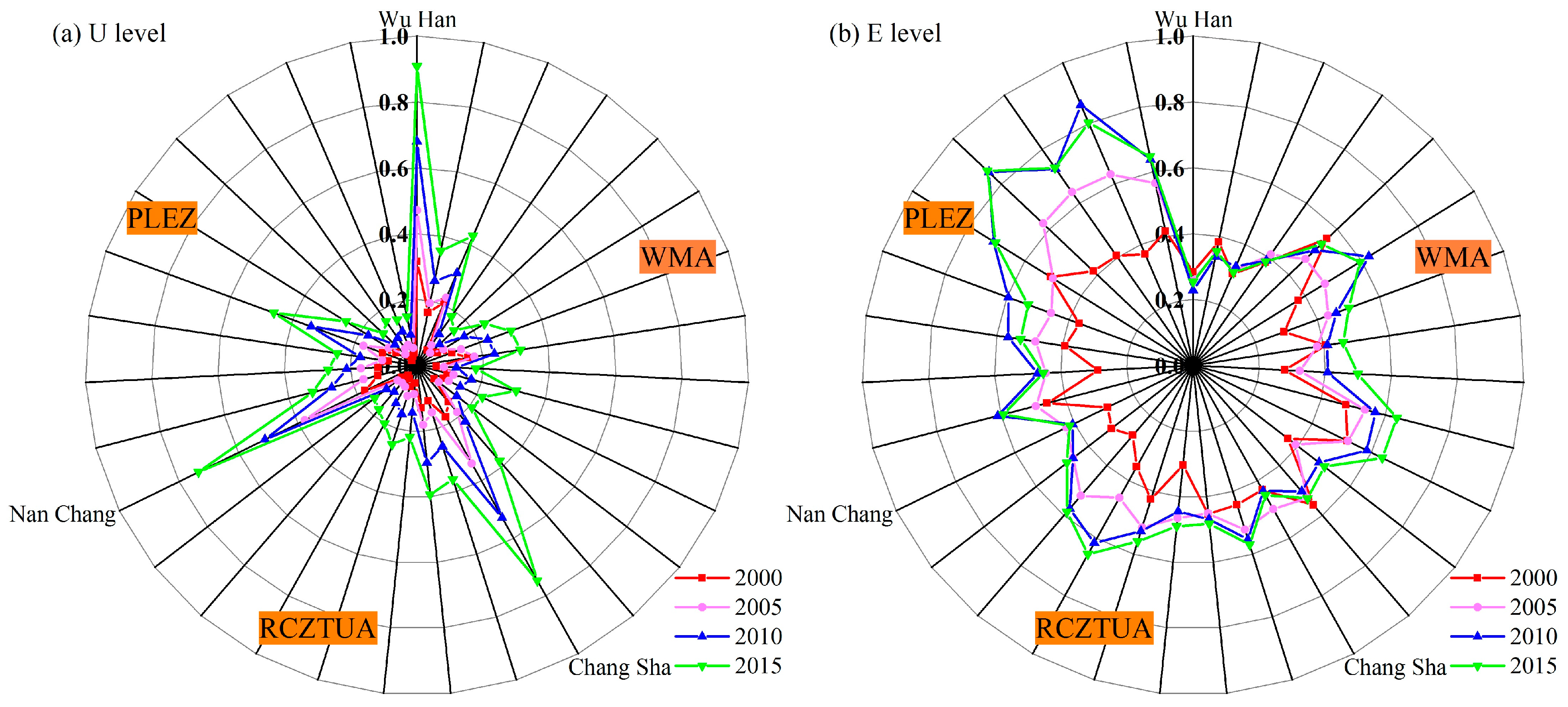
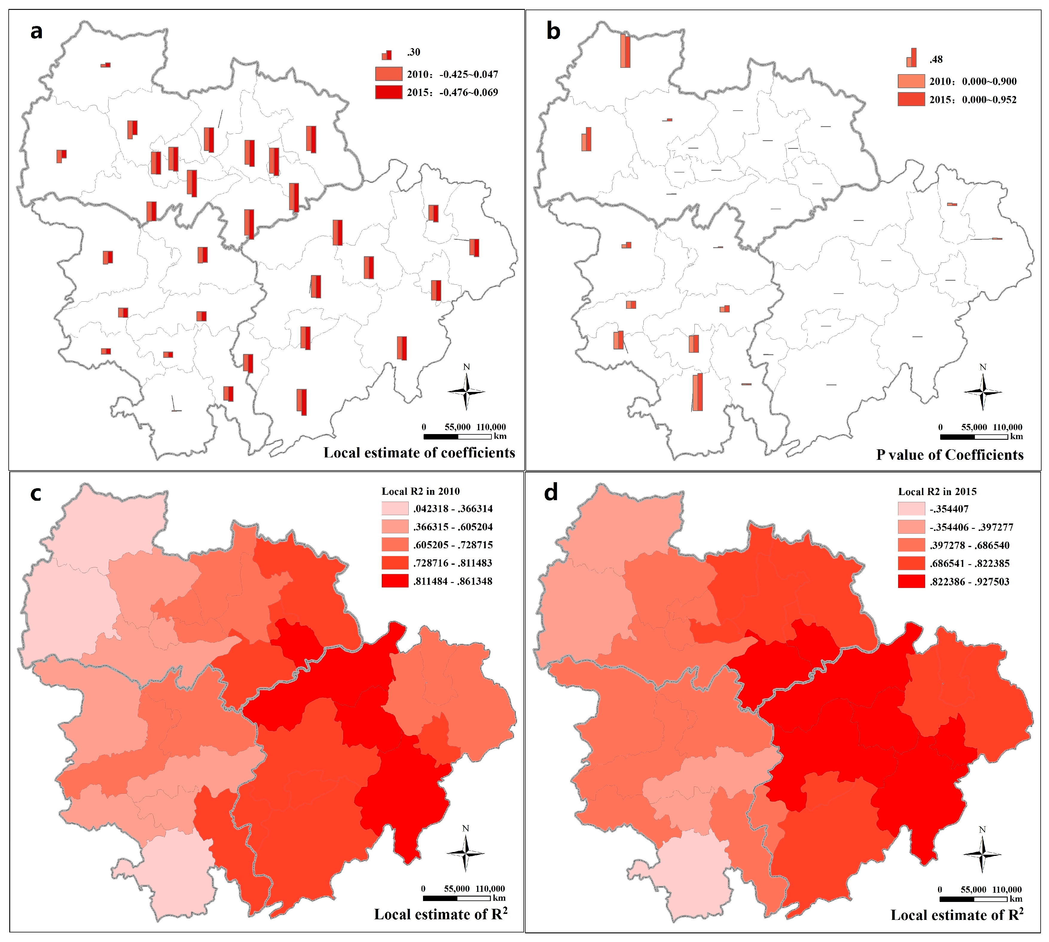
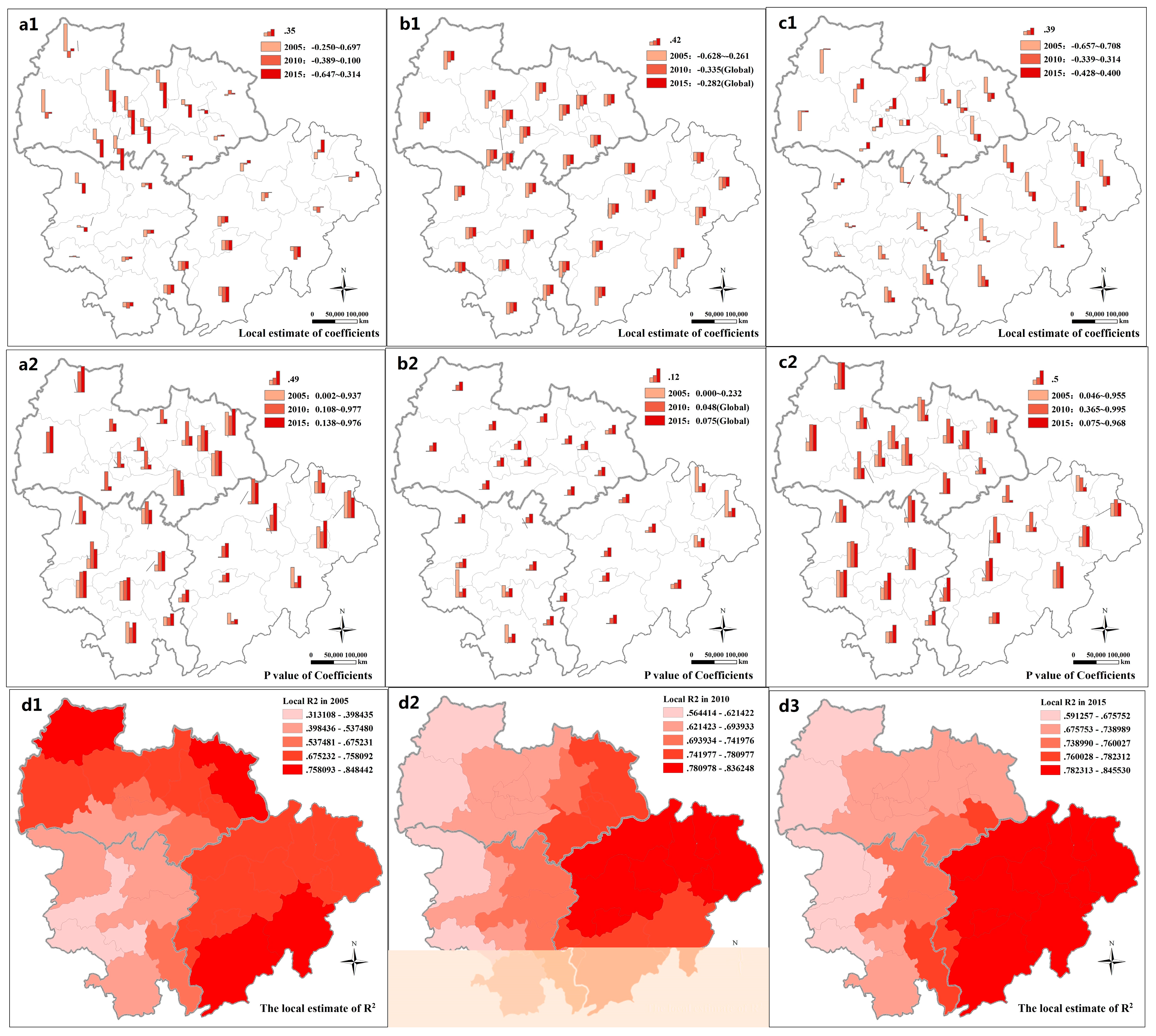
Using this proposed framework, we revealed the interaction between U and E and its spatial differences in UAMRYR during 2000–2015. From the overall relationship between the two subsystems, there was a significant coercion and restraint effect in the U-E system from 2005 to 2015. In the direction of U to E, the coercing effect increased, indicating that the impact of urbanization process on the E system got increasingly exacerbated. In terms of geographical variation in this interaction, it showed a spatial pattern of “low in southwest and high in northeast” in 2010. Comparatively speaking, this pattern became more obvious in 2015, indicating that under the different urbanization stages and eco-environmental background conditions, this influence mechanism presents different trends of development. On the other hand, in the direction of E to U, the constraining effect decreased moderately and showed a spatially stationary pattern, which demonstrated that the intensity of the constraint of E (agricultural land and water environment) on U was relatively small. This is mainly due to the good conditions of the two natural factors in the study area. In terms of influential factors, there were four key human factors (percentage of urban population, proportion of built districts in the total land area, total retail sales of consumer goods per capita and percentage of the tertiary industry in GDP) and two key natural factors (total volume of water per capita and discharge of industrial waste water) in the U-E coupling system. In the coercing direction of U-factors on E, the three factors (percentage of urban population, proportion of built districts in the total land area and total retail sales of consumer goods per capita) exerted a significant impact on E subsystem in 2005–2015. The most serious coercive factor that caused the eco-environmental deterioration was always proportion of built districts in the total land area, although the negative effect it posed became weaker during the study period. Next came percentage of urban population, which had a fluctuating effect on E. As for total retail sales of consumer goods per capita, it effected E positively in 2005, while afterwards led to increasingly negative coercion. Spatially, the impact from percentage of urban population gradually spread from PLEZ to WMA along the northwest-southeast axis of the UAMRYR region. The coercion caused by a proportion of built districts in the total land area on E showed a high level along the northwest-southeast axis but weak outside the axis in 2005. The positive effect of total retail sales of consumer goods per capita on E shifted from the east to the west of the region. In the constraining direction of E-factors on U, although the two key natural factors have a significant and spatially stable constrained effect on U from 2005–2015, they were weak in interpreting the variability of urbanization level. It can be concluded that eco-environmental change in the study area had not yet become a dominant factor constraining the development of urbanization during the study period.

The above findings of the case study will provide an important reference for the compilation of UAMRYR’s new-type urbanization plan. Population urbanization and spatial urbanization should coordinate with economic urbanization and social urbanization, so as to mitigate the negative impact of spontaneous urbanization on the ecological environment. Especially in the region of WMA and PLEZ located in the north and east of the study region, these government control efforts should be strengthened. The government should focus on immigrants’ education and employment, and realize sustainable urbanization with harmonious development of population quantity and quality. The coercion intensity of population urbanization on the ecological environment in the region of RCZTUA was the least and constantly weakened. Thus, this development mode of population urbanization should be adopted by the government of WMA. While emphasizing the expansion of urban built-up areas, more measures should be taken to focus on investing infrastructure as well as adjusting and upgrading industrial structure so as to reduce the coercion of economic development and urban expansion on the eco-environmental system. With respect to the development and construction of built-up areas, the setting of strict development threshold will be the focus of planning.

The framework provides support for investigations on the mutual interaction between U and E subsystems. Our case study demonstrated the usability and applicability of the framework. This analytical framework does not only apply to a specific region such as the study area or specific variables such as U and E in this article. Instead, this framework is useful for establishing a comprehensive understanding of the relationship between any variables as well as its spatial patterns in other regions within the context of urban sustainability.

References

1. Guan, X.L.; Wei, H.K.; Lu, S.S.; Dai, Q.; Su, H.J. Assessment on the urbanization strategy in China: Achievements, challenges and reflections. Habitat Int. 2018, 71, 97–109. [Google Scholar] [CrossRef]
2. Fang, C.L.; Liu, H.M.; Li, G.D.; Sun, D.Q.; Miao, Z. Estimating the impact of urbanization on air quality in China using spatial regression models. Sustainability 2015, 7, 15570–15592. [Google Scholar] [CrossRef]
3. Liu, Y.H.; Gao, C.C.; Lu, Y.Y. The impact of urbanization on GHG emissions in China: The role of population density. J. Clean. Prod. 2017, 157, 299–309. [Google Scholar] [CrossRef]
4. Elliott, R.J.R.; Sun, P.Y.; Zhu, T. The direct and indirect effect of urbanization on energy intensity: A province-level study for China. Energy 2017, 123, 677–692. [Google Scholar] [CrossRef]
5. Chen, M.X.; Liu, W.D.; Lu, D.D. Challenges and the way forward in China’s new-type urbanization. Land Use Policy 2016, 55, 334–339. [Google Scholar] [CrossRef]
6. Wang, X.R.; Hui, E.C.M.; Choguill, C.; Jia, S.H. The new urbanization policy in China: Which way forward? Habitat Int. 2015, 47, 279–284. [Google Scholar] [CrossRef]
7. Fang, C.L.; Zhou, C.H.; Gu, C.L.; Chen, L.D.; Li, S.C. Theoretical analysis of interactive coupled effects between urbanization and eco-environment in mega-urban agglomerations. J. Acta Geogr. Sin. 2016, 71, 531–550. (In Chinese) [Google Scholar] [CrossRef]
8. Haas, J.; Ban, Y.F. Urban growth and environmental impacts in Jing-Jin-Ji, the Yangtze, River Delta and the Pearl River Delta. Int. J. Appl. Earth Obs. Geoinf. 2014, 30, 42–55. [Google Scholar] [CrossRef]
9. Wei, Y.L.; Bao, L.J.; Wu, C.C.; He, Z.C.; Zeng, E.Y. Assessing the effects of urbanization on the environment with soil legacy and current-use insecticides: A case study in the Pearl River Delta, China. Sci. Total Environ. 2015, 514, 409–417. [Google Scholar] [CrossRef] [PubMed]
10. Zhao, Y.B.; Wang, S.J.; Zhou, C.S. Understanding the relation between urbanization and the eco-environment in China’s Yangtze River Delta using an improved EKC model and coupling analysis. Sci. Total Environ. 2016, 571, 862–875. [Google Scholar] [CrossRef] [PubMed]
11. Wang, Z.B.; Fang, C.L. Spatial-temporal characteristics and determinants of PM2.5 in the Bohai Rim Urban Agglomeration. Chemosphere 2016, 148, 148–162. [Google Scholar] [CrossRef] [PubMed]
12. Ma, S.J.; Wang, R.S. The social-economic-natural complex ecosystem. J. Acta Ecol. Sin. 1984, 4, 1–9. (In Chinese) [Google Scholar]
13. He, J.Q.; Wang, S.J.; Liu, Y.Y.; Ma, H.T.; Liu, Q.Q. Examining the relationship between urbanization and the eco-environment using a coupling analysis: Case study of Shanghai, China. Ecol. Indic. 2017, 77, 185–193. [Google Scholar] [CrossRef]
14. Li, Y.F.; Li, Y.; Zhou, Y.; Shi, Y.L.; Zhu, X.D. Investigation of a coupling model of coordination between urbanization and the environment. J. Environ. Manag. 2012, 98, 127–133. [Google Scholar] [CrossRef] [PubMed]
15. Zhao, D.Y.; Tong, L.J.; Qiu, F.D.; Guo, F.Y. Eco-environment effect of urban expansion in Songhua River Basin. J. Geogr. Res. 2017, 36, 74–84. (In Chinese) [Google Scholar]
16. Stern, D.I.; Common, M.S.; Barbier, E.B. Economic growth and environmental degradation: The environmental kuznets curve and sustainable development. World Dev. 1996, 24, 1151–1160. [Google Scholar] [CrossRef]
17. Grossman, G.M.; Krueger, A.B. Economic growth and the environment. Nat. Bur. Econ. Res. 1994, 110, 353–377. [Google Scholar]
18. Zhou, Y.X. Discussion on the regularity of relationship between urbanization and Gross National Product. Popul. Econ. 1982, 3, 28–33. (In Chinese) [Google Scholar]
19. Huang, J.C.; Fang, C.L. Analysis of coupling mechanism and rules between urbanization and eco-environment. J. Geogr. Res. 2003, 22, 211–220. (In Chinese) [Google Scholar]
20. Wang, Q.S.; Yuan, X.L.; Lai, Y.H.; Ma, C.Y.; Ren, W. Research on interactive coupling mechanism and regularity between urbanization and atmospheric environment: A case study in Shandong Province, China. Stoch. Environ. Res. Risk Assess. 2012, 26, 887–898. [Google Scholar] [CrossRef]
21. Wang, S.J.; Ma, H.T.; Zhao, Y.B. Exploring the relationship between urbanization and the eco-environment—A case study of Beijing–Tianjin–Hebei region. Ecol. Indic. 2014, 45, 171–183. [Google Scholar] [CrossRef]
22. Song, X.F.; Liu, Y.B. Scenarios simulation of urbanization and ecological environment coupling in Jiangsu province by system dynamic model. Syst. Eng. Theory Pract. 2006, 26, 124–130. (In Chinese) [Google Scholar]
23. Güneralp, B.; Seto, K.C. Environmental impacts of urban growth from an integrated dynamic perspective: A case study of Shenzhen, South China. Glob. Environ. Chang. 2008, 18, 720–735. [Google Scholar] [CrossRef]
24. Liu, Y.B.; Yao, C.S.; Wang, G.X.; Bao, S.M. An integrated sustainable development approach to modeling the eco-environmental effects from urbanization. Ecol. Indic. 2011, 11, 1599–1608. [Google Scholar] [CrossRef]
25. Xu, X.L.; Xu, X.F.; Chen, Q.; Che, Y. The impact on regional “resource curse” by coal resource tax reform in China—A dynamic CGE appraisal. Resour. Policy 2015, 45, 277–289. [Google Scholar] [CrossRef]
26. Liu, Y.B. Is the natural resource production a blessing or curse for China’s urbanization? Evidence from a space–time panel data model. Econ. Model. 2014, 38, 404–416. [Google Scholar] [CrossRef]
27. Wang, Y.; Li, L.; Kubota, J.; Han, R.; Zhu, X.D.; Lu, G.F. Does urbanization lead to more carbon emission? Evidence from a panel of BRICS countries. Appl. Energy 2016, 168, 375–380. [Google Scholar] [CrossRef]
28. Wu, Y.Z.; Zhang, X.L.; Shen, L.Y. The impact of urbanization policy on land use change: A scenario analysis. Cities 2011, 28, 147–159. [Google Scholar] [CrossRef]
29. Ren, L.J.; Cui, E.Q.; Sun, H.Y. Temporal and spatial variations in the relationship between urbanization and water quality. Environ. Sci. Pollut. Res. 2014, 21, 13646–13655. [Google Scholar] [CrossRef] [PubMed]
30. Wang, Q.S.; Yuan, X.L.; Zhang, J.; Mu, R.M.; Yang, H.C.; Ma, C.Y. Key evaluation framework for the impacts of urbanization on air environment—A case study. Ecol. Indic. 2013, 24, 266–272. [Google Scholar] [CrossRef]
31. Dinda, S. Environmental Kuznets Curve Hypothesis: A Survey. Ecol. Econ. 2004, 49, 431–455. [Google Scholar] [CrossRef] [Green Version]
32. Ding, L.; Zhao, W.T.; Huang, Y.L.; Cheng, S.G.; Liu, C. Research on the coupling coordination relationship between urbanization and the air environment: A case study of the area of Wuhan. Atmosphere 2015, 6, 1539–1558. [Google Scholar] [CrossRef]
33. Wu, H.; Ye, L.P.; Shi, W.Z.; Clarke, K.C. Assessing the effects of land use spatial structure on urban heat islands using HJ-1B remote sensing imagery in Wuhan, China. Int. J. Appl. Earth Obs. Geoinf. 2014, 32, 67–78. [Google Scholar] [CrossRef]
34. Jiang, W.G.; Chen, Z.; Lei, X.; He, B.; Jia, K.; Zhang, Y.F. Simulation of urban agglomeration ecosystem spatial distributions under different scenarios: A case study of the Changsha–Zhuzhou–Xiangtan urban agglomeration. Ecol. Eng. 2016, 88, 112–121. [Google Scholar] [CrossRef]
35. Michishita, R.; Jiang, Z.B.; Xu, B. Monitoring two decades of urbanization in the Poyang Lake area, China through spectral unmixing. Remote Sens. Environ. 2012, 117, 3–18. [Google Scholar] [CrossRef]
36. Fang, C.L.; Wang, J. A theoretical analysis of interactive coercing effects between urbanization and eco-environment. Chin. Geogr. Sci. 2013, 23, 147–162. [Google Scholar] [CrossRef]
37. Brunsdon, C.; Fotheringham, S.; Charlton, M. Geographically Weighted Regression-Modelling Spatial Non-Stationarity. J. R. Stat. Soc. 1998, 47, 431–443. [Google Scholar] [CrossRef]
38. Mcmillen, D.P. Geographically Weighted Regression: The Analysis of Spatially Varying Relationships. Am. J. Agric. Econ. 2002, 86, 554–556. [Google Scholar] [CrossRef]
39. Hu, S.G.; Yang, S.F.; Li, W.D.; Zhang, C.R.; Xu, F. Spatially non-stationary relationships between urban residential land price and impact factors in Wuhan city, China. Appl. Geogr. 2016, 68, 48–56. [Google Scholar] [CrossRef]
40. Lin, G.; Fu, J.Y.; Jiang, D.; Hu, W.S.; Dong, D.L.; Huang, Y.H.; Zhao, M.D. Spatio-Temporal Variation of PM2.5 Concentrations and Their Relationship with Geographic and Socioeconomic Factors in China. Int. J. Environ. Res. Public Health 2014, 11, 173–186. [Google Scholar] [CrossRef] [PubMed]
41. Sachs, J.R.D.; Andrew, W.M. The curse of natural resources. Eur. Econ. Rev. 2001, 45, 827–838. [Google Scholar] [CrossRef]
42. Foody, G.M. Geographical weighting as a further refinement to regression modelling: An example focused on the NDVI–rainfall relationship. Remote Sens. Environ. 2003, 88, 283–293. [Google Scholar] [CrossRef]
Figure 1. Location of study area: (a) relative location in China; and (b) urban agglomeration of the middle reaches of the Yangtze River (WMA: Wuhan Metropolitan Area; RCZTUA: Chang-Zhu-Tan Urban Agglomeration; PLEZ: Poyang Lake Eco-economic Zone).
Sustainability 10 00290 g001
Figure 2. Conceptual framework.
Sustainability 10 00290 g002
Figure 3. Comprehensive levels: (a) urbanization level; and (b) eco-environmental quality of 31 cities in different years.
Sustainability 10 00290 g003
Figure 4. Spatiotemporal variation of the parameters estimated from the geographically weighted regression model of urbanization levels: (a) local estimates; (b) p values; (c) local R2 in 2010; and (d) local R2 in 2015.
Sustainability 10 00290 g004
Figure 5. Spatiotemporal variation of the parameters estimated from the geographically weighted regression model of three significant U-factors. (a1,a2): local estimates and of p values of percentage of urban population (UP); (b1,b2): local estimates and p values of proportion of built districts in the total land area (BDP); (c1,c2): local estimates and p values of total retail sales of consumer goods per capita (PRC); and (d1d3): local R2 in 2005, 2010, and 2015.
Sustainability 10 00290 g005