Are Investments in Basic Infrastructure the Magic Wand to Boost the Local Economy of Rural Communities from Romania?

Abstract

This article investigates if public investments in rural basic infrastructure represent the best strategy for boosting the local economy of rural communities from Romania. The article focuses on one specific program implemented under the Cohesion policy in the framework of the National Plan for Rural Development, called Measure 322. Geographically, the research included a sample of rural communities from the North-Western Region of Romania. Moreover, the study also looks at other determinants of local economic development (LED), rather than infrastructure investments, with a focus on certain features characterizing Romanian rural communities such as population size, isolation from urban centers, connection with European and national roads networks, educational stock, etc. The research included three steps, namely the construction of the LED Index, a cvasi-experimental research, and a regression model. Our main findings seem to suggest that, while investments in infrastructure do help, the development gap between beneficiaries and non-beneficiaries remains relatively the same. In terms of determinants of LED level, percentage of population with a university degree and connection to a European road are the most significant in the Romanian rural context.

1. Introduction

A recent report by the World Bank describes a troublesome reality regarding the uneven social and economic development of the regions in Romania, noting that there are ‘widening disparities in economic opportunity and poverty across these regions and between urban and rural areas’ [1] (p. 1). The report talks about two different worlds, one consisting of big bustling cities (capital city Bucharest and a few secondary cities such as Cluj-Napoca, Iasi, and Timisoara), the other one of small urban towns and numerous rural communes. The urban–rural divide is extremely concerning since Romania remains one of the least urbanized countries in the European Union (hereafter EU) with approximately half of its population living in rural areas and with a relatively immobile rural population (at least statistically) [2]. The rural areas suffer, amongst other factors, from poor access to public services, an infrastructure gap, and from generalized poverty.

This article offers an in-depth investigation of the infrastructure gap of rural communities in Romania, which lack not only economic infrastructure but also social and cultural infrastructure. Road infrastructure is poor nationwide—Romania ranks 120 out of 137 countries in the quality of transport infrastructure [3] (p. 247). However, in rural communities the situation is worse—at the end of 2011, only 7% of the communal roads were modernized, the majority of the roads being either dirt roads (29%) or paved with stone (48%) [4]. The situation is very dramatic especially in the mountain regions, where communities are extremely scattered and far away from major urban centers and access to basic services depends on road accessibility and connectivity. Sewage and water infrastructure are also problematic—one in five rural people lack access to potable water, and a third live without access to a flush toilet [5]. Territorial disparities with regard to access to different types of infrastructure exist among rural communities—for example, the most affected communities by the lack of water infrastructure are the ones from the South and North-Eastern parts of Romania, where less than 1% of households have access to potable water [6] (pp. 64–67). Social infrastructure is deficient as well, social spending becoming increasingly skewed towards pensions for the elderly [5]. Nationwide, in 153 rural communities the population lacks access to health services [6] (p. 45); in 2011, in rural communities, there were 524 health care units dedicated to assisting adult patients, out of which only 27 units were dedicated specifically to the elderly. Also, in rural communities there were only 295 nurseries, which explains why less than 5% of children in rural areas are enrolled in any form of childcare [7] (p. 67). While a variety of classifications of infrastructure are available in the literature [8,9,10], in this article we will examine only basic physical infrastructure which includes local roads, water and sewage networks.

Numerous publicly funded programs (either by the Romanian Government or through Structural Funds from the EU) addressed the need to develop basic infrastructure in the rural areas of Romania as a way to boost local economic development and to improve quality of life for rural residents. These programs differ in how they select the eligible rural communities for taking part in the scheme, the type of infrastructure financed (one or multiple types of infrastructure), and whether or not they allow rural communities to partner. These programs include: SAPARD program (Measure 2.1), National Program for Rural Development 2007–2013 (Measure 322), Program for Development of Infrastructure in Rural Areas (Government Ordinance no. 7/2006), National Program for Local Development (Government Emergency Ordinance no. 28/2013). This article will specifically look into the impact of infrastructure investments made under Measure 322 and completed by 2013. Measure 322 is focused on three types of infrastructure investments—construction and modernization of basic infrastructure, development of basic community infrastructure for recreation, education, health care, etc., and preservation of cultural built heritage from rural areas. Measure 322, as opposed to the other programs, allows for different types of infrastructure to be built simultaneously (integrated approach), for small local communities to partner with each other in order to make some investments more sustainable, and gave preference during the selection process to the poorest communities. In many ways, Measure 322 tried to address some of the limitations previously identified in connection with infrastructure investments schemes, however some of the assumptions it used (such as that partnerships among local authorities increase implementation capacity and efficiency post-implementation) were never tested before including them into the financing scheme.

There is very little follow-up in terms of monitoring and evaluation of the results of these programs in Romania. Despite the fact that all of them intend to enhance the level of local economic development, the attractivity of rural communities, as well as to reduce poverty and increase quality of life for residents, there is very little relevant data in terms of the economic and social impact these programs have created [10]. Some of the ex-post evaluation documents focus rather on immediate results—such as the number of kilometers of road or sewage network created. When outcomes are evaluated, it is debatable if they are really relevant for local economic development or quality of life [11]. This situation is not unique to Romania and it can be encounter in other former communist countries experiencing significant territorial disparities [12,13]. Moreover, there seems to be little distinction between the objectives followed by these programs—economic development and poverty reduction are very often lumped together with improvements in quality of life, depending on which data is available post-implementation.

This article investigates the link between basic infrastructure investments and local economic development in rural communities from Romania, with a specific focus on North-Western Region. In light of the proposed public funding for programs supporting basic infrastructure in rural areas, it is important to know if the objective of generating economic growth is reached in this way and what factors embedded in the local context further support or hinder local economic development. Numerous studies describe proper infrastructure as one of the determinants of local economic development [14,15,16,17,18] and a precondition for improving quality of live and reducing poverty [19,20]. In the Romanian context, there is growing concern that the current poor state of rural infrastructure brings a double limitation for the country in terms of its future development—‘a drag on the international competitiveness of the more dynamic areas of Romania while limiting economic opportunities in lagging and rural areas’ [1] (p. 1). While the impact infrastructure investments have on local economic development is more clearly established, there are other determinants of local economic growth which need to be taken into consideration—existing infrastructure stock, education level of the population and social capital, type of financing and administration of the programs, whether different types of investments are integrated or not with each other, level of corruption, legal framework, coordination among various levels of government/administration and governance arrangements, etc. [21,22,23].

The main research objectives of this article are: (1) to build an index for measuring local economic development in the rural communities from Romania; (2) to assess, based on the index described under (1) if publicly funded programs aimed at building basic infrastructure (water, sewage, transport, etc.) in rural communities contribute to their economic development and poverty reduction; and (3) to determine which existing factors in the analyzed local rural communities can explain the level of economic development besides infrastructure investments and how they should be taken into consideration when deciding/prioritizing publicly funded infrastructure projects by the central governments and donors.

The remainder of the article is organized as follows: Section 2 includes a literature review focused on the role of infrastructure investments on boosting local economic development (hereafter LED) as well as on factors which act as determinants of LED. Section 3 is dedicated to methodology; the study includes a three steps research design, in line with the aforementioned research objectives. Section 4 includes a discussion of the main findings, while Section 5 concludes the article with possible suggestions for policy makers at national and European level, on how to structure the future programs aimed at fostering economic development in rural areas.

2. Literature Review

The effects of investments in infrastructure on economic growth represent a subject that has been debated for a long time in the literature. Poor infrastructure is likely to be associated with poverty pockets, and to hinder the economic development of communities, while investments are expected to stimulate economic growth through improving the competitiveness of local firms and stimulation of new economic activity creation (by improving trade opportunities, and reducing firms’ costs), thus increasing employment opportunities, and providing better jobs for residents. The authors of [24] consider public capital as an element in the macroeconomic production function. Stocks of public capital may enter in the production function directly, as an input, or may influence the productivity of multiple factors, implicitly production, indirectly. Infrastructure development has proven to be a major determinant of economic growth, in both advanced and developing countries.

In terms of empirical findings that link infrastructure investment and economic growth, Aschauer [25] is one of the most cited authors. His study, concerning the 1949 to 1985 period considers the relationship between aggregate productivity and stock and flow government-spending variables in the United Sates. The results of the study show that public investments in infrastructure positively impact the private sector growth—the core infrastructure (streets, highways, airports, mass transit, sewers, water systems, etc.) having the highest explanatory power for productivity (a 1% increase in public capital might increase total factor productivity by 0.4%). Distinguishing between military and non-military spending, Aschauer explained a general decline in productivity growth in the US in the 1970s as being caused by a decrease in productive government services.

As a reaction to Aschauer’s research, several authors have criticized the findings of his study, arguing that the evidence is not clear—due to problems regarding its methodology (many econometric uncertainties), or the unclear direction of causation between public investment and output—thus making it very hard to attribute the productivity slowdown to a shortage of infrastructure investment [15,26]. Another criticism came from studies using more sophisticated econometric techniques [27,28,29,30] which challenged the significance of Aschauer’s results in terms of providing a clear indication for policy that, in general, public investment in infrastructure positively affects growth.

The author of [31] was one of the pioneers of introducing public expenditures into economic growth models, concluding that endogenous growth could be induced by public expenditure represented by infrastructure. Using an approach based on the growth model developed by Barro, the authors of [17] address the issue of an optimal threshold or growth maximizing the level of infrastructure stock. Using country data spanning from 1950 to 1992 (GDP per worker for growth, and roads, electricity generating capacity and number of telephones for infrastructure), the authors find that due to the fact that infrastructure capital comes at the cost of reduced investment in other types of capital, if infrastructure levels are set too high, positive infrastructure shocks will tend to reduce the levels of output. In another study [32], the authors go further, investigating the consequences of infrastructure provision (using the same data panel), showing that while infrastructure tends to cause long-term economic growth, there is a substantial difference across countries (under- and over-supply).

In the same vein, the authors of [18] provide empirical proof that growth is positively affected by the stock of infrastructure assets using a panel data of 121 countries, spanning the period 1960–2000. Moreover, the research shows that income inequality declines with higher infrastructure quantity and quality. The authors use principal component analysis to build infrastructure indices (the indices are given by the first principal component of the underlying variables), which are further aggregated into an index of infrastructure stocks, and infrastructure quality, using data from transportation, power and telecommunication sectors.

At the level of the EU, a study conducted by the author of [33] indicates that infrastructure endowment is a poor predictor of economic growth. Instead, regional growth is connected with innovation capacity and migrant attraction capacity. The study uses a panel of 120 regions in EU15 countries.

Closer to our geographical area of interest, the authors of [34] conducted a study on infrastructure investments in groups of EU countries. The study (based as well on Barro’s government spending model), uses 1980–2010 data (extracted from World Bank’s World Development Indicators), analyzing the relationship between GDP growth and different types of infrastructure expenditures. The country panel was divided in two categories (EU 15 and EU 12), according to their accession to EU, an overview of the effects on EU 27 being presented in a model as well. In the study, GDP per capita growth rate is used as the dependent variable, while the independent variables are: telephone lines, air transport, rail lines, roads, and energy production. Despite that, due to the lack of data (lack of significant total road network data was mentioned as a limit of the study), the results at EU 12 groups could not identify the connection between infrastructure investments and growth, the results of the study show that telecommunications investments have positive effects on growth in all groups, energy investments have positive effects in EU 15, and EU 27 groups, while investments on railway and road have positive effects only in the EU 27 group. What we can extract from the study, and would be significant for our research and Romania’s economic development perspective, is the conclusion of the authors, namely that in EU 12 member countries (most recent members of EU at the time of the study, including Romania), the impact of additional infrastructure investment on growth is prominent due to the catch-up effect—investing on more physical capital in these countries will substantially contribute to their production.

Focusing on a single specific type of infrastructure, the authors of [35] estimate the effect of broadband infrastructure on the economic growth of 25 OECD countries during the 1996–2007 period, finding that a 10% increase in broadband penetration increased annual per capita growth by 0.9–1.5%. Using several types of models, among which a difference-in differences specification, the authors identify that GDP per capita is about 2.7–3.9% higher on average after than before broadband introduction (controlling for country and year fixed effects). The authors of [36], using difference-in differences and propensity score matching evaluation techniques, found that loans made in 2002 and 2003 under the Pilot Broadband Loan Program of the U.S. Department of Agriculture (USDA), have had a substantial positive impact on employment, annual payroll, and the number of business establishments in recipient communities. The difference-in differences fixed effects estimation was performed on the panel of zip code-level data from 1998 to 2007. The difference-in differences analysis compared the dependent variable between two groups of zip codes—a treatment group of zip codes that received a broadband loan and a control group of zip codes that did not receive a loan—before and after the treatment group received the loan.

Although at international level there is a significant body of research on assessing the impact of infrastructure on economic growth, studies focusing on the Romanian case are missing. Except for a few studies on the case of the Baltic States [37] or Poland [38], there is a scarcity of this type of study, also regarding the countries from the Central and Eastern Europe (hereafter CEE) region. However, there is an important body of literature covering developing Middle East and Asian countries, focusing not only on the national level but also on regional and local level effects of different types of infrastructure provision on economic development or poverty reduction.

Using panel data throughout the 1985 to 1998 period, a sample of 24 Chinese provinces [39] shows that geographical location and infrastructure endowment significantly accounts for observed differences in growth performance across provinces. Transport facilities are a key differentiating factor, identified by the results, in explaining the growth gap between provinces.

The authors of [40] analyze the distributive impacts of infrastructure (telephone, water and electricity) on individual income in China, providing estimates of growth and the distributive impacts of specific physical infrastructures. The results show that all infrastructures helped raise rural income, income gains differing for different population groups. In an attempt to examine the effects of several types of government expenditures on growth and rural poverty in China, using province-level data, the authors of [41] found that investment in rural roads significantly reduce poverty incidence through agricultural productivity and nonfarm employment. Estimating elasticity coefficients for agricultural and non-agricultural GDP per worker, and for wages of nonagricultural workers in relation to road infrastructure density, the authors found that rural roads projects have the largest impact (among all government infrastructure projects) on poverty reduction.

Reference [42] explores eventual productivity gains in rural Kyrgyzstan using difference-in-differences estimate of the water infrastructure’s impact. Choosing a sample of 173 villages, the author is researching whether improvements in water technologies enable changes in household time allocation and, thereby, productivity gains in households.

Reference [43] evaluate the impacts of electrification in rural Vietnam. Their analysis is based on a panel survey from 2002 and 2005 for 1100 households, including in the econometric framework a difference-in-difference analysis, a difference-in-difference with fixed-effects regression and propensity score matching. The findings show significant positive impacts of electrification on households’ income, expenditures, and also on educational outcome. Previous research in the case of Vietnam [44] investigates for positive effects of road infrastructure, and finds that poor households originating in rural communes with paved roads have a 67% higher probability of escaping poverty compared to the households located in communes without paved roads.

Summing up, the studies described above vary significantly in terms of the econometric models used but also with regard to how they define economic development or growth. The latter has been measured either as a function of one specific indicator or of a complex aggregated index. Studies also differ with regard to the size of the area investigated coupled with the level of government covering that area, as well as with regard to the geographical location of the investigated communities.

Our study concerns itself not only with assessing the impact of infrastructure investments on economic growth, but also with identifying other determinants of local economic growth connected to the characteristics of the rural communities from Romania. We therefore looked at studies which also assessed the entire spectrum of local economic determinants.

Rural economic competitiveness is a complex issue, infrastructure being only one of the multiple factors of influence. The author of [23] identifies 11 factors considered to be important to local economic development: locational, physical, infrastructural, human resources, capital and finance, knowledge and technology, industrial factors, quality of life, business culture, community identity and institutional capacity. Although usually there are significant discrepancies between the economic development of urban and rural areas, the authors of [45] consider that rural areas rise or fall economically based on the same principles as other regions, so we expect that the factors which explain the economic growth to be identical. The same study identifies the fact US Rural regions are in many cases tightly linked to nearby metropolitan regions, confirming location as an important developmental factor. The authors of [46] identified several factors related to U.S. rural communities’ growth in the 1980s: attractiveness to retirees, right-to-work laws, excellent high school completion rates, good public education expenditures, and access to transportation networks. The findings related to the role of educational factors are in line with [47] study on data for 42 countries, which identify a positive role of human capital (average year of schooling of the labor force) in explaining economic growth.

Examining the determinants of economic performance of 149 English rural districts, Reference [48] identified that a range of factors of economic and human capital: productivity (skills, investment, and enterprise), spatial factors (peripherality and accessibility), and other key factors (economic structure, government infrastructure, road infrastructure, and occupational health), are significant determinants of economic performance in rural areas.

In a series of studies [49,50,51] the authors emphasize the role of SMEs in rural economic development, and the importance of innovation in rural enterprises. Their research findings show that innovative firms, through external income generation and employment generation, make an important contribution to rural economies.

3. Methodological Framework

3.1. Research Goal, Objectives and Hypotheses

This research aims to assess the connection between local economic development in rural communities from the North-Western Region of Romania and publicly funded investments in basic local infrastructure (water, sewerage, and local roads). More specifically, the analysis strives to determine if local economic development of rural communities can be enhanced through investments in infrastructure, or if other factors, linked to the local context in these communities (such as location in relation to big urban centers and access to existing networks of roads, population size, educational stock of the population in the community, etc.) need to be taken into consideration as well. The specific objectives of the study are:

O1: To build an index for measuring local economic development; the index will serve as the dependent variable in our statistical analyses.

O2: To determine the impact of investments in various types of local basic infrastructure on local economic development.

O3: To investigate other determinants of local economic development besides investments in basic infrastructure, which are closely linked with characteristics of the rural communities from Romania.

The research hypotheses are:

Hypothesis 1 (H1).

Rural communes which implemented infrastructure projects financed from Measure 322 have developed faster than the ones which did not access funds through this program.

Hypothesis 2 (H2).

Rural communities implementing integrated infrastructure projects financed from Measure 322 developed at a faster pace than those which have not accessed funding through the program, or have implemented investment projects with only one or two components.

Hypothesis 3 (H3).

During the execution/construction phase of local basic infrastructure projects the local economy of communes grows at a higher pace, compared to that of communes which have not benefited from funding.

Hypothesis 4 (H4).

The level of local economic development in rural communities from Romania is predicted by: the size of the commune’s population, direct access to national and European road networks, and percentage of university graduates in total population (educational stock).

3.2. Public Investments in Infrastructure—Measure 322, National Plan for Rural Development

Under the Cohesion Policy, Romania benefits from allocations aimed at the development of its rural areas. During the We used the same technique financial cycle 2007–2013, the National Plan for Rural Development included, among other strategies and programs, Measure 322. Measure 322 targeted investments in basic infrastructure—water systems, sewage, and local roads, in social infrastructure (i.e., kindergartens) and in cultural infrastructure (i.e., restoration of existing monuments or buildings with cultural value). The projects were awarded on the basis of competition during March 2008–May 2014. Besides meeting certain eligibility criteria, the individual projects were assessed based on a list of relevant criteria, the higher the score obtained by a project the higher the chances of being selected. The applications could be done individually by each rural community or in association. The value of the projects could be no more than 6 million euros—bonuses were given to communities for applying for integrated investments (multiple types of infrastructure) and for applying in association. It is clear that these two objectives were considered as extremely important by the Romanian government—integration of multiple types of infrastructure not just one type and association of multiple rural communities for implementing these projects as a way to counteract excessive administrative fragmentation and limited capacity in small communities. The projects included in our research were signed in 2008–2009 and the execution of the works took place from 2011 to 2013. We selected only projects completed in 2013 so as to have at least a period of three years for measuring potential impacts in the local economy. We only focused on basic infrastructure projects, excluding social infrastructure and cultural infrastructure from the study.

3.3. Location of Research

In this study we investigate the rural communities from the North-Western region of Romania. The territory of Romania is divided into 8 development regions. They were created in 1998, in the context of Romania’s accession to the EU, with the purpose of managing projects and EU funds during the pre-accession period. Despite numerous proposals for reform the structure of the regional models is still unchanged as of 2018. The regions are not self-governed bodies of local public administration, which enjoy local autonomy. They are, rather, created based on the voluntary cooperation of counties, having as main role the management of EU structural funds and the development and implementation of economic development strategies and policies at regional level. North-Western region was selected as the location of the research for multiple reasons: all 8 regions are relatively similar in size and composition of rural and urban communities, therefore results obtained in one region could be extrapolated to the other regions; access to previous studies and secondary data for this region investigating similar topics, etc.

3.4. Steps in the Analysis

3.4.1. Building the Local Economic Development (Hereafter LED) Index

For the purpose of this study, authors measured LED (dependent variable) through an index that was built and tested previously in the framework of a somewhat similar research [52], assessing the impact on local economic development of a different program financing investments in infrastructure.

Numerous definitions of LED exist in the literature. While the understanding of this concept has evolved over time, the importance attributed to the endogenous nature of the approach is notorious in all of them [53] (p. 24). Most authors highlight that LED is both a product and a process [54] (p. 4). Jobs, wealth, investment, standard of living and working conditions represent the product of economic development, while the process consists of industry support, and the development of infrastructure, labor force and markets. According to [21] (p. 3), the purpose of LED is “to build up the economic capacity of a local area to improve its economic future and to improve the quality of life for all. It is a process by which public, business and non-governmental sector partners work collectively to create better conditions for economic growth and employment generation”. Due to the holistic complex, and multidimensional nature of LED (economic, social and environmental), a single indicator that can provide an adequate measure of LED cannot be identified [23]. The authors of [55] stress that using a single indicator (for example GDP or GDP/capita) is inappropriate, because it does not take into consideration the various dimensions of LED.

Other important challenges regard the difficulty in choosing the most appropriate proxies for each LED dimension (education, environment, health, etc.), but also to establish the importance/weight of each indicator in measuring general development level. Therefore, an aggregation of individual indicators into an index becomes absolutely necessary.

In our research LED is addressed and measured as a result. The LED Index, constructed for the period 2007–2016, aggregates mostly economic indicators—indicators regard local economy and its efficiency. This is mostly due to lack of data at the local level. This is why indicators for other dimensions of LED, such as environment for example, could not be introduced in the Index. Future efforts should be aimed at measuring other dimensions of LED through quantitative and qualitative research.

In selecting and computing the indicators, we applied the following selection principles: The indicator should be already validated in the literature; The data for the indicator calculation should not be subject to errors or missing data; The indicators should be comparable, thus we weighted most of them with the size of the population.

Our proposed LED Index aggregates 10 indicators measured at the level of rural community (self-governed, autonomous bodies of local public administration). These indicators were computed based on data obtained from the National Trade Register Office, the Agency for Fiscal Policy and Local Budgeting of the Ministry for Regional Development and Public Affairs, the Romanian National Institute for Statistic and 2011 Population Census Data.

Table 1. Variables (indicators) used in the construction of the local economic development (LED) Index.

No.	Indicators (Variables)	Explanation
1	Turnover (per capita)	Turnover at the level of the commune divided by the size of the population
2	Turnover (per employee)	Turnover at the level of the commune divided by the average number of employees
3	Average number of employees (per 1000 inhabitants)	Total number of employees at the level of the commune divided by the size of the population and multiplied by 1000
4	The percentage of employees in the total working-age population	The average number of employees divided by the number of the working-age population (15–64 years)
5	Budgetary revenue from personal/company income taxes (per capita)	The total value of the budgetary revenue from personal/company income tax breakdowns at the level of the commune, divided by the size of the population
6	Budgetary revenue from local taxes (per capita)	Total budgetary revenue from local taxes at the level of the commune divided by the population size
7	Active business density	The number of enterprises divided by the size of the population and multiplied by 1000
8	Entrepreneurial capacity	The number of newly created enterprises for every 1000 people; calculated based on total number of newly created enterprises divided by size of the population and multiplied by 1000
9	Social assistance expenses (per capita)	The total social assistance expenditures at the level of the commune divided by the size of the population.
10	Number of dwellings completed during the year (per 1000 inhabitants)	The total number of dwellings completed during the year divided by the size of the population and multiplied by 1000

Source: Compiled by the authors.

below details how each indicator was built and what it measures.

Each indicator has been computed on an annual basis for each commune. In order to be comparable, the data for each commune have been adjusted with the size of the population or the number of employees where necessary, while the indicators based on monetary units (turnover per capita, turnover per employee, budgetary revenue from income tax breakdowns per capita, budgetary revenue from local taxes per capita, social assistance expenses per capita) have been updated with the inflation rate. The indicators have been aggregated using Principal Components Analysis (PCA), one of the most common methods used by data analysts to provide a condensed description and describe patterns of variation in multivariate data sets.

3.4.2. Cvasi-Experimental Research

We used a cvasi-experimental research design to determine if investments in infrastructure, considered as the treatment, determine an increase in the level of LED. The communes which have implemented projects through Measure 322 represent the treatment group, while the ones which have not are the control group. In the case of the treatment group, out of the total number of 398 (there are 403 communes in total, but 5 were excluded from the analysis because they are outliers) communes from the North-Western Region, 145 have contracted projects financed through Measure 322. However, only 64 communes have completed them, as of the end of 2013. From the treatment group we eliminated the communes which partially benefited from financing but did not complete the implementation of the projects (81 cases). In the end, the treatment group includes 64 communes. Out of these 64 communes, most of them implemented integrated projects, combining at least two types of investment: water infrastructure and sewerage infrastructure (8 cases) or water infrastructure and local roads (3 cases) or sewerage infrastructure and local roads (9 cases) or all of those three types of basic infrastructure—water, sewerage and local roads (26 cases). In 18 cases there was only one type of basic local infrastructure built, namely local roads. Also, out of the 64 communes, 11 of them implemented the projects based on association between communes. This was a feature of Measure 322, which allowed associations of communes to apply and receive higher financing.

The control group (same size as the treatment group) was built through stratified random sampling, in connection with the rank of the communes from the non-treatment group (253 cases). The rank of the commune refers to the position of a certain commune in the hierarchy of rural localities from Romania. The rank indicates the position of a commune by reference to an urban center. Communes can be located in the immediate vicinity of a big city or they can be isolated. As multiple studies have concluded, proximity to a large urban area can exert a positive influence on the surrounding rural communities, while spatial (geographical) isolation from large urban centers can often condemn deep-rural communities to underdevelopment and stagnation. The rank of the communes from the North-Western Region of Romania was determined based on a policy report prepared by the Romanian government [56]. Based on this document, we grouped the communes from the region in six categories of functional areas (along a continuum), where rank 1 includes the most isolated communes (294 communes) and rank 6 includes the communes located near a large city with a minimum of 100,000 inhabitants (50 communes).

Out of the 64 communes which completed the implementation of the projects financed from Measure 322, 51 (79.7%) of them are rank 1 communes (isolated communes), while the rest of the sample include ranks 2, 3, 4, 5 and 6 (2 communes in rank 2, 1 commune in rank 3, 5 communes in rank 4, 1 commune in rank 5, and 5 communes in rank 6). The control group has the same size and it was created through aleatory stratified sampling in order to mirror the structure of the treatment group.

In order to assess the difference between the treatment group and the control group, we used the difference-in-differences technique, an intuitive technique mostly used to assess the impact of policies and programs. Before conducting the difference-in-differences technique, we verified the normality of value distribution of the LED Index values for the period 2007–2016. The values of LED Index for 2007, 2013, 2016 and of the differences between them are not normally distributed (except for the differences between 2016 and 2007), which meant we used an equivalent nonparametric Independent Sample t-test, namely Mann–Whitney U-test, in order to compare the two independent groups, treatment and control.

3.4.3. Regression Models

As a final step in our research, using linear regression models, we assessed also if other independent variables such as direct connection to a national or European road network, population size of the commune, and percentage of university graduates in the total population act as determinants of LED.

LED determinants, both endogenous and exogenous, have all been investigated and classified previously in a variety of studies [21,22]. Infrastructure is one key factor, especially important in the Romanian context, but other determinants might be equally important. Our hypothesis is that these determinants are highly contextual and therefore they need to be identified in the context of each country/region.

Our choice of these specific determinants is based on the challenges of rural communities from Romania face in the broader context of administrative reform [57,58]. Various authors have argued that rural communities have limited administrative capacity due to fragmentation of local government (which leads to inefficiency and poor quality in the provision of local services) [54], reduced accessibility and connectivity to urban centers (more than 50% of rural communities have no urban center at a distance smaller than 25 km) [57,59], and inadequate educational stock in the community, especially by comparison with urban communities (has implications for both individuals working in public administrations as well as for potential entrepreneurs in the community) [60,61]. All of these independent variables are, for the most part, outside of the control of local administrations and therefore they need to be considered when designing public policies and programs meant to support the development and poverty reduction in these rural communities. For administrative fragmentation we included in our model as independent variable the size of the local population. For connectivity and accessibility, we used connection to a national or European road. This distinction was made because an eligibility requirement of the program was to have connection to a county road. We hypothesized therefore that the category of road, to which connection was sought, would be relevant. For the quality of the educational stock we used in the model the percentage of university graduates in the total population, an indicator which portrays, very accurately, the urban/rural divide which was described in the introductory section to this article.

These determinants have been all previously studied in the literature, with mixed results. There seems to be consensus in the literature that direct connection to a national or European road network can stimulate economic activity and economic growth [62,63,64,65,66]. The connection between the population size and LED is less clear cut, with numerous studies pointing in the direction of both positive and negative influences of this variable on LED [67,68,69,70]. Considering the size of population, the communes in the sample were grouped into six categories, as follows: Category 1—up to 1500 inhabitants; Category 2—from 1501 to 3000 inhabitants; Category 3—from 3001 to 4500 inhabitants; Category 4—from 4501 to 6000 inhabitants; Category 5—from 6001 to 7500 inhabitants, and Category 6—more than 7500 inhabitants. The percentage of university graduates (proxy for educational stock in the community) was included as an independent variable based on the findings of various studies [71,72,73,74]. This indicator was calculated based on the 2011 Population Census Data, for each commune, as a share of the total population.

4. Results and Discussion

O1 of our study was to construct an Index for measuring LED in rural communes from the North-Western Region of Romania, which however, could be then used for all rural communes in Romania. To construct the LED Index, we used factorial analysis based on principal component analysis (PCA). For each year, we used the factorial extraction based on non-fixed number of factors. To weight each indicator, we used the values of first component extracted from the matrix of PCA.

The values of first component extracted, the Kaiser–Meyer–Olkin (KMO) values, the total variance explained by the first component extracted and the total number of extracted components are included in

Table 2. The main results of PCA.

Indicators/Year	2007	2008	2009	2010	2011	2012	2013	2014	2015	2016
Factor loadings for the first component extracted
Turnover per capita	0.901	0.900	0.835	0.878	0.839	0.887	0.907	0.900	0.901	0.894
Turnover per employee	0.403	0.319	0.459	0.450	0.424	0.474	0.427	0.374	0.347	0.330
Average number of employees per 1000 inhabitants	0.894	0.921	0.930	0.925	0.927	0.939	0.957	0.941	0.938	0.947
Percentage of employees in the total working-age population	0.887	0.913	0.925	0.921	0.922	0.935	0.954	0.938	0.937	0.947
Income from income tax breakdowns per capita	0.695	0.607	0.697	0.746	0.762	0.845	0.832	0.820	0.850	0.843
Income from local taxes per capita	0.424	0.529	0.681	0.706	0.555	0.560	0.524	0.610	0.495	0.472
Active business density	0.853	0.874	0.817	0.751	0.754	0.737	0.712	0.752	0.759	0.752
Entrepreneurial capacity	0.624	0.707	0.439	0.121	0.191	0.209	0.101	0.588	0.556	0.564
Social assistance expenses per capita	−0.316	−0.306	−0.188	−0.330	−0.147	−0.093	−0.067	−0.023	0.001	−0.003
Number of dwellings completed during the year per 1000 inhabitants	0.458	0.499	0.508	0.397	0.491	0.470	0.457	0.436	0.576	0.537
Indicators
KMO	0.771	0.789	0.803	0.793	0.774	0.783	0.783	0.783	0.794	0.783
Bartlett’s Test 1 for Sphericity	3855.9	3197.1	3639.2	3816.	3662.0	3906.9	3967.7	4344.9	4444.6	4422.7
Total variance explained by the first component extracted (%)	46.504	48.480	47.295	45.575	43.503	46.117	45.294	48.628	48.723	48.070
Number of components	2	2	2	2	2	2	3	3	3	3

¹ The significance was 0.000 for each year. Source: Compiled by the authors.

.

The sampling adequacy (the KMO values) are well over 0.5 for each year, indicating the high level of adequacy of the correlation matrix and the fact that the indicators used are appropriates for aggregation using PCA, and the significance of Bartlett’s test of Sphericity (which stands at 0.000) recommend continuing the analysis. The first factor extracted in each year explains more than 43% of the total variance and the low number of extracted factors (two for six years and three for four years) further confirm that the indicators are appropriate for aggregation.

The values for the first component extracted show that the most relevant indicators used for aggregation are the average number of employees (per 1000 inhabitants), percentage of employees in the total working-age population, turnover (per capita), budgetary revenues from personal/company income tax breakdowns (per capita) and active business density; their weight is closer to 1 than to 0 and they are almost constant for all the analyzed period. Entrepreneurial capacity and social assistance expenses (per capita) are the indicators with the lowest weight (loadings) and the most inconsistent values during the analyzed period; as we expected, social assistance expenses (per capita) are negatively weighted in the first component extracted.

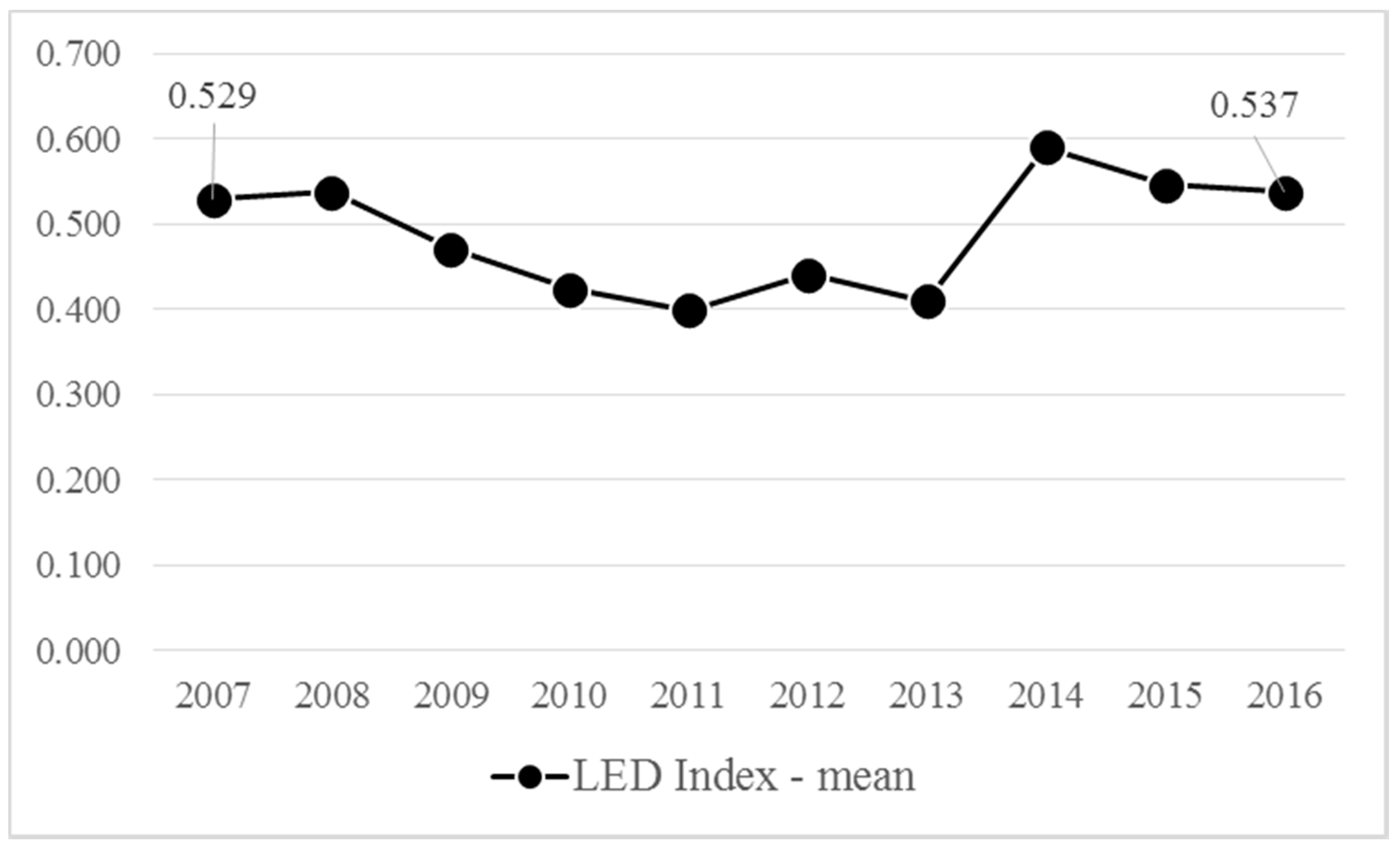
The values of the Index obtained based on factorial analysis vary significantly from one commune to another for the same calendar year, and they are not normally distributed for any of the years for which they have been computed. Annual mean values graphically presented in Figure 1 confirm the fluctuating evolution of the LED Index in the 398 communes of the North-Western Region of Romania.

In Figure 1, we can observe the drop in LED Index starting with 2008, once the economic crisis started. The trend continues until 2011, with a significant increase in 2014. The evolution of LED is in line with our expectations, given the somewhat later start of the crisis in Romania. The sharp increase in 2014, besides positive trends in the economy nationwide, can be attributed in rural communities also to a more accelerated absorption of EU funds under the Cohesion policy.

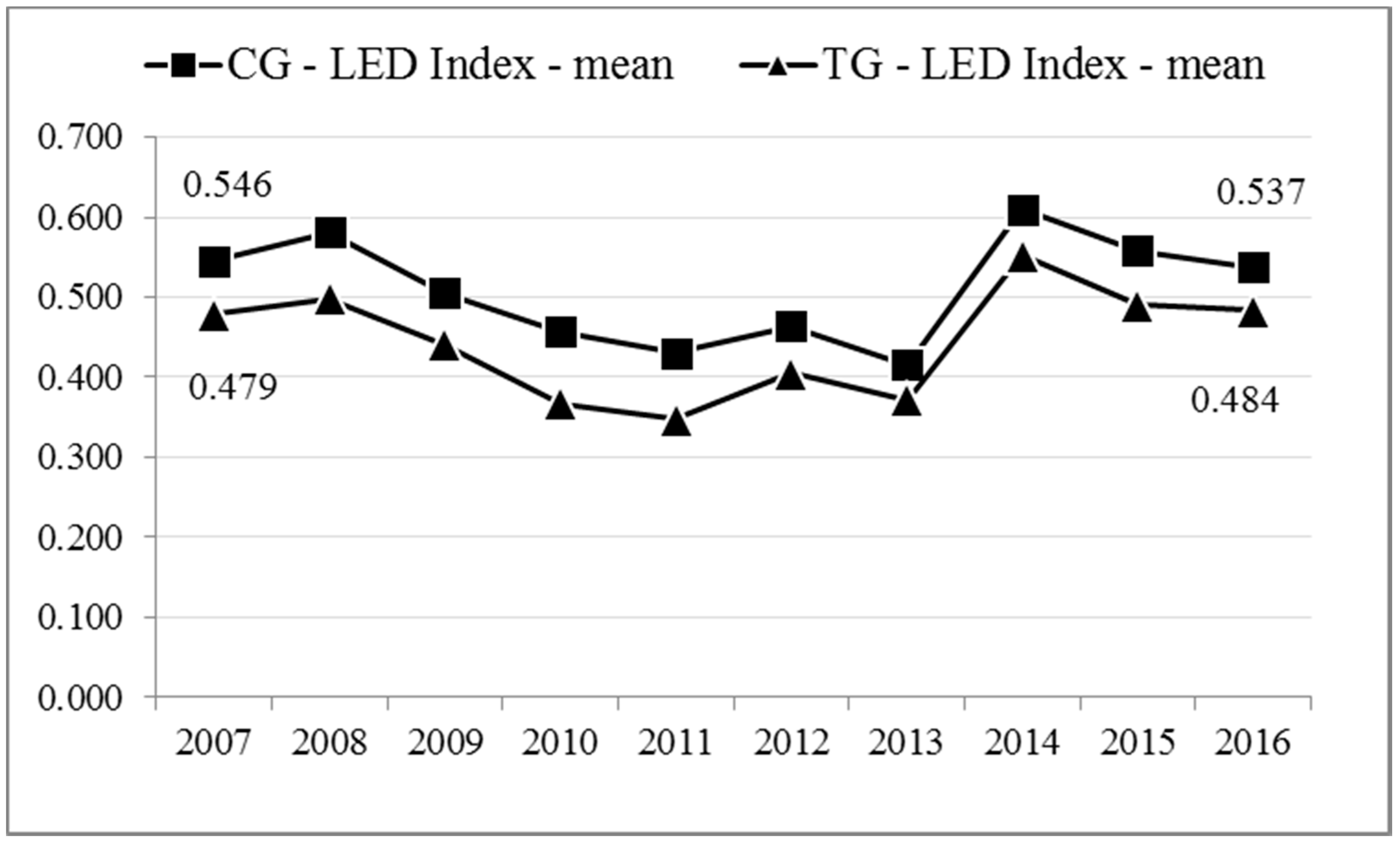
O2 of our research was accomplished through the cvasi-experimental research. As Figure 2 shows, the evolution of LED (mean values of the LED Index) reveals the difference which exists between communes which benefited from infrastructure investments (irrespective of their type) and those which did not during the period 2007–2016.

It is important to observe the initial (2007) difference existing between beneficiaries and non-beneficiaries. This difference is due to the fact that Measure 322 had, as its main goal, to determine a reduction in poverty at local level, coupled with reduction of disparities among rural communities, and therefore, it encouraged the poorest communities to apply. The reason behind this was to counterbalance the trends in EU funds allocation according to which developed regions had better access to European funds, thus widening territorial disparities [75,76]. This was done by giving additional points during the application stage to communities based on their level of poverty. From this perspective, we can say that the goal of poverty reduction succeeded to facilitate the access of the poorest communes to non-refundable programs for basic infrastructure. This is a change compared with other previous European and national non-refundable programs for basic infrastructure in rural communities of Romania, where the beneficiaries were more developed before accessing and implementing the basic infrastructure projects, proving in this case that existing higher level of economic development and higher administrative capacity of the communities facilitated their access to non-refundable programs [52]. Figure 2 also reveals that three years after treatment, the difference between beneficiaries and non-beneficiaries remains somewhat similar. Because differences between 2007 and 2016 are extremely small, graphical representation is supplemented with a comparison of means for the treatment group and the control group. The results are displayed in

Table 3. The evolution of the LED Index, treatment group versus control group.

Groups	LED Index—Mean
	2007	2013	2016	Dif. 2016–2007	2016/2007	Dif. 2013–2007	2013/2007	Dif. 2016–2013	2016/2013	TG/CG 2007	TG/CG 2013	TG/CG 2016
Treatment group (TG)	0.478	0.371	0.483	0.005	1.010	−0.107	0.776	0.112	1.302	0.877	0.894	0.899
Control group (CG)	0.545	0.415	0.537	−0.008	0.985	−0.130	0.761	0.122	1.294

Source: Compiled by the authors.

below.

The annual mean values of the LED Index show an initial development difference between control and treatment group (as displayed by Figure 2), and the fact that the difference was slightly reduced until 2016. Also, it seems that in 2013 (the year of project execution—actual building of works) compared with 2007, the LED Index in the treatment group did not drop as much as in the control group. This is most likely due to spending in the community associated with the presence of workers on the construction sites.

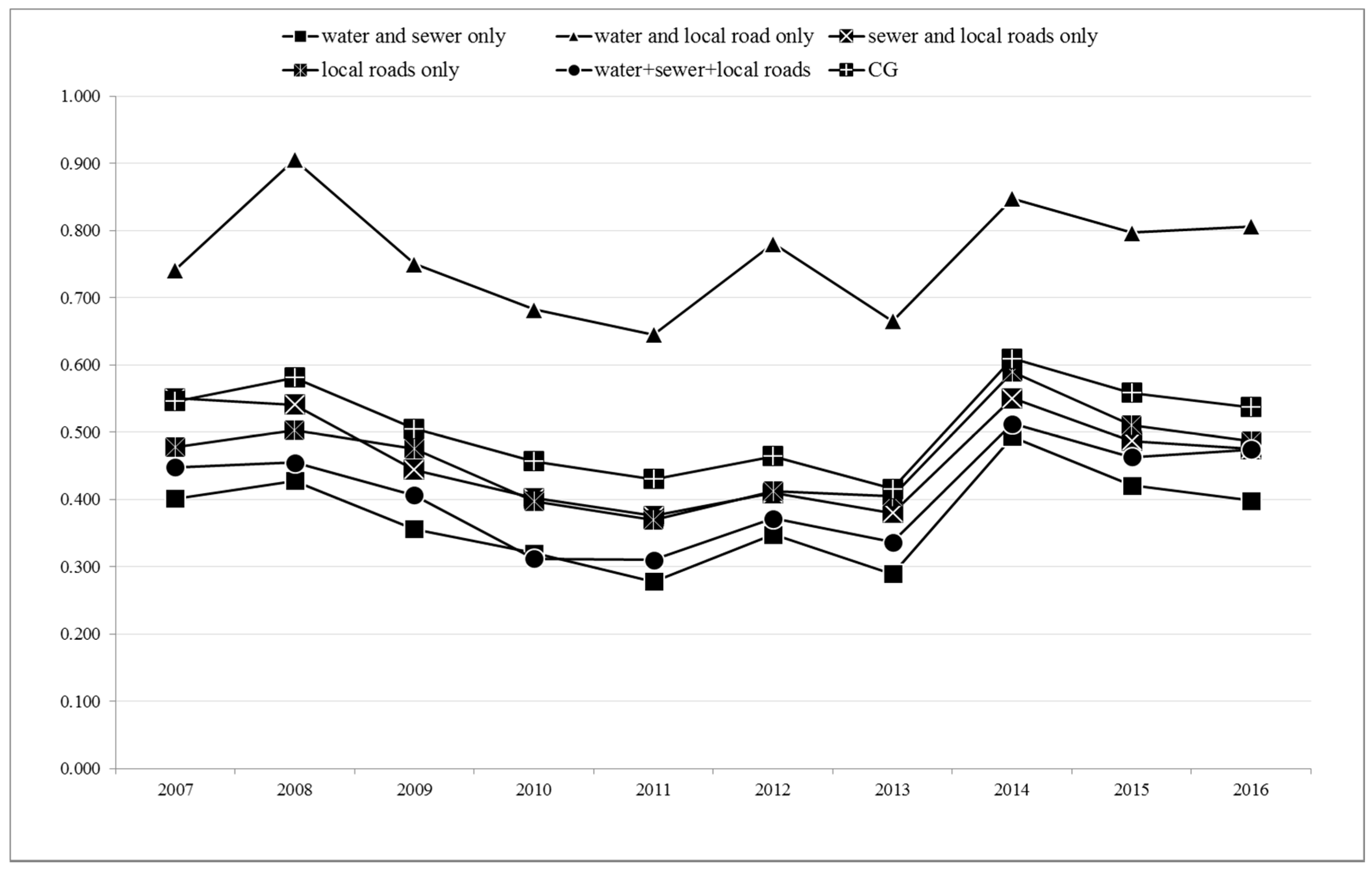
If we break down investments by types of infrastructure, the evolution of the LED Index is portrayed by Figure 3.

The communes which have implemented water and sewage investments (8 cases) started from the lowest level of LED in 2007, while the ones which implemented other combination of investments—sewerage and local roads (9 cases) or water and local roads (3 cases) were at the same level or over the LED Index value compared with the control group. The communes implementing integrated investment projects (containing three type of infrastructure—26 cases) started from the second lowest LED Index level in 2007. Excluding the communes which implemented only water and road projects due to the low number of cases (only 3), it is interesting to observe the evolution of the LED Index over the 2007–2016 period by considering the combination of implemented types of infrastructure investments. The difference between communes in the treatment group and the control group is slightly reduced over 2011–2013 time period (while the projects were executed). After that period, the difference between the treatment and the control group increases until 2016, except for the communes which implemented integrated projects (3 types of infrastructure). Surprisingly, the situation seems to be turned around in 2016 compared to 2007 in the communes implementing water and sewerage projects. In this case, although the average value of LED index was approximately equal with the communes in the control group, from 2009 onward the level decreases, below the value of the control group, including the period of project execution, and the difference increases in the favor of control group starting from 2014.

According to the type of investment implemented, the LED Index mean values in 2007, 2013, and 2016 are presented in

Table 4. Mean LED Index values in 2007, 2013, 2016, according to the type of infrastructure investment.

Category of Investment	LED Index—Mean
	2007	2013	2016	Dif. 2016–2007	2016/2007	Dif. 2013–2007	2013/2007	Dif. 2016–2013	2016/2013	TG/CG 2007	TG/CG 2013	TG/CG 2016
M322- NPRD water + sewerage (8 cases)	0.401	0.289	0.398	−0.003	0.993	−0.112	0.721	0.109	1.377	0.736	0.696	0.741
Control group (CG)	0.545	0.415	0.537	−0.008	0.985	−0.130	0.761	0.122	1.294
M322- NPRD water + local roads only (3 cases)	0.742	0.665	0.806	0.064	1.086	−0.077	0.896	0.141	1.212	1.361	1.602	1.501
Control group (CG)	0.545	0.415	0.537	−0.008	0.985	−0.130	0.761	0.122	1.294
M322- NPRD sewerage + local roads (9 cases)	0.550	0.379	0.475	−0.075	0.864	−0.171	0.689	0.096	1.253	1.009	0.913	0.885
Control group (CG)	0.545	0.415	0.537	−0.008	0.985	−0.130	0.761	0.122	1.294
M322- NPRD local roads (18 cases)	0.477	0.404	0.486	0.009	1.019	−0.073	0.847	0.082	1.203	0.875	0.973	0.905
Control group (CG)	0.545	0.415	0.537	−0.008	0.985	−0.130	0.761	0.122	1.294
M322- NPRD water + sewerage + local roads (26 cases)	0.448	0.336	0.474	0.026	1.058	−0.112	0.750	0.138	1.411	0.822	0.810	0.883
Control group (CG)	0.545	0.415	0.537	−0.008	0.985	−0.130	0.761	0.122	1.294

Source: Compiled by the authors.

.

By comparing the mean values, some observations can be made: (a) In 3 out of the 5 sub-groups of cases in the sample by type of infrastructure investment, the initial LED Index values (2007) are lower than those for the control group; (b) In 4 sub-groups the communes from the treatment group slightly recovered the development gap compared with the control group; (c) Only 3 sub-groups experienced a diminishment in the development gap in 2013, during the execution of the projects.

The next step in the analysis was to assess the difference between beneficiaries and non-beneficiaries before and after the treatment (implementation of the basic infrastructure projects). Using difference-in-differences technique, we applied Mann–Whitney U-test on the value of LED Index for 2007, 2013, 2016 and the difference between treatment group and control group. The results are presented in

Table 5. Mann–Whitney U-test on the values of LED Index for 2007, 2013, 2016, irrespective of infrastructure category.

M 322—NPRD—Not Differentiated Treatment
Year/Difference	Status	N	Mean Rank	Sum of Ranks	Mann–Whitney U	Wilcoxon W	Z	Asym. Sig. (2-Tailed)
2007	Control group	64	66.52	4257.50	1918.500	3998.500	−0.617	0.537
	Treatment group	64	62.48	3998.50
2013	Control group	64	66.61	4263.00	1913.000	3933.000	−0.643	0.520
	Treatment group	64	62.39	3933.00
2016	Control group	64	67.67	4331.00	1845.000	3925.000	−0.967	0.333
	Treatment group	64	61.33	3925.00
LED Index—Difference 2016–2007	Control group	64	62.86	4023.00	1943.000	4023.000	−0.500	0.617
	Treatment group	64	66.14	4233.00
LED Index—Difference 2013–2007	Control group	64	62.78	4018.00	1938.000	4018.000	−0.524	0.600
	Treatment group	64	66.22	4238.00
LED Index—Difference 2016–2013	Control group	64	65.21	4173.50	2002.500	4082.500	−0.217	0.828
	Treatment group	64	63.79	4082.50

Source: Compiled by the authors.

below.

The test shows that in 2007 (before treatment) there is a difference—Mean Rank—but not statistically significant between treatment group and control group. The difference is almost the same in 2013 and 2016 and is not statistically significant as well. Even if the treatment group recovers more than the control group (see the Mean Rank in the case of Index LED—difference 2016–2007), the ‘catching up’ is very small and statistically insignificant. From this perspective, it can be said that, on the short-term (3 years), the investments from Measure 322 in basic infrastructure at local level did not succeed in boosting local economic development. This is not to say that improvements did not occur at the local level—there could be other quality-of-life elements that have improved more significantly at the local level but in the short term the local economy does not seem to have been boosted by infrastructure investments. Quality of life improvements for rural areas of Romania are quite hard to investigate using only statistical data; qualitative techniques should be used in order to capture the true social and well-being impact generated by these projects.

We used the same technique (difference-in-differences) for each indicator aggregated into the LED Index. As expected, for the most part of the indicators there is a difference in favor of the control group, the Mean Rank being higher both in 2007 and 2016. But there are some exceptions. For example, we observed that in the case of income from local taxes per capita, in 2007 (before treatment) there is a difference in favor of the control group, the Mean Rank being higher but not statistically significant in the case of the control group than in the case of the treatment group. In 2016, the situation is changed, the Mean Rank being higher (not statistically significant) in the case of the treatment group. A similar situation is in the case of entrepreneurial capacity, the Mean Rank being higher (not statistically significant) in 2007 in the case of the control group (Mean Rank = 67.00 for the control group and 62.00 for the treatment group) and almost the same for the treatment group and the control group in 2016 (Mean Rank for the control group = 64.52, Mean Rank for the treatment group = 64.48). Also, surprisingly, in the case of number of dwellings completed during the year per 1000 inhabitants, the Mean Rank is higher (but not statistically significant) both in 2007 and 2016 in the case of the treatment group than in the case of the control group: in 2007 Mean Rank for control group = 62.36, Mean Rank for the treatment group = 66.64, in 2016 Mean Rank for the control group = 60.63, Mean Rank for treatment group = 68.38. Based on these results, it is possible that in the short-term (3 years) one immediate and observable impact of investments in basic local infrastructure is the increasing of entrepreneurial capacity, meaning that new companies have been created at the local level. Also, we could speculate that while infrastructure investments do not immediately translate into growth of the local economy, we have other effects at community level, such as willingness and capacity of people to invest in assets such as housing.

A surprising result was obtained in the case of the indicator social assistance expenses (per capita). Even if in 2007 the situation was almost the same in the case of the treatment group and in the case of the control group, in 2016 there is a statistically significant difference between the treatment group and the control group, meaning that social assistance expenses (per capita) are statistically significantly higher in the treatment group than in the control group (see

Table A1. Mann–Whitney U-test on the values of Social assistance expenses (per capita) considering the financing of basic infrastructure through Measure 322, irrespective of the category of investment.

M 322—NPRD—Not Differentiated Treatment
Year/Difference	Status	N	Mean Rank	Sum of Ranks	Mann–Whitney U	Wilcoxon W	Z	Asym. Sig. (2-Tailed)
2007	Control group	64	64.36	41,119.00	2039.000	4119.000	−0.043	0.966
	Treatment group	64	64.64	4137.00
2013	Control group	64	59.30	3795.00	1715.000	3795.000	−1.587	0.113
	Treatment group	64	69.70	4464.00
2016	Control group	64	57.20	3661.00	1581.000	3661.000	−2.226	0.026
	Treatment group	64	71.80	4595.00
Index LED—Difference 2016–2007	Control group	64	59.95	3837.00	175.000	3837.000	−1.387	0.166
	Treatment group	64	69.05	4419.00
Index LED—Difference 2013–2007	Control group	64	62.91	4026.00	1946.000	4026.000	−0.486	0.627
	Treatment group	64	66.09	4230.00
Index LED—Difference 2016–2013	Control group	64	58.09	3718.00	1638.000	3718.000	−1.954	0.051
	Treatment group	64	70.91	4538.00

Source: Compiled by the authors.

). We are hypothesizing that, once the problem of infrastructure is resolved, local authorities have a few more resources to use on other categories of problems, such as social care. Same results were obtained by other authors measuring the impact of other infrastructure programs on the growth of rural economy in Romania [52].

We also investigated if there is a difference between the communes in the treatment group and in the control group, by taking into consideration the category of infrastructure they invested in or the combination of infrastructure categories (see

Table A2. Mann–Whitney U-test on the values of LED Index for 2007–2016 considering the category of local infrastructure financed through Measure 322.

M 322—NPRD—Full Integrated Projects—Water + Sewerage + Local Roads
Year/Difference	Status	N	Mean Rank	Sum of Ranks	Mann–Whitney U	Wilcoxon W	Z	Asym. Sig. (2-Tailed)
2007	Control group	64	39.89	2361.00	231.000	267.000	−0.448	0.654
	Water and Sewerage only	8	33.38	267.00
2013	Control group	64	37.13	2376.00	216.000	252.000	−0.717	0.474
	Water and Sewerage only	8	31.50	252.00
2016	Control group	64	37.34	2390.00	202.000	238.000	−0.968	0.333
	Water and Sewerage only	8	29.75	238.00
Index LED—Difference 2016–2007	Control group	64	36.46	2333.50	253.500	2333.500	−0.045	0.964
	Water and Sewerage only	8	36.81	294.50
Index LED—Difference 2013–2007	Control group	64	36.37	2327.50	247.500	2327.500	−0.152	0.879
	Water and Sewerage only	8	37.56	300.50
Index LED—Difference 2016–2013	Control group	64	36.63	2344.50	247.500	283.500	−0.152	0.879
	Water and Sewerage only	8	35.44	283.50
2007	Control group	64	33.47	2142.00	62.000	2142.000	−1.031	0.303
	Water and local roads only	3	45.33	136.00
2013	Control group	64	33.11	2119.00	39.000	2119.000	−1.728	0.084
	Water and local roads only	3	53.00	159.00
2016	Control group	64	32.95	2109.00	29.000	2109.000	−2.031	0.042
	Water and local roads only	3	56.33	169.00
Index LED—Difference 2016–2007	Control group	64	33.58	2149.00	69.000	2149.000	−0.819	0.413
	Water and local roads only	3	43.00	129.00
Index LED—Difference 2013–2007	Control group	64	33.91	2170.50	90.500	2170.500	−0.167	0.868
	Water and local roads only	3	35.83	107.50
Index LED—Difference 2016–2013	Control group	64	34.13	2184.00	88.000	94.000	−0.243	0.808
	Water and local roads only	3	31.33	94.00
2007	Control group	64	36.34	2325.50	245.500	2325.500	−0.713	0.476
	Sewerage and local roads only	9	41.72	375.50
2013	Control group	64	36.68	2347.50	267.500	2347.500	−0.344	0.731
	Sewerage and local roads only	9	39.28	353.50
2016	Control group	64	37.05	2371.50	284.5000	329.500	−0.059	0.953
	Sewerage and local roads only	9	36.61	329.50
Index LED—Difference 2016–2007	Control group	64	37.91	2426.50	229.500	274.500	−0.982	0.326
	Sewerage and local roads only	9	30.50	274.50
Index LED—Difference 2013–2007	Control group	64	37.89	2425.00	231.000	276.000	−0.956	0.339
	Sewerage and local roads only	9	30.67	276.00
Index LED—Difference 2016–2013	Control group	64	37.31	2388.00	268.000	313.000	−0.336	0.737
	Sewerage and local roads only	9	34.78	313.00
2007	Control group	64	43.28	2770.00	462.000	633.000	−1.277	0.202
	Local roads only	18	35.17	633.00
2013	Control group	64	43.01	2752.50	479.500	650.500	−1.081	0.280
	Local roads only	18	36.14	650.50
2016	Control group	64	44.03	2818.00	414.000	585.000	−1.815	0.070
	Local roads only	18	32.50	585.00
Index LED—Difference 2016–2007	Control group	64	41.02	2625.50	545.500	2625.500	−0.342	0.733
	Local roads only	18	43.19	777.50
Index LED—Difference 2013–2007	Control group	64	40.17	2571.00	491.000	2571.000	−0.952	0.341
	Local roads only	18	46.22	832.00
Index LED—Difference 2016–2013	Control group	64	43.26	2768.50	463.500	634.500	−1.260	0.208
	Local roads only	18	35.25	634.50
2007	Control group	64	46.55	2979.00	765.000	1116.000	−0.596	0.551
	Water + sewerage + local roads	26	42.92	116.00
2013	Control group	64	46.69	2988.00	756.000	1107.000	−0.677	0.499
	Water + sewerage + local roads	26	42.58	1107.00
2016	Control group	64	46.29	2962.50	781.500	1132.500	−0.450	0.653
	Water + sewerage + local roads	26	43.55	1132.50
Index LED—Difference 2016–2007	Control group	64	43.88	2808.50	728.500	2808.500	−0.921	0.357
	Water + sewerage + local roads	26	49.48	1286.50
Index LED—Difference 2013–2007	Control group	64	44.44	2844.00	764.000	2844.000	−0.605	0.545
	Water + sewerage + local roads	26	48.12	1251.00
Index LED—Difference 2016–2013	Control group	64	43.88	2808.50	728.500	2808.500	−0.921	0.357

Source: Compiled by the authors.

). First of all, we have to mention that the differences are not statistically significant, with the exception of water + local roads category, in 2016, but this is a particular situation due to the low number of cases. The Mann–Whitney U-Test reveals similar results with those obtained from comparing the means, with some exceptions. 3 out of 5 sub-groups in the treatment group reduced the development gap compared to the control group over the period 2007–2013; after 2013, 2 sub-groups lost again the advantage gained during the course of the previous period. These results are in line with our hypothesis that at least in some cases, the actual execution of construction works offered an extra boost for the local economy. An important observation is that the communes which implemented integrated investment (water + sewerage + local roads) seem to recover continuously the difference existing between them and the control group, irrespective of pre-treatment and post treatment period (2007–2016), implementation period (2007–2013), or post implementation period (2013–2016). This seems to suggest that the view according to which one type of infrastructure (roads) is more important than other types, is not valid.

O3 of our research deals with identifying possible determinants for LED, other than public investments in infrastructure. We used several linear regression models for achieving this objective. In the first regression model, we included four independent variables. For the level of LED, the dependent variable, we used the mean of LED Index during 2007–2016 period. The model only shows, in general, which independent variable influences the level of economic development as approximated by the LED we constructed. The results are presented in

Table 6. Determinants for LED in the control + treatment groups.

Model Summary	R	R Square	Adj R Square	Std. Error	Sig. F Change	Durbin-Watson
	0.791	0.626	0.614	0.242	0.000	1.980
Dependent variable: The level of LED (LED Index—mean for 2007–2016 period)
Coefficients	Independent Variables		B	Std. Error	Beta	t	Sig
	Direct connection to the European road network		0.150	0.050	0.169	2.988	0.003
	Direct connection to the national roads network		0.115	0.054	0.121	2.143	0.034
	Population size		0.050	0.020	0.148	2.581	0.011
	Percentage of university graduates		10.477	0.907	0.664	11.554	0.000

Source: Compiled by the authors.

.

R² indicates that the explanatory power of the model is medium to strong, as the independent variables together explain 62.6% of the variation of the arithmetic mean of the LED Index. The main statistically significant determinants of LED are the percentage of university graduates (educational stock in the community) (0.664 ***) and direct connection to the European road network (0.169 ***), while population size and direct connection to the national road network are the weakest predictors. It is not surprising that the presence of educated population in a rural community acts as a determinant for LED. Given the fact that our constructed LED Index focuses mostly on economic/market indicators, we expected to see an influence of education at community level on the number of new firms created, number of employees, revenues obtained from company income tax, etc. Education level matters in the context of rural communities not only when it comes to the entrepreneur themselves but also the labor force available in those communities [77]. Given that most communities in the sample are rather remote, entrepreneurs creating businesses here have to rely, for the most part, on local work force. We strongly believe that the connection to national or European roads and size of the community matter. However, the low explanatory power of these variables in our study could be due to the sample investigated. Both the control and treatment group include a majority of communities which are rank 1—this means they are remote from urban centers and in certain cases, rather small. This is why perhaps the explanatory power of these variables is low. It has to be further investigated if the same results will be obtained for a larger sample, equally stratified based on the rank of the rural commune.

A second regression model was developed, in this case, the dependent variable been the LED Index measured as difference between 2016 and 2007. This second dependent variable is different from the first one in that it captures the boosting effect of the local economy by certain factors. We employed the same independent variables as in the first regression model, plus public investments in local basic infrastructure financed through Measure 322. The latter variable was included as treatment added during the period 2007–2016. The rest of the independent variables are relatively stable over long periods of time, and changes in them can only occur as result of various reforms and policies implemented by central government (for example significant changes in size of population is expected to happen in rural areas only through amalgamation). Our expectation was to observe a boosting effect of the local economy in relation to investments in basic infrastructure; also, we expected to see that the education stock in the community, the variable with the highest explanatory value in the previous model, also acts as a boosting factor for LED.

The explanatory power of the model is low, as the independent variables explain only 8.6% of the variation of the LED Index difference between 2007 and 2016 (please see

Table 7. Determinants for boosting LED in the control + treatment groups.

Model Summary	R	R Square	Adj R Square	Std. Error	Sig. F Change	Durbin-Watson
	0.293	0.086	0.049	0.203	0.049	2.194
Dependent variable: LED Index difference: 2016–2007
Coefficients	Independent Variables		B	Std. Error	Beta	t	Sig
	Direct connection to the European road network		−0.009	0.042	−0.018	−0.204	0.839
	Direct connection to the national road network		0.018	0.045	0.035	0.394	0.694
	Population size		−0.053	0.017	−0.290	−3.205	0.002
	Percentage of university graduates		−0.121	0.780	−0.014	−0.155	0.877
	M 322—NPRD		0.016	0.037	0.038	0.421	0.675

Source: Compiled by the authors.

). This means that while the LED level is susceptible to be influenced by community characteristics such as remoteness, size, and education stock, variations in LED Index are harder to predict and explain. The factors usually described in the literature as determinants of administrative capacity for Romanian rural communities seem to play no role in LED variations over time. Moreover, for certain determinants we obtained that they are negatively (and statistically significant) correlated with the LED Index evolution. On the short and medium term, investments in local infrastructure ranging from 1–6 million euros have little effect on the local economy (measured especially in terms of market indicators). In light of these findings, it could be argued that local economy is perhaps more prone to being influenced by policies at the national level and by the general economic climate.

5. Conclusions

Romania lags severely behind other EU countries in terms of infrastructure endowment and the belief of both lay people and decision-makers is that infrastructure investments represent the magic wand towards national prosperity. National and EU funded programs addressing the infrastructure gap, especially in rural areas, are implemented with three declared objectives in mind—grow the local economy, reduce poverty, and generate increased quality of life for the rural residents. Our study focused on the impact of infrastructure investments on the local rural economy. H1 of our study, therefore, tried to verify if rural communes which implemented infrastructure projects financed from Measure 322 have developed faster than the ones which did not access funds through this program. This hypothesis is only partially confirmed. The beneficiaries of Measure 322 have developed somewhat more, but not statistically significant more so than those who have not benefited from this program. Some specific indicators, which were used to the construction of LED Index, such as entrepreneurial activity and budgetary revenue from local taxes, increased more in the communes benefiting from infrastructure investments, but this increase is not statistically significant. More surprising is that social assistance expenses (per capita) are statistically significantly higher in the communes which received financing than in those which did not, even if in 2007 (pre-treatment) they were at the same level for both groups (beneficiaries and non-beneficiaries). The results of our research do not mean necessarily that these projects will not generate significant economic impacts later on. The research investigated projects completed in 2013, and it is possible that the interval 2013–2016 is too short for observing significant changes in the local economy. Some of the studies outlined in Section 2 found these effects are more than 10 years from the completion of the works. The results of our study are in line with the research by the authors of [78], who found that in the short term (up to 10 years) there is no observable positive effect of introducing and modernizing water and sewage systems in rural communities from Oklahoma. Instead, the study observes a positive, and statistically significant effect on the average value of houses in the localities that benefited from the funding program—an increase between 5% and 13% of the median of average house prices. This seems to suggest that an LED Index built mainly on market indicators is less useful towards investigating short and medium terms impact of publicly funded infrastructure program. However, the additional challenge in Romania is to find available data at the level of rural communities which measure more relevant indicators for LED other than the ones used in this study.

H2 tried to assess one specific feature of Measure 322, namely integrated infrastructure investments. With this program, government authorities argued that it is better to pursue all types of infrastructure at once, in order to see accelerated growth at the local level. H2 stated that rural communities implementing integrated infrastructure projects (water + sewerage + local roads) developed at a faster pace than those which have not accessed funding through the program, or have implemented investment projects with only one or two components. H2 is also only partially confirmed. The communes which implemented integrated project have developed constantly over the monitored interval and a little bit more, but not statistically significant than those which did not benefited from Measure 322.

One assumption of our research, incorporated in H3, was that during the execution/construction phase of local basic infrastructure projects the local economy of communes grows at a higher pace, compared to that of communes which have not benefited from funding. We expected this impact to occur because construction means more people/workers on site, more resources for consumption in the local community, and perhaps even more economic activity in the form of local firms providing some materials or workforce. H3 is only partially confirmed. During the execution phase, the local economy of beneficiaries grows at a higher pace but not statistically significant compared with that of non-beneficiaries. Moreover, if we look at the category of infrastructure communes invested in, we observe that in the case of sewerage and local roads category of investment, the situation is the opposite.

In our research, we were also interested in what factors act as determinants of local economic development. We mainly investigated features connected with the local communities in the sample. This was done, mindful of the fact that when decision-makers create the list of criteria based on which projects are awarded, they have the possibility to encourage communities having certain features to apply. Knowing what characteristics favor LED can be important for how future programs are structured. With H4, we decided to observe if certain characteristics of the local communes have an impact of local economic development. Thus, we hypothesized that the size of the commune’s population, direct access to European and national road networks, and percentage of university graduates in total population (education stock) act as predictors of LED. H4 is confirmed, the main statistically significant predictors for LED being the percentage of university graduates in the total population of the community and direct connection to a European road network. Similar results were obtained by the authors of [62] in 1995—their study confirms a relationship between highway connection of small communities in Iowa, US and their economic development; it also confirmed the existence of a relation between the location of the community, human capital and economic development of said communities. Another important conclusion is that none of the predictors for the level of LED are not statistically significant predictors for boosting LED. The situation is similar in the case of non-refundable investment projects in local basic infrastructure, no matter the category of investment (integrated or both or only one component of infrastructure) is not a statistically significant predictor for boosting LED.

The results of our study can at least tentatively indicate several aspects which need to be considered by policy-makers when designing publicly financed programs which target LED in rural areas:

Measure 322 for the first time encouraged the poorest communities in the rural areas to apply, through the use of specific eligibility and selection criteria. Under similar programs financed from EU or national funds, the poorest communities did not have a chance of being successful in a project competition due to limited administrative capacity (capacity to write the grant proposal, to co-finance it, to implement it, etc.). While the intention of M 322 is laudable, it does come at a cost. More than 55% of the projects financed through Measure 322 were not completed 5–6 years after the signing of the contract. Some of them are still pending even in 2018. Decision-makers should consider in the future not only to facilitate the application of the poorest communities to these grants but also to offer them technical assistance during implementation. Measure 322 for example encouraged communities to partner for implementing some projects under the assumption that partnerships will counteract the limited administrative capacity. However, partnerships proved difficult to handle in the absence of prior experience in this area.

The objectives followed by national and EU decision-makers in connection to investment programs in basic infrastructure need to be more nuanced. Thus, if the main objective is to facilitate the access of rural residents to basic services, LED can only be a distant objective, to be achieved at best on the long run and only if certain perquisites are met: rural communities are situated in the close proximity of urban centers, local population is educated and qualified, accessibility and connectivity are good, etc. On the other hand, if access and increasing living conditions is desired, then stronger penalties need to be included in the contracts for the non-use of the built infrastructure. Two situations are commonly occurring in rural areas: first, residents refuse to connect to sewage and water because the user fees are high and the infrastructure is not used; second, local communities after completion of the project do not have proper resources to ensure adequate maintenance of the built infrastructure.

Projects targeting integrated investments in all types of basic infrastructure should be preferred over those which only support one type of infrastructure. At national level, investments in roads are seen as the first priority. However, it becomes clearer, though, despite roads being a prerequisite, water and sewage are also required for economic operators. For production facilities, sewage and water are essential, not only due to the requirements of production, but also due to authorization procedures, which include very stringent environmental rules.

The strong relation between LED in rural communities and education stock of the population may be an argument for the national decision-makers to intensify measures and strategies aimed at preventing school dropout in rural areas and encouraging students to apply for higher education programs. Some recent measures taken in the area of higher education seem to suggest that attraction and retention of university graduates in rural areas is of importance for the national government. On the other hand, local authorities should also understand that attraction and retention of educated population should be a priority if they want to see some results in terms of economic development and entrepreneurship.

This research has several major limitations which need to be acknowledged. First, the impact of investments is measured after a very short period of time, 3 years, since the completion of the projects. While some effects, such as the increase in entrepreneurial capacity take place rather soon, others might not occur for another decade. Second, the variable infrastructure investment is measured in a dichotomic manner, whether communes benefited or not from the investments. This means that we are treating all investments in a certain category as similar, which is not the case in reality. While the value of the projects is more or less comparable, the actual results in terms of kilometers of roads or water or sewage built varies a lot. These data are not currently accessible and this is the reason why, for the purpose of this study, investments were accounted for in communities with yes or no. Third, we assumed in the research that all communities which finalized the infrastructure projects starting to reap the benefits of better infrastructure. However, this is not the case because it is impossible to know if the residents actually use the sewage and water infrastructure and what is the percentage of users in the total population of a given community. Fourth, there are no data in place regarding other investments made at local level in basic infrastructure during the same period of time from the local budget (own resources). If significant investments are made from own resources, especially in the wealthier communities, these could also explain why the development gap persists even after measure 322 had been implemented.