Uncertainty Analysis for the CH4 Emission Factor of Thermal Power Plant by Monte Carlo Simulation


1
Climate Chang Research Center, Sejong University, Seoul 05006, Korea
2
Department of Environment & Energy, Sejong University, Seoul 05006, Korea
*
Author to whom correspondence should be addressed.
Sustainability 2018, 10(10), 3448; https://doi.org/10.3390/su10103448
Submission received: 29 August 2018
/
Revised: 21 September 2018
/
Accepted: 25 September 2018
/
Published: 27 September 2018
(This article belongs to the Special Issue Circular Economy—Sustainable Energy and Waste Policies)
Abstract
:Thermal power plants are a large source of greenhouse gas emissions among energy industry facilities. Emission factors for methane and nitrous oxide depend on combustion technologies and operating conditions and vary significantly with individual thermal power plants. Due to this variability, use of average emission factors for these gases will introduce relatively large uncertainties. This study determined the CH4 emission factors of thermal power plants currently in operation in Korea by conducting field investigations according to fuel type and type of combustion technique. Through use of the Monte Carlo simulation, the uncertainty range for the CH4 emission factor was determined. The estimation showed, at the 95% confidence level, that the uncertainty range for CH4 emission factor from a tangential firing boiler using bituminous coal was −46.6% to +145.2%. The range for the opposed wall-firing boiler was −25.3% to +70.9%. The range for the tangential firing boiler using fuel oil was −39.0% to 93.5%, that from the opposed wall-firing boiler was −47.7% to +201.1%, and that from the internal combustion engine boiler was −38.7% to +106.1%. Finally, the uncertainty range for the CH4 emission factor from the combined cycle boiler using LNG was −90% to +326%.
1. Introduction
With the acceptance of the Paris Agreement on 12 December 2015, at the Paris 2015 UN Climate Change Conference, an ambition to limit global warming to no more than 1.5 °C above pre-industrial levels has been stated and a growing emphasis has been placed on the need to improve the statistical reliability of national greenhouse gas inventories [1,2,3]. The main ideas of the Paris Agreement are that (i) all participating nations of the UN Framework Convention on Climate Change should join together in developing greenhouse gas removal plans and (ii) should submit an updated report of Intended Nationally Determined Contributions (INDC) every five years based on the principle of progression in preparation for the five-year Global Stocktake. The section on the Global Stocktake, in particular, states, “The Conference of Parties (COP) will conduct the first Global Stocktake in 2023, and unless the COP of the Paris Agreement states otherwise, subsequent Stocktakes will take place every five years”. [4] To prepare for the five-year Global Stocktake, it is critical to improve the reliability of greenhouse gas inventories, which may begin with understanding the emission factor uncertainty essential for estimating greenhouse gas emission. The purpose of uncertainty analysis for greenhouse gas inventories is to enable more accurate and precise estimation of greenhouse gas emission. The main sources of uncertainty in greenhouse gas emissions are the lack of knowledge of emission factors and activity data [5].
Uncertainties of greenhouse gas inventory are defined as the “lack of knowledge of the true value of a variable that can be described as a probability density function (PDF) characterizing the range and likelihood of possible values [6]”. For analyzing such uncertainties, Volume 1, Chapter 3, of the 2006 IPCC Guidelines provides guidance for estimating and reporting uncertainties associated with annual estimates of emissions and removals and emission and removal trends over time. Two approaches are suggested for combining uncertainties. Approach 1 employs certain key assumptions to simplify the calculations, providing relatively simple, spreadsheet-based procedures. Approach 2 employs the Monte Carlo simulation. Whereas Approach 1, based on error propagation, can be applied to cases with a relatively small range of uncertainties where the standard deviation divided by the mean is less than 0.3, in theory, Approach 2, based on the Monte Carlo simulation, is suitable for cases in which uncertainties are large or the distribution is non-normal [7].
This study aims to determine the uncertainties in CH4 emission factors at thermal power plants in Korea. Emissions of greenhouse gases from Korea account for the highest percentage of CO2 emissions (92%) and CH4 emissions account for approximately 4%, which is the highest percentage of non-CO2 greenhouse gases. Therefore, taking into account the share of GHG emissions, CH4 emissions cannot be ignored in the total GHG emissions or inventory confidence.
Also, consider the 100-year time horizon Global Warming Potentials (GWPs) from the Intergovernmental Panel on Climate Change (IPCC) forth Assessment Report, CH4 has a very high contribution of approximately 25 times that of CO2 and accurate CH4 emission estimates are needed.
CO2 emission in the power generation sector is dependent on the fuel carbon fraction, and if the precise mechanism by which the fuel carbon combines with O2 during combustion to produce CO2 is known [8]. On the contrary, the production of CH4 has not been defined clearly, and the characteristics of CH4 emission vary according to diverse factors such as fuel type, fuel carbon and nitrogen fractions, combustion conditions, and air pollution control equipment [9]. Additionally, the 2006 IPCC Guidelines suggest default uncertainty estimates for the emission factors, and in the power generation sector, the default uncertainty range for the CH4 emission factor is 50–150%, which is far higher than the 7% uncertainty for the CO2 emission factor. Thus, the uncertainties in CH4 emission factor at thermal power plants were determined through Approach 2 based on the Monte Carlo simulation [10].
For this determination, the CH4 concentration of exhaust gas was analyzed by carrying out field investigations at three power plants in Korea that use bituminous coal as fuel, and based on the fuel analysis results, including the heat generation rate and elemental analysis provided by the power plants, the CH4 emission factor was determined. Then, the Monte Carlo simulation was used to determine the uncertainties in the CH4 emission factor.
2. Materials and Methods
2.1. Designation of Subject Facilities and Sampling Period
The subject thermal power plants in this study were three power plants using bituminous coal as fuel, three power plants using bunker fuel oil, and one power plant using liquefied natural gas. Table 1 summarizes the installed capacity, fuel consumption, fuel type, and boiler type of the subject thermal power plants. At each power plant, three field investigations over three days were performed.
2.2. Exhaust Gas Sampling Method
To determine the CH4 emission factor at a power plant, field investigations for the exhaust gas discharge, temperature, and water content; gas sample analyses are also essential. Thus, during greenhouse gas sampling in the field, exhaust gas temperature, water content, air temperature, flow rate, and pressure were measured [11,12].
Because the exhaust gas temperature at a greenhouse gas emission facility is generally around 100 °C or higher, the gas sampling tube or pipe should be made of a material that can endure high temperature and flow rate. Thus, in this study, gas sampling tubes made of stainless steel material that can withstand high temperature and exhaust gas flow rate were prepared according to the Standard Methods for the Measurement of Air Pollution in Korea (minor diameter 7 mm). The tube length was 1.5 m. For use in large minor diameters or the inner walls of a stack, two tubes were connected.
To remove the moisture in the exhaust gas and thus prevent it from mixing with the greenhouse gas sample, a gas absorption bottle containing silica gels was installed at the front portion of the exhaust gas collecting device. To prevent moisture condensation that could clog the filter medium and cause corrosion of the tube or conduit, the entire length of the sampling tube was heated to around 120 °C by electric heating and silica gels were used to scavenge moisture from the exhaust gas.
2.3. Analysis Method of CH4 Concentration
Gas chromatography with flame ionization detection (GC-FID) was used to analyze the concentration of CH4 emission at the power plants. The column used for the CH4 analysis was the Porapak Q 80/100, the discharge of both the carrier gas and hydrogen gas was 30 mL/min, and the discharge of air was set at 300 mL/min. The temperatures were set as 100 °C for the injector, 80 °C for the oven, and 250 °C for the detector. Ultrapure nitrogen (99.999%) was used as the carrier gas. The GC-FID analysis conditions for CH4 analysis are presented in Table 2.
To analyze the greenhouse gas, the calibration curve of the target substance prior to analysis was constructed and used to estimate the emission concentration. Standard gas at 1.1 ppm, 3.02 ppm, 5.0 ppm, and 10.0 ppm was used to draw the calibration curve of CH4. As shown in Figure 2, the calibration curve showed excellent linearity with R2 = 0.9998.
The lower limit of detection (LLD) refers to the minimum detectable amount of a given substance that does not have to be quantified. In general, the LLD is differentiated into the instrument detection limit (IDL), when the sample is injected directly to the analytical instrument, and the method detection limit (MDL), when pretreatment or analysis is involved. The LLD can be estimated using (i) a method based on visual inspection; (ii) a method based on signal-to-noise ratio; or (iii) a method based on standard deviation and the gradient of the calibration curve [14].
For the LLD in this study, at least seven samples that displayed a detectable emission concentration of the target gas were analyzed. As shown by Equations (1)–(3), the standard deviation for each sample was multiplied by the t-distribution value of 3.143 within n − 1 degrees of freedom (a value corresponding to 6 degrees of freedom at the 98% confidence level) [15]. Such a concept of MDL is employed by EPA departments and testing agencies as well as many different testing methods, including those published by the American Public Health Association, American Water Works Association, and American Society for Testing and Materials (ASTM) International.
Here, Xi is the ith test value for variable x, X is the mean value for x measured n times, and MDL is the method detection limit (lower limit of detection).
To determine the MDL, standard CH4 gas of 1.00 ppm was used and each analysis was repeated seven times. As the results in Table 3 show, the MDL for CH4 was 10.61 ppb. Within the exhaust gas at power plants reported in previous studies CH4 emission concentration exceeded 0.1 ppm [16,17,18], suggesting that the MDL is suitable for measuring the CH4 emission concentration within the exhaust gas at the power plants.
2.4. Calculation Method of CH4 Emission Factor
The CH4 production from fuel combustion in a stationary emission source results from incomplete combustion, and in such cases, CH4 production is influenced greatly by the operating conditions of the facility. Thus, prediction of CH4 emission based on the general combustion reaction is not possible, and for its estimation, the fuel gas and CH4 concentrations from the combustion at the emission source should be measured.
In large-scale combustion facilities, in particular, measuring the combustion fuel gas concentration requires advanced technology and equipment, so in most cases, fuel combustion properties (values from elemental analysis) are used to derive the combustion reaction and calculate the theoretical concentration of the fuel gas used for estimating the emission factor. This method is already in application in advanced countries such as Japan and the United States. Especially in Japan, the method is used for estimating the emission factor related to non-CO2 emissions from a stationary source [19]. Thus, to estimate the emission factor in this study, the measured gas composition, calculated fuel gas concentration, and theoretical air concentration were fed into an equation such as Equation (4). Here, the net calorific value of each combustion fuel was obtained from the values from the analysis at the power plants. The air ratio, m, was calculated approximately using the O2 concentration within the exhaust gas and the equation below:
m = Air ratio = actual air volume/theoretical air volume (-)
MW = Molecular weight of CH4(constant) = 16 (g/mol)
Vm = One mole ideal gas volume in standardized condition (constant) = 22.4 (10−3 m3/mol)
NCV = Net calorific value for each fuel combustion (MJ/original unit)
However, the air ratio “m” is approximately provided with O2 concentration in exhaust gas, as shown in the equation below
= O2 concentration in exhaust gas (%)
2.5. Goodness-of-Fit Test of Probability Density Function
The Monte Carlo simulation requires that PDFs be specified, where they reasonably represent each model input for which the uncertainty is quantified. For this, a goodness-of-fit test of PDF was carried out.
Goodness-of-fit is a statistical method of inference used to determine whether the distribution of given samples (data) follows the theoretical distribution. The null hypothesis of a test is that the distribution of the samples follows the estimated theoretical distribution, and rejecting it indicates nonconformity to the theoretical distribution. Rejection of the null hypothesis is determined by the significance level α. When the p-value calculated from the test statistic is less than α, rejection occurs.
The test statistics used for the goodness-of-fit test in this study were the K–S statistic and the A–D statistic. The K–S statistic is a test using the statistic D based on an empirical distribution, and D is calculated as shown in Equation (5) below.
where, Y1, Y2, …, YN: N ordered data point.
F: The theoretical cumulative distribution.
An advantage of the K–S test is that D remains uninfluenced by the cumulative distribution function of the theoretical distribution to be tested, so the test is a type of exact test. On the other hand, the test has a tendency to be more sensitive in the middle than in the tails of the distribution, and the circumstance that all parameters of the distribution should be defined poses a limitation.
The A–D statistic can be applied to certain distributions for which the limitation of the K–S statistic becomes problematic because the test places more weight on the tail of the distribution than does the K–S statistic. The test statistic A2 is calculated by Equation (6):
where, .
Y1, Y2, …, YN: N ordered data points.
F: The theoretical cumulative distribution.
2.6. Uncertainty Analysis by Monte Carlo Simulation
To determine the uncertainties of the greenhouse gas emission factor, the Monte Carlo simulation was applied through the four steps illustrated in Figure 3. The first step specifies the model and composes the worksheet for estimating the greenhouse gas emission factor. The second step uses the goodness-of-fit test to verify the PDFs for the input variables related to the greenhouse gas emission factor. The significance level for the hypothesis testing was 5%. Through the goodness-of-fit test, the PDF of each set of data required for estimating the CH4 emission factor, including CH4 emission concentration, discharge, fuel consumption, and the low heating value of the fuel, was evaluated. The Monte Carlo simulation is carried out in the third step: a “Crystal ball” is used to perform random sampling simulations. In the fourth step, the result of the simulation is used to determine the range of uncertainties based on the 95% confidence interval.
3. Result and Discussion
3.1. Exhaust Gas Analysis and CH4 Emission Factor
Among the exhaust gases at the subject facilities, the CH4 concentration and the CH4 emission factors were estimated based on the concentrations presented in Table 4. In plant A, running a tangential firing boiler using bituminous coal, the mean CH4 concentration was 0.51 ppm, with a standard deviation (SD) of 0.18 ppm and relative SD (RSD) of 35.4%. Among the exhaust gases, the mean O2 concentration was 5.62%, and based on this, the average CH4 emission factor was calculated as 0.14 kg CH4/TJ (SD = 0.05, RSD = 33.3%). In plant B, using the same type of fuel and boiler as plant A, the mean CH4 concentration was 0.54 ppm, with SD of 0.38 ppm and RSD of 71.7%. The mean O2 concentration was 5.25%, and based on this, the average CH4 emission factor was calculated as 0.15 kg CH4/TJ (SD = 0.11, RSD = 73.1%). The findings indicated similar CH4 emission factors from plants A and B as they used the same type of fuel and incineration facilities.
On the contrary, in plant C, where an opposed wall-firing boiler using bituminous coal was run, the mean CH4 concentration was 0.30 ppm, with SD of 0.07 ppm and RSD of 22.1%. The mean O2 concentration was 3.89%, and the average CH4 emission factor was estimated as 0.08 kg CH4/TJ (SD = 0.02, RSD = 20.7%), indicating an approximately 47% lower level of emission than from the tangential firing boilers using bituminous coal, whose CH4 emission factors were 0.14 kg CH4/TJ and 0.15 kg CH4/TJ, respectively. The findings confirmed that CH4 emission factors may differ according to the type of combustion despite the use of an identical type of fuel.
In plant D, running an opposed wall-firing boiler using fuel oil, the mean CH4 concentration was 0.69 ppm, with SD of 0.37 ppm and RSD of 54%. The mean O2 concentration was 5.89%, and based on this value, the CH4 emission factor was calculated as 0.17 kg CH4/TJ (SD = 0.02, RSD = 20.7%). In plant E, running a tangential firing boiler using fuel oil, the mean CH4 concentration was 0.48 ppm, with SD of 0.13 ppm and RSD of 27.9%. The mean O2 concentration was 5.81%, and the average CH4 emission factor was 0.12 kg CH4/TJ (SD = 0.02, RSD = 20.7%).
In plant F, running an internal combustion engine using fuel oil, the mean CH4 concentration was 1.03 ppm, with SD of 0.26 ppm and RSD of 25.4%. The mean O2 concentration was 14.38%, and the average CH4 emission factor was 0.61 kg CH4/TJ (SD = 0.02, RSD = 20.7%). This was approximately four times higher than the CH4 emission factors of the tangential firing and opposed wall-firing boilers using fuel oil.
In plant G, running a combined cycle boiler using LNG, the mean CH4 concentration in the exhaust gas was 0.11 ppm, with SD of 0.08 ppm and RSD of 76.9%. The mean O2 concentration was 13.7%, and the calculated average CH4 emission factor was 0.05 kg CH4/TJ (SD = 0.02, RSD = 20.7%).
Among the CH4 emission factors at the thermal power plants using bituminous coal, fuel oil, or LNG, the lowest estimated emission factor was obtained from the thermal power plants using LNG. The thermal power plants use fuel oil, except for the one plant running an internal combustion engine, and all of the thermal power plants using bituminous coal had similar levels of emission factor.
3.2. Monte Carlo Simulation
The Monte Carlo simulation results for the thermal power plants according to fuel type and boiler type are presented in Figure 4. In the simulation of CH4 emission factor from the tangential firing boiler using bituminous coal, the PDF for the CH4 emission factor showed a lognormal distribution with a long tail on the right that was skewed toward the left (skewness = 3.18). The mean was 0.143 kg CH4/TJ, and the median was 0.124 kg CH4/TJ. At the 95% confidence level, the lower 2.5% level was 0.078 kg CH4/TJ and the upper 97.5% level was 0.345 kg CH4/TJ. The PDF for CH4 emission factor from the opposed wall-firing boiler showed a lognormal distribution with a long tail on the right that was skewed toward the left (skewness = 2.68). The mean was 0.079 kg CH4/TJ, the median was 0.074 kg CH4/TJ, and at the 95% confidence level, the lower 2.5% level was 0.059 kg CH4/TJ and the upper 97.5% level was 0.135 kg CH4/TJ.
For the boilers using fuel oil, simulations were carried out according to the type of combustion: tangential firing, opposed wall-firing, or internal combustion engine. In the simulation of the CH4 emission factor from the tangential firing boiler using fuel oil, although the PDF for the CH4 emission factor showed a lognormal distribution with a long tail on the right that was skewed toward the left (skewness = 0.002), it was apparent that the distribution was close to the normal distribution. The mean CH4 emission factor was 0.124 kg CH4/TJ, and the median value was 0.114 kg CH4/TJ. At the 95% confidence level, the lower 2.5% level was 0.075 kg CH4/TJ and the upper 97.5% level was 0.247 kg CH4/TJ. The PDF for CH4 emission factor from the opposed wall-firing boiler also showed a lognormal distribution with a long tail on the right that was skewed toward the left (skewness = 3.45). In this case, the mean CH4 emission factor was 0.176 kg CH4/TJ, and the median value was 0.149 kg CH4/TJ. At the 95% confidence level, the lower 2.5% level was 0.091 kg CH4/TJ and the upper 97.5% level was 0.536 kg CH4/TJ. Likewise, the PDF for CH4 emission factor for the internal combustion engine boiler showed a lognormal distribution with a long tail on the right that was skewed toward the left (skewness = 2.01). The mean CH4 emission factor was 0.616 kg CH4/TJ, and the median value was 0.567 kg CH4/TJ. At the 95% confidence level, the lower 2.5% level was 0.380 kg CH4/TJ and the upper 97.5% level was 1.287 kg CH4/TJ.
In the simulation of CH4 emission factor from the combined cycle boiler using LNG, the PDF for the CH4 emission factor showed a lognormal distribution with a long tail on the right that was skewed toward the left (skewness = 19.97). The distribution had a longer tail than the distributions for the facilities using bituminous coal or fuel oil. The mean was 0.1301 kg CH4/TJ, and the median was 0.0563 kg CH4/TJ. At the 95% confidence level, the lower 2.5% level was 0.0135 kg CH4/TJ and the upper 97.5% level was 0.5569 kg CH4/TJ.
3.3. Uncertainty Range for CH4 Emission Factor of Thermal Power Plants
The CH4 emission factors and the uncertainty ranges estimated for the thermal power plants currently in operation in Korea are presented in Table 5 according to fuel type and boiler type. The uncertainty range for the CH4 emission factor from the tangential firing boiler using bituminous coal was −46.6% to +145.2% at the 95% confidence level. The uncertainty range for the CH4 emission factor from the opposed wall-firing boiler was −25.3% to +70.9% at the 95% confidence level. Compared to the 50% to 150% default uncertainty range for the CH4 emission factor provided by the 2006 IPCC Guidelines in the energy stationary combustion sector, the uncertainty range of the tangential firing boiler is similar, but the uncertainty range of opposed wall-firing boiler is approximately 50% lower than the IPCC default range.
For the plants using fuel oil, the uncertainty range for CH4 emission factor from tangential firing boiler was −39.0% to +93.5%, that from the opposed wall-firing boiler was −47.7% to +201.1%, and that from the internal combustion engine boiler was −38.7% to +106.1%. The uncertainty range for CH4 emission factor for the plants using fuel oil was similar to the default range provided by the 2006 IPCC Guidelines.
The uncertainty range for the CH4 emission factor from the combined cycle boiler using LNG was −90% to +326%, which is higher than the default range provided by the 2006 IPCC Guidelines. The CH4 concentration from the emission of the combined cycle boiler using LNG was approximately 0.1 ppm, an extremely low level, and the relative SD was approximately 77%, implying larger variations than for the thermal power plants using bituminous coal or the chemical power plants using fuel oil (Table 4). The relatively broad uncertainty range for this emission factor may be attributed to the fact that, at the extremely low level of emission concentration, even a slight change in operating conditions would have a substantial influence on the CH4 emission factor.
There are not many studies related to the uncertainty of the CH4 emission factor for stationary combustion facilities, so we cannot make an exact comparison with other research results. The CH4 emissions factor of LNG thermal power plant in Japan is 0.23 kg-CH4/TJ, which is similar to the CH4 emissions factor of this study. However, the uncertainty ranges by emission facility are not provided.
In this study, the CH4 emission factor of LNG facilities was estimated by using all data without removing the outlier data. So, the uncertainty range can be lowered if the outlier data is removed according to outlier removal methodology.
4. Conclusions
This study determined the CH4 emission factors of thermal power plants currently in operation in Korea by conducting field investigations according to fuel type and type of combustion technique. Through use of the Monte Carlo simulation, the uncertainty range for the CH4 emission factor was also determined. The estimation showed, at the 95% confidence level, that the uncertainty range for CH4 emission factor from tangential firing boiler using bituminous coal was −46.6% to +145.2%. The range for the opposed wall-firing boiler was −25.3% to +70.9%. The range for the tangential firing boiler using fuel oil was −39.0% to 93.5%, that from the opposed wall-firing boiler was −47.7% to +201.1%, and that from the internal combustion engine boiler was −38.7% to +106.1%. Finally, the uncertainty range for the CH4 emission factor from the combined cycle boiler using LNG was −90% to +326%.
The findings were interpreted as unique values representing the power plants in Korea that reflect diverse factors such as combustion temperature, mixture of fuels, and exhaust gas composition. The 2006 IPCC Guidelines state that the CO2 emission from fuel combustion is dependent on the fuel carbon fraction, and that there is a precise mechanism by which the fuel carbon combines with O2 to produce CO2 during combustion. However, the process of CH4 production remains unclear and diverse factors such as fuel type, fuel carbon and nitrogen fractions, combustion conditions, and air pollution control equipment influence the characteristics of CH4 emission. Based on this circumstance, for CH4 or N2O emission factors in the fuel combustion sector, it is recommended that a factor unique to each nation be developed rather than using the default values provided by the IPCC Guidelines, and that continuing research focus on developing national emission factors based on fuel type and types of combustion technique.
Developing countries that aim to establish a greenhouse gas inventory could calculate GHG emissions using the default emission factors proposed by the IPCC. In order for developed countries to improve their GHG inventory quality after establishing a basic GHG inventory, a CH4 emission factor should be developed which shows different emission characteristics according to each emission facility.
Thus, to improve the reliability of national greenhouse gas inventories, it is essential that national emission factors be developed in the fuel combustion sector that occupy the largest proportion of greenhouse gas emissions in a given country. By estimating greenhouse gas emission using national emission factors that incorporate the unique characteristics of each nation, more detailed goals of greenhouse gas removal are likely to be developed.
Author Contributions
All authors contributed to the research presented in this work. Their contributions are presented below. Conceptualization, E.-c.J.; Methodology, S.K. and C.C.; Analysis, Y.H. and M.K.; Writing-Original Draft Preparation, C.C.
Funding
This research received no external funding.
Acknowledgments
This work is financially supported by the Ministry of Environment (South Korea) (MOE); a graduate school specialized in climate change.
Conflicts of Interest
The authors declare no conflicts of interest.
References
- Rogelj, J.; den Elzen, M.; Höhne, N.; Fransen, T.; Fekete, H.; Winkler, H.; Schaeffer, R.; Sha, F.; Riahi, K.; Meinshausen, M. Paris Agreement climate proposals need a boost to keep warming well below 2 degree. Nature 2016, 534, 631–639. [Google Scholar] [CrossRef] [PubMed] [Green Version]
- Falkner, R. The Paris Agreement and the new logic of international climate politics. Int. Aff. 2016, 92, 1107–1125. [Google Scholar] [CrossRef]
- Hulme, M. 1.5 degree and climate research after the Paris Agreement. Nat. Clim. Chang. 2006, 6, 222–224. [Google Scholar] [CrossRef]
- UNFCCC. UN Framework Covention on Climate Change Conference of the Parties-21, The Paris Agreement Paris. 2015, pp. 18–19. Available online: https://unfccc.int/sites/default/files/english_paris_agreement.pdf (accessed on 3 August 2018).
- Penman, J.; Kruger, D.; Galbally, I.; Hiraishi, T.; Nyenzi, B.; Emmanuel, S.; Buendia, L.; Hoppaus, R.; Martinsen, T.; Meijer, J.; et al. Good Practice Guidance and Uncertainty Management in National Greenhouse Gas. Inventories; Intergovernmental Panel on Climate Change: Hayama, Japan, 2000. [Google Scholar]
- IPCC. The 2006 IPCC Guidelines for National Greenhouse Gas Inventories. In General Guidance and Reporting; IPCC: Geneva, Switzerland, 2006; Volume 1. [Google Scholar]
- Law, A.M.; Kelton, W.D. Simulation Modeling and Analysis; McGraw-Hill: New York, NY, USA, 1991. [Google Scholar]
- IPCC. The 2006 IPCC Guidelines for National Greenhouse Gas Inventories. In Energy, Chapter 2: Stationary Combustion; IPCC: Geneva, Switzerland, 2006; Volume 2. [Google Scholar]
- Frey, H.C.; Zheng, J. Quantification of variability and uncertainty in lawn and garden equipment Nox and total hydrocarbon emissions factors. J. Air Waste Manag. Assoc. 2002, 52, 435–448. [Google Scholar] [CrossRef] [PubMed]
- Winiwarter, W.; Rypdal, K. Assessing the uncertainty associated with national greenhouse gas emission inventories: A case study for Austria. Atmos. Environ. 2001, 35, 5425–5440. [Google Scholar] [CrossRef]
- Experiments for the Examination of Air Pollutions; Ministry of Environment in Korea: Seoul, Korea, 2004.
- Wight, G.D. Fundamentals of Air Sampling; CRC Press (Lewis Publishers): Boca Raton, FL, USA, 1994; pp. 135–184. [Google Scholar]
- US-EPA. Method 18—Volatile Organic Compounds by Gas Chromatography. 2017. Available online: https://www.epa.gov/sites/production/files/2017-08/documents/method_18.pdf (accessed on 6 August 2018).
- QA/QC Handbook for the Environmental Pollutants Analysis and Sampling Techniques; National Institute of Environmental Research in Korea: Seoul, Korea, 2011.
- US-EPA. Appendix B to Part 136—Definition and Procedure for the Determination of the Method Detection Limit—Revision 1.11. Available online: https://www.law.cornell.edu/cfr/text/40/appendix-B_to_part_136 (accessed on 6 August 2018).
- Eemeli, T.; Suvi, M.; Kauko, T.; Tuula, P.; Sanna, S. Estimation of annual CH4 and N2O emissions from fluidised bed combustion: An advanced measurement-based method and its application to Finland. Int. J. Greenh. Gas Control 2007, 1, 289–297. [Google Scholar]
- Lee, S.; Kim, J.; Lee, J.; Lee, S.; Jeon, E.C. A study on the evaluations of emission factors and uncertainty ranges for methane and nitrous oxide from combined-cycle power plant in Korea. Environ. Sci. Pollut. Res. 2012, 20, 461–468. [Google Scholar] [CrossRef] [PubMed] [Green Version]
- Lee, S.; Kim, J.; Lee, J.; Jeon, E.-C. A Study on Methane and Nitrous Oxide Emissions Characteristics from Anthracite Circulating Fluidized Bed Power Plant in Korea. Sci. World J. 2012, 2012, 468214. [Google Scholar] [CrossRef] [PubMed]
- National Greenhouse Gas. Inventory Report of JAPAN; Greenhouse Gas Inventory Office of Japan: Ibaraki, Japan, 2017; pp. 327–328.
Figure 1.
Greenhouse gas sampling using lung sampler (US-EPA method-18).

Figure 2.
Calibration curve of CH4 STD.
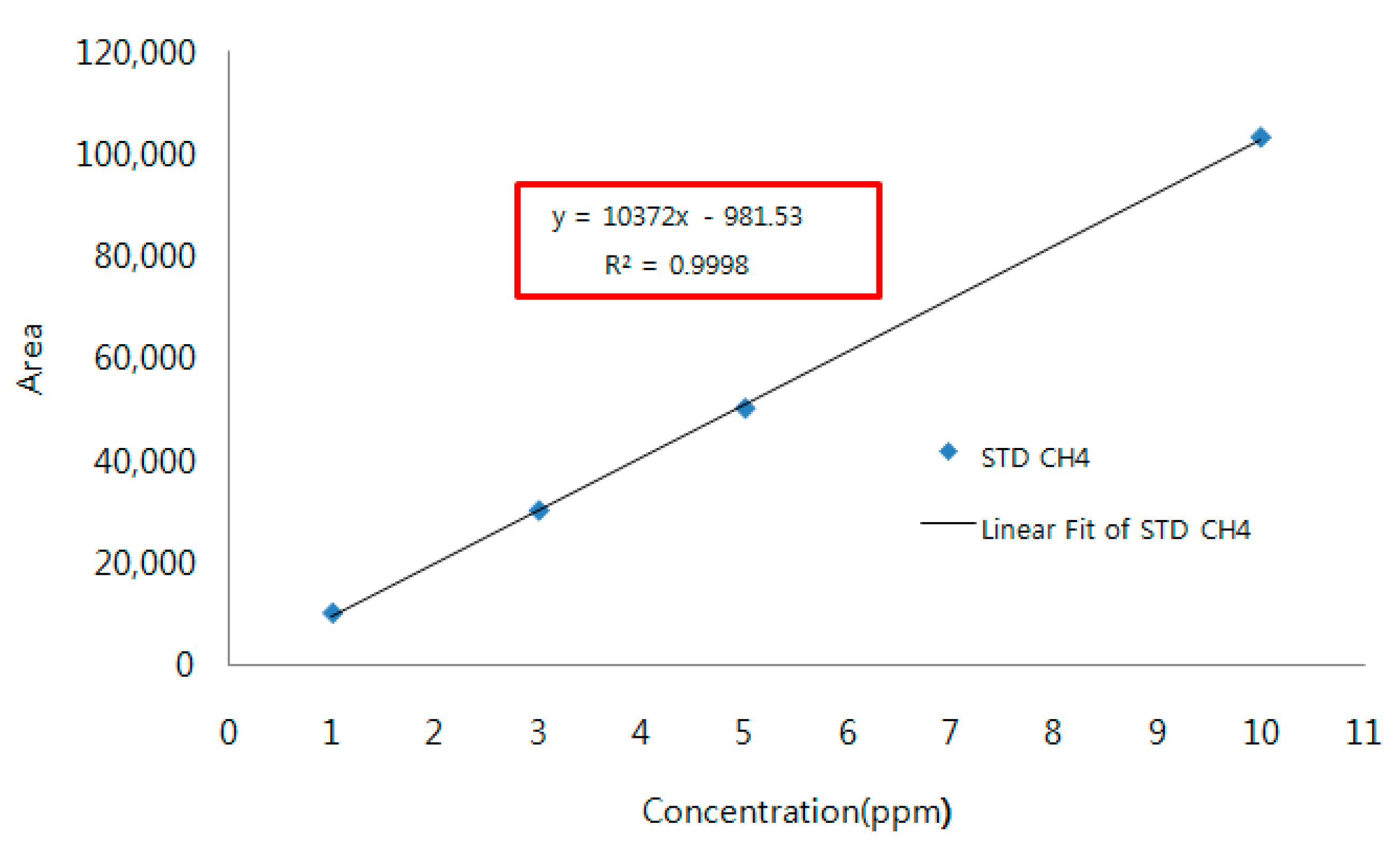
Figure 3.
Process of the Monte Carlo Simulation for estimating the uncertainty of the emission factor.
Figure 3.
Process of the Monte Carlo Simulation for estimating the uncertainty of the emission factor.

Figure 4.
The result of the Monte Carlo Simulation for estimating uncertainty of emission factor. (a) Bituminous coal—Tangential firing; (b) Bituminous coal—Opposed-wall firing; (c) B-C Oil—Tangential firing; (d) B-C Oil—Opposed-wall firing; (e) B-C Oil—Internal Engine; (f) LNG—Combined Cycle.
Figure 4.
The result of the Monte Carlo Simulation for estimating uncertainty of emission factor. (a) Bituminous coal—Tangential firing; (b) Bituminous coal—Opposed-wall firing; (c) B-C Oil—Tangential firing; (d) B-C Oil—Opposed-wall firing; (e) B-C Oil—Internal Engine; (f) LNG—Combined Cycle.


Table 1.
Subject facilities and sampling period.
| Site | Capacity (MW) | Fuel Consumption (ton) | Fuel Type | Boiler Type |
|---|---|---|---|---|
| Plant A | 4000 | 13,260,016 | Bituminous Coal | Tangential firing |
| Plant B | 4000 | 13,082,285 | Bituminous Coal | Tangential firing |
| Plant C | 3340 | 10,205,312 | Bituminous Coal | Opposed Wall firing |
| Plant D | 1400 | 753,354 | Bunker-C oil | Opposed Wall firing |
| Plant E | 150 | 215,040 | Bunker-C oil | Tangential firing |
| Plant F | 40 | 94,349 | Bunker-C oil | Internal Engine |
| Plant G | 1800 | 1,954,381 | LNG | Combined Cycle |
Table 2.
Condition of gas chromatography-flame ionization detection (GC-FID) for CH4 concentration.
| GC/FID | ||
|---|---|---|
| Column | Porapack Q 80/100 | |
| Carrier Gas | N2 (99.999%) | |
| low | Column | 30 mL/min |
| H2 | 30 mL/min | |
| Air | 300 mL/min | |
| Temperature | Oven | 80 °C |
| Injector | 100 °C | |
| Detector | 250 °C | |
| Detector Range | 0 | |
Table 3.
Method detection limit of CH4.
| Concentration | 1.00 ppm |
|---|---|
| Peak Area | |
| 1 | 11,856 |
| 2 | 11,827 |
| 3 | 11,702 |
| 4 | 11,727 |
| 5 | 11,792 |
| 6 | 11,745 |
| 7 | 11,790 |
| Mean | 11,777 |
| SD | 55 |
| SD × 3.14 | 173 |
| MDL | 10.61 ppb |
Table 4.
The result of exhaust gas analysis and CH4 emission factor.
| CH4 | O2 | Theoretical Air Volume | Air Ratio | Theoretical Exhaust Gas Volume (Dry) | CH4 Emission Factor | ||
|---|---|---|---|---|---|---|---|
| ppm | %(vol) | m3/kg | - | m3/kg | kg CH4/TJ | ||
| Plant A | |||||||
| Fuel type | Bituminous Coal | ||||||
| Boiler type | Tangential firing | ||||||
| Mean | 0.51 | 5.62 | 7.17 | 1.40 | 6.98 | 0.14 | |
| SD | 0.18 | 2.05 | 0.15 | 0.31 | 0.15 | 0.05 | |
| RSD(%) | 35.4 | 36.5 | 2.0 | 22.4 | 2.1 | 33.3 | |
| N | 15 | 15 | 15 | 15 | 15 | 15 | |
| Plant B | |||||||
| Fuel type | Bituminous Coal | ||||||
| Boiler type | Tangential firing | ||||||
| Mean | 0.54 | 5.25 | 7.19 | 1.33 | 7.01 | 0.15 | |
| SD | 0.38 | 0.59 | 0.21 | 0.05 | 0.20 | 0.11 | |
| RSD(%) | 71.7 | 11.3 | 2.9 | 3.9 | 2.8 | 73.1 | |
| N | 32 | 32 | 32 | 32 | 32 | 32 | |
| Plant C | |||||||
| Fuel type | Bituminous Coal | ||||||
| Boiler type | Opposed Wall Firing | ||||||
| Mean | 0.30 | 3.89 | 7.50 | 1.23 | 7.30 | 0.08 | |
| SD | 0.07 | 0.18 | 0.14 | 0.01 | 0.13 | 0.02 | |
| RSD(%) | 22.1 | 4.6 | 1.9 | 1.0 | 1.8 | 20.7 | |
| N | 15 | 15 | 15 | 15 | 15 | 15 | |
| Plant D | |||||||
| Fuel type | B-C oil | ||||||
| Boiler type | Opposed Wall Firing | ||||||
| Mean | 0.69 | 5.89 | 10.60 | 1.39 | 10.01 | 0.17 | |
| SD | 0.37 | 0.01 | 0.01 | 0.01 | 0.01 | 0.09 | |
| RSD(%) | 54.0 | 0.1 | 0.1 | 1.0 | 1.1 | 54.0 | |
| N | 15 | 15 | 15 | 15 | 15 | 15 | |
| Plant E | |||||||
| Fuel type | B-C oil | ||||||
| Boiler type | Tangential firing | ||||||
| Mean | 0.48 | 5.81 | 10.94 | 1.38 | 10.28 | 0.12 | |
| SD | 0.13 | 0.18 | 0.12 | 0.02 | 0.11 | 0.03 | |
| RSD(%) | 27.9 | 3.2 | 1.1 | 1.2 | 1.1 | 26.5 | |
| N | 17 | 17 | 17 | 17 | 17 | 17 | |
| Plant F | |||||||
| Fuel type | B-C oil | ||||||
| Boiler type | Internal Engine | ||||||
| Mean | 1.03 | 14.38 | 10.98 | 3.18 | 10.32 | 0.61 | |
| SD | 0.26 | 0.16 | 0.11 | 0.08 | 0.10 | 0.16 | |
| RSD(%) | 25.4 | 1.1 | 1.0 | 2.5 | 1.0 | 26.5 | |
| N | 27 | 27 | 27 | 27 | 27 | 27 | |
| Plant G | |||||||
| Fuel type | LNG | ||||||
| Boiler type | Combined Cycle | ||||||
| Mean | 0.11 | 13.70 | 10.09 | 2.88 | 8.20 | 0.05 | |
| SD | 0.08 | 0.07 | 0.00 | 0.03 | 0.01 | 0.04 | |
| RSD(%) | 76.93 | 0.5 | 0.0 | 1.0 | 0.1 | 76.93 | |
| N | 41 | 20 | 20 | 20 | 20 | 41 | |
Table 5.
CH4 emission factor and uncertainty rage for each fuel and boiler type of thermal power plants.
Table 5.
CH4 emission factor and uncertainty rage for each fuel and boiler type of thermal power plants.
| Fuel Type | Boiler Type | Emission Factor (kg CH4/TJ) | Uncertainty Rage (%, 95% Confidence) | ||
|---|---|---|---|---|---|
| This Study | 2006 IPCC G/L | This Study | 2006 IPCC G/L | ||
| Bituminous coal | Tangential firing | 0.14 | 0.7 | −46.6~+145.2 | 50~150 |
| opposed wall firing | 0.08 | 0.7 | −25.3~+70.9 | ||
| B-C | opposed wall firing | 0.17 | 0.8 | −47.7~+201.1 | |
| Tangential firing | 0.12 | 0.8 | −39.0~+93.5 | ||
| Internal Engine | 0.61 | - | −38.7~+106.1 | ||
| LNG | Combined Cycle | 0.05 | 1.0 | −89.9~+325.9 | |
© 2018 by the authors. Licensee MDPI, Basel, Switzerland. This article is an open access article distributed under the terms and conditions of the Creative Commons Attribution (CC BY) license (http://creativecommons.org/licenses/by/4.0/).
Share and Cite
MDPI and ACS Style
Cho, C.; Kang, S.; Kim, M.; Hong, Y.; Jeon, E.-c. Uncertainty Analysis for the CH4 Emission Factor of Thermal Power Plant by Monte Carlo Simulation. Sustainability 2018, 10, 3448. https://doi.org/10.3390/su10103448
AMA Style
Cho C, Kang S, Kim M, Hong Y, Jeon E-c. Uncertainty Analysis for the CH4 Emission Factor of Thermal Power Plant by Monte Carlo Simulation. Sustainability. 2018; 10(10):3448. https://doi.org/10.3390/su10103448
Chicago/Turabian StyleCho, Changsang, Seongmin Kang, Minwook Kim, Yoonjung Hong, and Eui-chan Jeon. 2018. "Uncertainty Analysis for the CH4 Emission Factor of Thermal Power Plant by Monte Carlo Simulation" Sustainability 10, no. 10: 3448. https://doi.org/10.3390/su10103448
Note that from the first issue of 2016, this journal uses article numbers instead of page numbers. See further details here.