The Synergy between Aquaculture and Hydroponics Technologies: The Case of Lettuce and Tilapia

Abstract

This study investigates the economic and environmental value of the use of technologies that convert pollution and waste in one production process to an input in another production process. The study focuses on an aquaponics case study to show that the negative externalities borne from intensive fish farming can be internalized without regulatory intervention through a combination of fish farming and hydroponics. The introduction of aquaponics diversified the farmers’ sources of income, yielded savings in the cost of water purification and the cost of fertilizer for the plants’ growth, and resulted in more fish and plant output compared to the unregulated scenario. While deriving these results, we also derive a separation rule for managing live aquatic inventory, which separates expenses (which are affected by the biology of fish) and income.

1. Introduction

Growing environmental concerns caused by the unintended effects of modern agriculture and food systems—through greenhouse gas emissions and air pollution, deforestation, loss of biodiversity and the depletion of wild fisheries—led to the development of policies and technologies aimed at achieving sustainable development. The strategies leading to sustainable development included conservation, renewable energy, and the move from harvesting (hunting) systems to renewable systems of animal husbandry. Key to these strategies is the development of the bio-economy; that is, the development of economic activities that utilize biological resources to produce sustainable production systems of food, chemicals, and energy [1].

While the transition from hunting to farming occurred thousands of years ago, fish mostly remained an outcome of harvesting and wild catch, thus leading to the depletion of wild fish habitats and concerns regarding the sustainability of wild fish populations. Economic forces and technological improvement led to the emergence of fish farming, also known as aquaculture, which refers to the farming of aquatic animals under controlled conditions [2]. These production systems have exhibited one of the world’s highest growth rates among agricultural products in recent decades, with aquaculture’s share of the global output of fish and fish products growing at an average annual rate of 8.8% from 1980 through 2010 [3,4]. In Bangladesh, for example, the farmed fish market has grown by a factor of 25 since the 1990s, reaching almost 2 million metric tons in 2017 [5]. Although not conclusive, the literature offers support for claims that aquaculture reduces poverty and contributes to food security [6] and that the increase of farmed fish increases the consumption of fish among the poor [7]. The phenomenal expansion of commercial aquaculture in Bangladesh is associated with alleviating fish price increases, resulting in the increase of fish consumption by the extremely and moderately poor and by rural populations [8].

The aquaculture system generates a constant supply of fish at an efficient feed-to-output ratio when compared to other livestock technologies. However, aquaculture generates wastewater that contains residuals of uneaten food and high concentrations of nitrogen and phosphorus, which harm the environment and can cause eutrophication [9,10,11]. Recent technological developments led to processes that reuse waste products, in part because of public concerns regarding animal production and waste management [12]. These developments represent a step towards the building of a circular economy, which refers to the development and deployment of technologies that connect processes and businesses through the recycling and reuse of waste and by-products [13]. These processes are widely promoted in Asia and build on the seminal work of [14], which indicates that all material flows need to be accounted for and that their management should be determined by their economic value.

This paper develops a conceptual framework with a numerical application, analyzing the economics of an aquaculture system whose efficacy is enhanced through linkages to hydroponics (i.e., the growing of plants without soil). Under this combined system, the pollution generated by the fish is used as an input in the growing of the plants; thus, “one’s waste is the other’s input.” This system is similar to the fish-rice systems of Bangladesh [15]. We develop a biological-economic model that combines aquaculture with hydroponics. The plants have a role in the water purification process because they absorb the nitrogen and phosphorus that is excreted into the water by the fish, resulting in a reduction in the use of fertilizer in the hydroponics system, which results in a reduction of the production costs. This modeling of the circular economy leads to an important outcome: in the closed combined system, where linkages among hydroponics and aquaculture are created, more output is generated in equilibrium than in the equilibrium of the non-regulated, yet separate, production systems.

Although this paper focuses on intensive large-scale aquaponic systems, the paper’s key findings pertain to any aquaponic system; the magnitude of the effects, however, depends on the synergistic linkages among the various units. Aquaponics refers to systems that combine farming of aquatic organisms with water-based terrestrial plant cultures [16]. Palm et al. [16] revised the COST Action FA 1305 “EU Aquaponics Hub” and redefined aquaponics as follows:

Aquaponics is a production system of aquatic organisms and plants where the majority (>50%) of nutrients sustaining the optimal plant growth derives from waste originating from feeding the aquatic organisms.

Building on their definition, [16] define four aquaponic systems: Rice-Fish Culture (e.g., [17,18,19]), Livestock-Fish Culture systems (e.g., [20,21]), Aquaponics ([22,23]), and Integrated Multitrophic Aquaculture [24]. While in Rice-Fish Culture systems the rice fields receive nutrient-enriched water [16], Livestock-Fish Culture systems use the excrements of goats and chickens as fertilizers to increase algal and fish growth [20,21]. Aquaponic systems use the effluent water for soilless plant cultivation [16], and the Integrated Multitrophic Aquaculture systems’ overarching objective is to feed the more primitive species of organisms with feed remnants of higher-level aquaculture species, thus reducing waste discharged into the environment. Common to all these systems is the use of the fish (and/or higher-level aquaculture species) feed remnants to feed other species of organisms. The underlining structure captured through this paper’s modeling of the circular economy encompasses all these alternative systems, albeit the magnitude of the various effects depends on the specificity of the system investigated—a topic that is outside the scope of this work and that would require the collection of new data pertaining to the specific parameters of the system of interest.

The circular economy introduces sustainable technological advancements to aquaculture. However, the use of waste-to-input technologies requires a diverse set of tools and expertise, which necessitates the development and training of human capital. The implementation of these technologies requires the understanding of two distinct biological systems: fish-based and plant-based systems. We hypothesize that the need for human capital is a key barrier to the adoption of the technologies, because the social benefits of learning and education are not included in the farmers’ calculations. Thus, we conclude that there is a need for market intervention and that institutional change (e.g., extension services) can alleviate the barriers to the adoption of waste-to-input technologies. To this end, policies and incentives that correct market failure yield sustainable development through the strengthening of conservation, recycling, and reuse, as well as the development of the bioeconomy, which builds on biological processes and feedstock to produce renewable biological-based products [25,26].

In Section 2 below, we present the aquaponic systems and model the biological and economic factors; that is, we model the managing of live fish inventory while focusing on aquaculture and hydroponics technologies. This model is calibrated in Section 3, where the results of the numerical model are presented. A discussion and concluding remarks are offered in Section 4.

2. The Case of Aquaponic Systems

The economic activity of fish farming involves biological and economic aspects such as fish growth, quality (e.g., length), market demand, and costs. We present these building blocks below, one at a time, starting with biological growth.

The transition of the approach to fish consumption from maritime hunter-gatherer to husbandry was driven by population and economic growth, factors which led to the depletion of coastal nutrition-rich zones and the stressing of ocean populations (During prehistoric times, the coast of Peru was a heavily populated and thriving region that benefited from gross primary productivity of coastal zones of about 2000 kcal./m²/yr [27]. Such productivity is the outcome of the mixing of cold waters rich in nutrient sediments from ocean depths with warmer sunlit waters from the photosynthetic zone of the ocean surface [28], resulting in technological innovation and in the introduction of extensive aquaculture systems. With extensive fish farming, nature consumes the uneaten food and the high concentrations of nitrogen and phosphorus emitted during farming. These extensive aquaculture systems date back to the Han dynasty (206 AC to 225 BC; [29]), where rice and fish were grown together. The fish-rice systems have a long history in Asia [15]. This technology has been employed in China for two thousand years, with almost 1 million ha in China and 94,000 ha in Indonesia [30]. Culturing fish and Azolla in rice fields is a significant component of organic farming in China [31].

Processes similar to those that led to the transition to husbandry and the introduction of extensive agriculture systems also resulted in the intensification of fish farming practices. The transformation in technology and science, driven by major improvements in the field of biology (groundbreaking research in molecular biology, discoveries in the field of genetics, and improvements in information technologies) yielded ground-breaking changes that resulted in the intensification of agricultural production processes.

The intensification of production of fish farming, also known as aquaculture, exhibited one of the world’s highest growth rates among agricultural products in recent decades [4,5] and is the focus of the analysis below.

2.1. The Biological Growth Process

The age at which fish can be marketed determines the overall biomass of the school of fish and the size of the fish, as well as the amount of food the fish consume and, thus, the pollution generated by intensive fish farming. Building on the growing inventory models of [32,33] and others, we developed a biological model that accounts for the biomass of fish, the amount of feed, and the size of the fish. Specifically, we assume the following:

• The weight of the school of fish, denoted as B_a, is described by a function that depends on the age of the fish measured in weeks, denoted as t; that is, $B_a=b_a\left(t\right)$, where ${b_a}^{\prime }\left(t\right)>0$ and ${b_a}^{″}\left(t\right)<0$ [34]. Although in the numerical analysis we assume fish fatalities, in the conceptual analysis below we abstract from this parameter.
• Food consumption is a function of the weight of the fish [35]. Technically, we assume that the weight of the fish is a function of their age and ad-libitum feeding, resulting in fish feed that is a function of the age of the fish; that is, $X_a=x_a(t)$, where ${x_a}^{\prime }\left(t\right)>0$ and ${x_a}^{″}\left(t\right)<0$.

Fish need energy to maintain life and grow. Although the growth rate of fish slows as they get older, they require more energy as they get older because of the need to sustain their size [35,36] (Although feeding affects both growth and maintenance [34,35] the relation between biomass and feed remains one-to-one; for brevity and simplicity, we abstract from maintenance in what follows.). Because we assume a one-to-one relationship between weight and feed, and the age of the fish and feed, the biomass of the school of fish can be expressed as a one-to-one relationship between the weight of the fish and the fish feed; that is, $B_a=b_a(x_a^{-1}(t))$.

In recent years, consumers’ preferences for quality of fish increased. European, Japanese, and U.S. consumers are looking for diversity, freshness, and convenience. Many consumers prefer fresh products, and the share of fresh fish in international trade has increased in recent years [37]. Although quality, denoted as Q_a, can be expressed in several ways, we based the quality of the fish on their length, which is a function of their age. “Plate size” fish cost more than either smaller fish or larger fish, where the index, $\tilde{t}$, indicates the age at which fish reach plate size. Assume $Q_a=q_a\left(t\right)$, where

$$q_a^{\prime }\left(t\right)=\{\begin{array}{cc}>0& fort<\tilde{t}\\ =0& fort=\tilde{t}\\ <0& Otherwise\end{array}$$

Similar to the fish weight, we assume that the length of fish from head to tail, $Q_a=q_a\left(x_a^{-1}\left(t\right)\right)$, can be expressed as a one-to-one relationship between the length of fish and its feed. The aforementioned assumptions, then, imply that we can define an index $Y_a=y_a(B_a,Q_a)=y_a(x_a^{-1}(t))$, where ${y_a}^{\prime }\left(t\right)>0$ and ${y_a}^{″}\left(t\right)<0$.

Our assumptions yield an autonomous problem: time does not appear explicitly in the biological model; rather, it affects fish growth implicitly via the fish’s growth function. The manager of the intensive fish farming system decides on the optimal age at which to harvest the fish independent of the investment decision. Because our problem does not explicitly include time, it is reasonable to expect that the solution to our maximization problem is a stationary solution [38].

The intensive aquaculture system is a reliable technology that generates a constant supply of fish at an efficient feed-to-output ratio when compared to other livestock technologies. However, aquaculture generates wastewater that contains residuals of uneaten food and high concentrations of nitrogen and phosphorus that harm the environment and can cause eutrophication [9,10,11]. Although aquaculture can provide ecosystem services, such as wastewater treatment, bioremediation, and habitat structure, it also can be used inappropriately with serious negative ramifications to the environment. Its use can degrade the quality of freshwater and that of the ecosystem at large, resulting in health risks ([9], and references therein).

2.2. Aquaculture and the Environment

Before discussing aquaculture and the implications of environmental policy, prices are introduced. The price of a single fish is determined by two variables: the weight of the fish and its length. That is, revenues $R_a=p_a\times {\mathrm{Y}}_a$, where $p_a$ is the price per unit of biomass; note that our assumptions suggest $R_a^{\prime }>0$ and $R_a^{″}<0$. In addition, let $w_a$ denote the price of input, $X_a$.

Next, note that fish breeding systems accumulate nitrogen and phosphorus that are excreted into the environment as pollutants that must be discharged (i.e., $z_a$). The environment has low absorptive capacity, and the pollutant accumulates overtime. In the absence of an appropriate policy, fish growers will not account for this cost, despite the fact that the failure to do so generates a negative social cost. One way of dealing with this failure is a Pigovian tax. This approach will cause growers to reduce the amount of pollution they produce [9,39], resulting in higher fish prices. For simplicity, assume that fish growers pay taxes when harvesting and marketing the fish. Let $z_a$ denote the monetary damage associated with the accumulated nitrogen and phosphorus that have been emitted. Because of the relationship between the feed, weight, and length of the fish, $Z_a$=${\displaystyle \sum }_{j=0}^t{z}_a\left(x_a(j)\right)$ increases in the amount of feed at an increasing rate; that is, $z_a^{\prime }(\cdot )>0$ and $z_a^{″}(\cdot )<0$.

When regulation levies a tax on pollution, the profit function of the fish grower is defined by Equation (1), in which k₀ denotes the interval of time investigated (e.g., ${\mathrm{k}}_0=52$ weeks). In the absence of a technology that can convert waste into an input, the aquaculture unit maximizes the following profit function:

$${\mathsf{\pi }}_a=\left(p_a\cdot Y_a-w_a\cdot X_a-\tau \cdot Z_a-\mathrm{t}\cdot F{C}_a\right)\cdot \frac{{\mathrm{k}}_0}{\mathrm{t}}$$

(1)

Let ${\mathrm{C}}_a\equiv w_a\cdot X_a$ and ${\mathsf{\Psi }}_a\equiv \tau \cdot Z_a$, where $\tau$ denotes the pollution tax. Equation (1) suggests that expenditures for the treatment of contaminants essentially are similar to expenses incurred to feed the fish. The basis for this comparison is the one-to-one relationship between the feed and the age of fish, as well as the weight and the feed, and pollution. Also, let $F{C}_a$ denote the weekly costs that do not depend on the age of the fish.

Fish feed, which includes fish meal, is key to the sustainability of aquaculture technologies, especially when feeding carnivorous or omnivorous species. Fish meal is the product of harvesting small, oily fish that belong to low trophic levels. Both the fisheries of fish feed (i.e., reduction fisheries) and wild populations are overexploited [39,40], as a result, the success of aquaculture is dependent on progress made in the rationalization of fish meal inputs [41,42]. To this end, research has inquired into the sustainability of fish meal using plant or terrestrial animal-based feed [43,44]. Soy meal has emerged as a good substitute. However [41] work suggests that beyond a certain degree of replacement, farmed fish species suffer from a decline in growth under a soy-based diet. Microalgae is also a candidate to substitute for fish meal; however, cost prohibits its wide deployment [45,46]. A plant-based meal that is much simpler to harvest than microalgae and is a complete (whole) protein (not a partial protein like, e.g., soybeans) is duckweed. Work done by [47], as well as ongoing work of the present author, suggests that duckweed can replace 50% of fish meal with no statistical impact on growth. As that research shows, the benefits are not only in reducing demand for fish meal but also in cutting feeding costs by about 40%. Because this topic, although important, is outside the scope of this work, hereinafter we assume a generic feed source $X_a$ that costs $w_a$ per unit of feed.

Within the length of the period investigated, k₀, the weekly expenses and the investment in the farm (e.g., buildings, containers) were not included in deciding the optimal age for marketing the fish. However, expenses and investment will be needed to determine the conditions of entry to the industry. Time does not explicitly affect the farmer’s harvesting decisions, but it does affect his investment decisions. Note that we are ignoring the effect of the interest rate, which is assumed to be negligible given the units of time that are being considered.

Next, we investigate the first-order conditions and derive a simple harvesting decision rule. The first-order condition of Equation (1) is:

$$\frac{{\mathrm{d}\mathsf{\pi }}_a}{\mathrm{dt}}\equiv \underset{\begin{array}{c}\% change in \\ revenue\end{array}}{\underbrace{\frac{\mathrm{d}{R}_a}{\mathrm{dt}}\frac{1}{R_a}}}{R}_a-\underset{\begin{array}{c}\% change in \\ feed cost\end{array}}{\underbrace{\frac{{\mathrm{dC}}_a}{\mathrm{dt}}\frac{1}{{\mathrm{C}}_a}}}{\mathrm{C}}_a-\underset{\begin{array}{c}\% change in \\ cost \\ of pollution\end{array}}{\underbrace{\frac{{\mathrm{d}\mathsf{\Psi }}_a}{\mathrm{dt}}\frac{1}{{\mathsf{\Psi }}_a}}}{\mathsf{\Psi }}_a=\underset{\begin{array}{c}Average profit \\ per unit of time\end{array}}{\underbrace{\frac{R_a-{\mathrm{C}}_a-Z_a}{{\mathrm{t}}^{\ast }}}}\equiv \frac{{\mathsf{\pi }}_a}{{\mathrm{t}}^{\ast }},$$

(2)

where ${\mathrm{t}}^{\ast }$ denotes the optimal marketing age of the fish. Equation (2) indicates that the optimal time to harvest of a batch of fish is when the marginal benefit of marketing the fish is equal to the average cost of keeping the fish batch for one more week (Figure 1, point R). Equation (2) is a simple decision rule, which is the outcome of the separation between the cash flow that depends on the growth curve of the fish and the cash flow that does not. Because of the separation between income and expense, which depend on prices and quantities and on the biological growth curve, respectively, this decision rule requires only a limited amount of data.

Because of the drastic decline of the world’s fishery resources, aquaculture is being promoted to supply fish and shellfish to meet society’s increasing demands. The expansion of aquaculture has been given high priority on a global basis [4,48]. However, introducing pollution into the aquaculture manager’s decision process shifts the marginal and average profit curves down and to the left, producing curves that intersect at point R in Figure 1, clearly indicating that regulation had a negative effect on the profitability of fish farming.

Recent technological developments led to processes that harness waste and pollution and convert them into inputs. Some of these developments were in response to increasing public concerns regarding livestock production and waste management [12,49]. The advancements in the development and deployment of these technologies is generalized through the concept of the circular economy [13,14]. More specifically, the choice of the fish-farming technology may eliminate pollution while yielding lower fish prices. We will show below that the building of an aquaponics supply system can eliminate the pollution caused through aquaculture at a lower fish price than under the regulatory outcome.

2.3. The (Circular) Aquaponic Systems

The aquaponic systems maintains a balance between the number of fish and the quantity of plants. The inputs of this system include fish food, seeds, water, electricity, and the small amounts of calcium (Ca), potassium (K), and iron (Fe) required for the plants [50]. Then, given the biological and economic parameters, we can obtain the plant biomass required to remove the pollution that the fish introduce into the water.

Assume that technological advancements led to the introduction of a production process $\mathsf{\Theta }=f_{\Theta }\left(z_a\right)$, where $f_{\Theta }^{\prime }(\cdot )>0$ and $f_{\Theta }^{″}(\cdot )<0$, that uses pollution and waste, $z_a$, to generate an input $\mathsf{\Theta }$, where we assume that the market price of $\mathsf{\Theta }$ is $w_{\Theta }$. This technology converts toxic pollution, $z_a$, into an input $\mathsf{\Theta }$ at a cost of $C_{\Theta }\left(z_a\right)=C_{\Theta }\left(w_{\Theta },\Theta \right)$, and there is a fixed cost of $F{C}_{\Theta }$. In addition, let the rent from owning this technology be

$${\pi }_{\Theta }=w_{\Theta }\cdot \mathsf{\Theta }-C_{\Theta }\left(w_{\Theta },\Theta \right)-F{C}_{\Theta }.$$

(3)

The hydroponics production process uses input $X_h$ (for simplicity, we assume $\mathsf{\Theta }$ is equivalent to $X_h$) to produce output $Y_h=y_h\left(X_h\right)$. Let $w_h$ denote the price of input, $X_h$, and let $p_h$ denote the price of output, $Y_h$, such that revenues are ${\mathrm{R}}_h(\cdot )$. Let the rent from owning the hydroponics technology be

$${\pi }_h=p_h\cdot Y_h-w_h\left(X_h-\Theta \right)-w_{\Theta }\cdot \mathsf{\Theta }-F{C}_h,$$

(4)

where $F{C}_h$ denote the fixed costs.

How does the introduction of an aquaponic systems—a system that combines aquaculture with hydroponics in a symbiotic environment—affect the equilibrium outcome? To answer this question, we modify Equation (1) as follows:

$${\mathsf{\pi }}_a^{\ast }=\left(p_a\cdot Y_a-w_a\cdot X_a-\tau \cdot \left(Z_a-\Theta \right)-\mathrm{t}\cdot F{C}_a\right)\cdot \frac{{\mathrm{k}}_0}{\mathrm{t}}$$

(5)

In other words, the pollution generated through aquaculture production is redirected to the waste-to-input technology, where the cost of collecting and redirecting the pollution $Z_a$ to the production of $\mathsf{\Theta }$ is embedded in $C_{\Theta }\left(w_{\mathsf{\Theta }},\mathsf{\Theta }\right)$. This solution incorporates the benefits from the introduction of the circular system, specifically the use of the waste from one process as the input to another process. Then, if $w_{\Theta }\le w_h$, aquaponics will lower the cost of the fertilizer. Because older fish produce more pollution, the saving in fertilizer costs increases as the age of the fish increases. In an internal solution, the objective function of the aquaponic systems, $\mathsf{\Pi }\equiv {\mathsf{\pi }}_a^{\ast }+{\mathsf{\pi }}_h+{\mathsf{\pi }}_{\mathsf{\Theta }}$, is:

$$\mathsf{\Pi }=\left[\left({\mathrm{R}}_a-{\mathrm{C}}_a-\mathrm{t}\cdot F{C}_a\right)+\left({\mathrm{R}}_h-C_{\Theta }\left(w_{\Theta },\Theta \right)-\mathrm{t}\cdot \left(F{C}_h-F{C}_{\mathsf{\Theta }}\right)\right)\right]\cdot \frac{{\mathrm{k}}_0}{\mathrm{t}}$$

(6)

Thus, we get the following rule for deciding the optimal harvest time, where

$${\mathrm{t}}^{\mathrm{as}}=argma{x}_t\mathsf{\Pi }$$

${\mathrm{t}}^{\mathrm{as}}$ denotes the optimal length of the harvesting cycle when using an aquaponic systems:

$$\frac{\mathrm{d}\mathsf{\Pi }}{\mathrm{dt}}=\underset{\begin{array}{c}\% change in \\ revenue\end{array}}{\underbrace{\frac{\mathrm{d}\left({\mathrm{R}}_a+{\mathrm{R}}_h\right)}{\mathrm{dt}}\frac{1}{\left({\mathrm{R}}_a+{\mathrm{R}}_h\right)}}}\left({\mathrm{R}}_a+{\mathrm{R}}_h\right)-\underset{\begin{array}{c}\% change in \\ feed cost\end{array}}{\underbrace{\frac{\mathrm{d}\left({\mathrm{C}}_a+C_{\mathsf{\Theta }}(\cdot )\right)}{\mathrm{dt}}\frac{1}{\left({\mathrm{C}}_a+C_{\Theta }\right)}}}\left({\mathrm{C}}_a+C_{\Theta }(\cdot )\right)=\frac{\left[\left({\mathrm{R}}_a+{\mathrm{R}}_h\right)-\left({\mathrm{C}}_a+C_{\mathsf{\Theta }}(\cdot )\right)\right]}{\tilde{\mathrm{t}}}=\frac{\mathsf{\Pi }}{\mathrm{t}}$$

(7)

To compare the aquaponic systems outcome with the two other outcomes (i.e., the regulated and the unregulated one), define the following:

$${\mathrm{t}}^{\mathrm{r}}=argma{x}_t{\mathsf{\pi }}_a^{\mathrm{r}}$$

$${\mathrm{t}}^{\mathrm{nr}}=argma{x}_t{\mathsf{\pi }}_a^{\mathrm{nr}}$$

Then, the equilibrium outcome is such that ${\mathrm{t}}^{\mathrm{as}}\ge {\mathrm{t}}^{\mathrm{nr}}\ge {\mathrm{t}}^{\mathrm{r}}$. Internalization allowed the aquaponics technology to replace the environmental policy, and this resulted in marketing the fish at an older age. Technically, the average profit and the marginal profit shift upwards and to the right, and they intersect at point A in Figure 1. The new equilibrium intersection is above and to the right of point R, indicating that aquaponics both eliminated the pollution and reduced the cost of the fertilizer needed for the plants (recall that we assumed $w_{\Theta }\le w_h$).

When hydroponics technologies are introduced, and assuming that hydroponics technologies are used in conjunction with aquaculture technologies, an equilibrium outcome is achieved that dominates the regulated solution, both economically and environmentally (Figure 1, point A versus point R). The long-term economic success of aquaculture systems depends on the ecosystem’s capacity to support technologies that provide fish and shellfish for human consumption. Trying to eliminate resource fluctuations and make society independent of nature may be successful in the long run only if this effort accounts for the ecological, economic, and social costs incurred by intensive fish farming [51,52]. Aquaponics technology can achieve this goal and offer a sustainable solution.

3. The Numerical Model

3.1. The Calibration of the Numerical Model

We use a numerical example to get a better understanding of the outcome of our model. The numerical model focuses on systems that are based on aquaculture. When modeling the hydroponic system, we focused on the steady state and assumed staggered harvesting (i.e., the plants are harvested every week at a constant rate).

The first step of the numerical analysis was to calibrate the numerical model, where we introduced explicit functions for quality of fish and pollution-generation.

3.1.1. The Quality Function

For the quality function, we used a distribution function that is similar to the gamma function, with a maximum of 1 and a minimum of 0:

$${\mathrm{q}}_a\left(\mathrm{t}\right)=\frac{\mathrm{t}\times {\mathrm{e}}^{1-\mathrm{t}/\mathsf{\psi }}}{\mathsf{\psi }}$$

(8)

where $\mathsf{\psi }$ is a parameter; in the following, we assume that $\raisebox{1ex}{$\mathrm{t}$}\!\left/ \!\raisebox{-1ex}{$2$}\right.<\mathsf{\psi }$. The maximum of ${\mathrm{q}}_a(\cdot )$ is obtained when the fish reach the age of $\mathsf{\psi }$, which is the age at which the length of the fish is of the best quality (i.e., plate size).

3.1.2. The Pollution Generating Functions

To calculate the amount of nitrogen and phosphorus excreted by the fish, we must calculate the amounts of nitrogen and phosphorus that enter the system and their uses. The remainder (i.e., the amount of each that is not used) is the amount excreted into the water [53].

To calculate the net mass balance of nitrogen and phosphorus, we add the amounts that the plants absorb and the amounts that accumulate in the tissues of the fish, and we subtract the amounts of nitrogen and phosphorus excreted into the water by the fish. The amounts excreted are multiplied by the purification cost of nitrogen and phosphorus. We use these measures to calibrate the system so that the amount of plants matches the amount required to remove all of the nitrogen and phosphorus from the water (Appendix A). In very intensive aquaculture production systems that use pure oxygen, carbon dioxide is a limiting water quality parameter—especially when the dissolved oxygen concentration is controlled [54]. The accumulation of carbon dioxide can lead to reduction in the pH, resulting in reduction of the mole fraction and concentration of un-ionized ammonia [55]. A mole of carbon dioxide is produced for every mole of oxygen consumed by fish; that is, on a mass basis, 1.38 g of carbon dioxide is produced for every 1 g of oxygen consumed by fish. Carbon dioxide is produced by the fish at a greater rate than oxygen is consumed. In this work, we assume that a CO₂ stripping tower is used to strip the CO₂ from the water, and this impacts the capital cost of the aquaculture system.

3.2. The Outcome of the Numerical Model

We assume a model of an aquaponic systems that grows tilapia and lettuce. The type of fish we selected was tilapia because of its tolerance of intensive fish-farming systems. Lettuce was chosen because it can absorb large amounts of nitrogen from the water [50,56].

We assumed an annual output of 40 metric tons of tilapia. To achieve this goal, we aimed for a weekly output from the system of 770 kg. The number of fish in each group of fish and biomass data were obtained from [57]. The data for the weight per fish for a period from 0 to 40 weeks were 0.5 g and 750 g, respectively. The data included the length and weight of the fish, the amount of food provided daily, and the feed conversion ratio. We also assumed that the lettuce would be harvested each week and that a constant number of lettuce heads was harvested. Since the analysis was done for a period of 52 weeks (${\mathrm{k}}_0=52$), we used these data from the 40-week period to predict the amount of feed and the biomass of the fish for the entire 52 weeks.

We calibrated the quality curve such that the maximum price per kg of tilapia was achieved at $\mathsf{\psi }=18$. The other biological and economic parameters are presented in

Table 1. Biological and economic parameters.

Parameter	Value	Source	Description
P1	10.9 NIS	[58]	Price per kg of tilapia
g1	2.5 NIS	[58]	Price per kg of fish food
NitV	0.34%	[59]	Percentage of nitrogen in lettuce
PhoV	0.075%	[59]	Percentage of phosphorus in lettuce
NF	5.6%	[60]	Percentage of nitrogen in fish food
PP	35%	Commercial food supplier	Percentage of protein in fish food
PF	1.1%	Commercial food supplier	Percentage of phosphorus in fish food
DMF	26.5%	[53]	Percentage of dry matter weight of fish
${\mathrm{Nit}}_{\mathrm{F}}$	8.5%	[53]	Percentage of nitrogen in fish
${\mathrm{Pho}}_{\mathrm{F}}$	3.01%	[53]	Percentage of phosphorus in fish
${\mathrm{g}}_{\mathrm{N}}$	14.7 NIS	[59]	Price per kg of nitrogen from water purification
${\mathrm{g}}_{\mathrm{P}}$	47.06 NIS	[59]	Price per kg of phosphorus from water purification

.

When choosing the optimal weight of the fish in the unregulated scenario, we used the simple decision rule. The calibrated model without external costs results in the marginal profit being equal to the average profit in week 37, with the weight of the fish at 600 g. However, when the external costs (i.e., the marginal cost of purifying water) are taken into account by the grower, Equation (2) equalizes the profit margins with the average at 32 weeks, when the fish weigh about 410 g. Thus, when the grower’s external costs are considered, the grower grows the fish for a shorter period of time, because the marginal gain from waiting another week is smaller than the marginal costs (Figure 2). In the regulated scenario, the marketed fish biomass decreases and the price per fish increases. Note that the profitability of the aquaculture system is lower than that of an aquaponic systems, where the marginal profits is equal to the average profits in week 38, with the weight of the fish at 700 g (Figure 3).

The conceptual analysis shows that the optimum age for marketing fish is obtained only on the basis of income and expenses (i.e., food and pollution), and both vary with time. The growth of lettuce is introduced to the expenditure growth cycle, which is constant in the current numerical example (i.e., buying seeds, costs for preparing the surface for fertilizer, costs of harvesting, and the costs of sorting and packaging materials).

Table 2. Profit after direct expenses for fish farming, hydroponic growing, and aquaponics.

	Only Aquaculture	Only Hydroponics	Aquaponics	Savings from Combination
Annual throughput (metric tons)	40	547	587
Revenue (NIS)	436,000	2,392,757	2,841,821
Total direct expenses (NIS)	212,699	1,076,316	1,160,047
Total earnings after direct expenses (NIS)	223,301	1,316,441	1,681,774
Total savings from the combination (NIS)				142,032

compares the earnings after direct expenses for the activities associated with farming fish and lettuce using aquaculture, hydroponics, and aquaponic systems. The total cost savings from the aquaponic systems is estimated at approximately 142,000 NIS per year. Aquaponics results in savings with regard to the cost of pollution due to the decrease in the need for nitrogen and phosphorus fertilizer for the plants. Thus, the aquaponics technology resulted in a solution that yields more fish, minimizes adverse environmental impacts, and has a much lower economic cost than a regulatory environment (Figure 1, point A versus point R; see also Figure 3). The resulting cost is instead to commercial fishing (which faces a lower price for the product) and to fertilizer companies (assuming fertilizer sales decrease).

The economic model describes the cost and revenues associated with aquaponics. The outcome of this model is used to determine the viability of the aquaponic system. The various biological and costs parameters assumed in the analysis are depicted in Appendix B, for both the fish and the lettuce. The data was converted to NIS assuming an exchange rate of 3.6 NIS/US$.

Another advantage of the aquaponic systems, which is not accounted for in the current analysis, is the low variance in the amount of nitrogen that is secreted into the water due to the fact that only 9% of the fish is harvested every week. Then, because we assumed a weekly harvest of a constant number of heads of lettuce, the effect of any reduction of the amount of nitrogen secreted is small. Thus, a continuous and regular flow of income and expenses can be maintained, and a fixed-size staff can be maintained as well.

The analysis identified key factors that affect the economic viability of the aquaponics system, and it also highlighted key barriers to the extensive use of the technology. The choice of fish that have a higher price per kilogram, such as mullet or barramundi (both of which have consumer prices double that of tilapia) can lead to a different distribution of income along the intensive fish-farming supply chain. Also, ornamental fish, such as koi or garra rufa fish, could be grown; in this case, the income from fish farming would be increased, because these fish have higher values per kilogram than tilapia. Preliminary work with the garra rufa suggests that the production of 15,000 fish and 400 lettuce units yields an operating profit of 14,664 NIS, where the direct costs are 31,136 NIS and the investment is 79,000 NIS. The fish were grown from 0.5 cm/0.5 g to 3 cm/3 g in 9 weeks. The price of a garra rufa of 3 cm/3 g is 3 NIS per fish (the 3-week-old fingerlings were bought at 1 NIS per fish). Differing from the tilapia-lettuce system, the garra rufa-lettuce system resulted in 80% of the revenues coming from the fish. Alternative plants could also be used in the hydroponic system, such as a combination of herbs that have a higher value than lettuce and thereby reduce dependence on the demand for one product (in this case, lettuce), resulting in an increase in the fish farmer’s income. These examples emphasize the significance of the input and output prices as well as their implications for the applicability of a viable aquaponics system. The way the supply chain of an aquaponics system is developed (including the choice of fish and plants) has important implications for its economic viability.

4. Institutional Innovation and the Adoption of Circular Systems

The aquaponics production process applies the fundamental concept of the circular economy, which here refers to the connecting of fish and plant production processes through the recycling and reuse of the fish excretion [7]. Although we showed the significant advantages of aquaponic systems, in practice the use rates of these technologies are low. We predict that the disadvantage of combining fish farming with hydroponics plant growth is that the increased need for fish will require expertise in both cultivation and fish farming. Without the knowledge required for cultivation, the fish grower must hire an expert to care for the plants. Another barrier to the use of aquaponic systems is the technical difficulty of creating a system that obtains an optimum growth environment for both the fish and the plants. While nitrifying bacteria and plants thrive at certain pH levels, fish survive at different pH levels, and this creates an ecological engineering challenge in the proposed closed system [61] (Aquaponic systems, in the past, connected aquaculture and hydroponic units through a single closed loop, where water flows from the aquaculture unit to the hydroponic unit and back. In response to the concern of managing a system with a single pH level, de-coupled aquaponics units, which enable better regulation of pH levels in the aquaculture and hydroponics units, were introduced. Results of experiments done with these systems suggest higher yield in the de-coupled system [62], see also [16]. To this end, the best availability of nutrients is guaranteed at a pH of ≤6.5 for hydroponics [63], but the optimal level for a RAS is at ≥7.0 because of the need to ensure conditions for microbial nitrification and thus fish welfare [64]). The effect of aquaculture on fish meal and fish oil is yet another challenge [9,47]. All these barriers suggest that human capital in combination with knowledge of both systems is vitally important for the success of aquaponic systems. Efficient management of both intensive fish farming and plant cultivating must be implemented from both behavioral and engineering perspectives.

What causes viable technologies to be adopted? What leads technologies that are environmentally sustainable and economically viable to be commercially adopted and widely diffused among farmers? The introduction of new technologies results in the shifting of demand for human capital up and to the left. However, industrialization led to competition for human capital and thus to migration to urban areas [65], yielding a substantial increase in the relative factor price of the input. The competition for a resource with an inelastic supply curve leads to substantial barriers to the adoption of technologies that depend on human capital, including aquaponics. Therefore, we believe institutional innovation should accommodate the transition to aquaponic systems in order to improve the efficacy and sustainability of food production.

Below, we discuss alternative paths the regulator may use to achieve high rates of adoption of the technology:

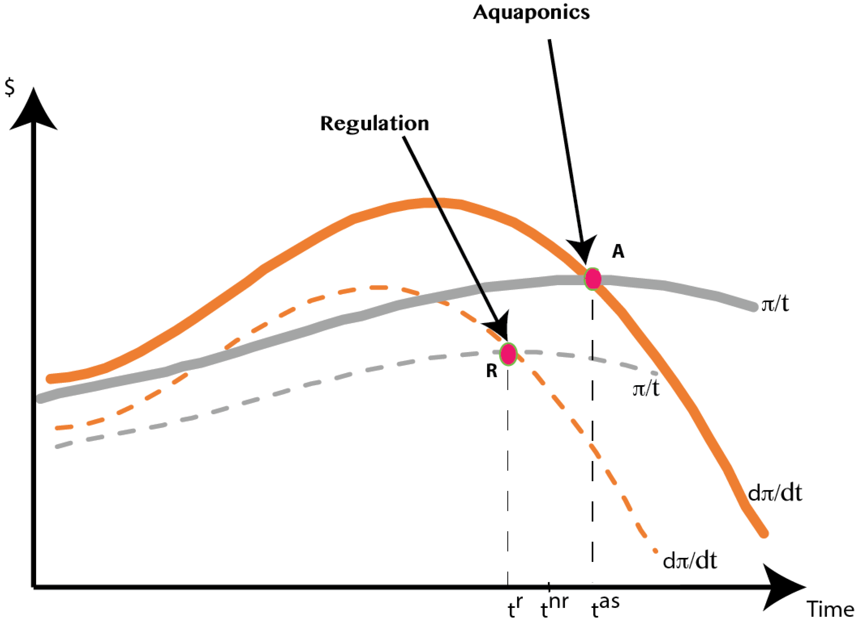
• Pigouvian tax [66]: Section 2.2 showed that if the regulator levies a pollution tax, output declines while prices increase relative to the no-regulation scenario. Regulation results in a sustainable solution that accounts for the social cost of pollution but at higher fish price [67] argued that the need for a core of high-quality individuals is key to the success of regions with challenging conditions. In principle, such a core of high-quality individuals can learn to manage two distinct biological systems; that is, they can learn to grow fish and plants together in closed systems. Under these conditions, a tax will not result in higher prices but will encourage the high-quality individuals to invest in the waste-to-input technology. However, it is likely that extension services are still needed to make the individual farmers aware of the alternative technology and its benefits.
• Institutional change: To promote the adoption of aquaponic systems, the regulator may rely on institutional change. Regional cooperation and/or the development of extension services that facilitate the communications between fish producers and plant growers may result in an increase of adoption rates of aquaponics technologies.
  • Extension services: Extension services, for example, played an important role in the adoption of aquaculture-agriculture systems in Malawi. The extension services made the farmers aware of the technology, and among all adopters, higher benefits are reported for more educated farmers [7]. Technically, the regulator’s choice of institutional change results in extension services that support, educate, and teach, the aquaculture farmers of the management of the circular system. The extension services significantly reduces the cost of learning and thus substantially increases adoption rates of the waste-to-input technology (see also bullet IV.I).
  • Cooperatives: A different solution to extension services was implemented in the Arava, a water-scarce region located at the southern corner of Israel just above the Red Sea and bordering Jordan. Cooperatives were established in the Arava in the 1960s. Two different types of cooperatives were established: the kibbutzim (a community settlement, usually agricultural, organized under collectivist principles) and the moshavim (an entity that is similar to the kibbutzim and emphasizes community labor but supports private ownership of farms of fixed sizes). The cooperative institutions that supported the development of Arava led to the extensive use of drip irrigation, mechanization, and heat treatment to combat pests without the use of chemicals. The cooperatives in the Arava also led to extension services and public investments in R&D [68]. Over time, the Arava became a very profitable agricultural region. It is interesting to note that, with the passage of time, the ownership structure in the moshavim shifted from collectivist principles to private ownership, but the research entity was kept public. The nature of the technology defined the ownership structure over time (i.e., private versus public). To this end, mechanization led to date plantations being mostly managed under collectivist principles, while labor-intensive vegetable and spring crops ended up being managed under private entrepreneurship. When the regulator’s goal is to promote a region populated with many aquaculture and hydroponics farms, the creation of a cooperative leads to a reduction in the cost of learning through the creation of public R&D and extension services borne from the cooperative resources.
  • Outsourcing: Farmers may separate the activities among the three production processes (i.e., aquaculture, waste-to-input, and hydroponics), where the waste-to-input technology is managed by the entrepreneur, who offers services to a region with many aquaculture and hydroponics farmers. Although outside the scope of this paper, the proposed supply chain shifts most of the risk, and therefore most of the economic benefits, to the entrepreneur.

5. Concluding Remarks

To meet the drastic global increase in the demand for fish, intensive fish farming has been widely adopted globally. Most of the aquaculture worldwide uses freshwater, which accounts for 60% of the total tonnage produced by aquaculture [3,4]. This phenomenal expansion of the aquaculture industry has led to the deterioration of water bodies used for human consumption [69] and to the eutrophication and nitrification of ecosystems. For instance, globally the mean feed conversion ratio for shrimp aquaculture is 1.8, indicating that 5.5 million tons of organic matter, 360,000 tons of nitrogen, and 125,000 tons of phosphorous are discharged to the environment every year [70]. Shrimp production represents around 8% of the total aquaculture production. Using these numbers, and following [71], assume similar feed conversion ratios for other farmed organisms, and that the diet formulations has some similitude. Then, feed yields total discharge of wastes that is 12.5 times larger than that calculated under [70]. If not addressed and managed responsibly through policy and/or technology, aquaculture can degrade the ecosystem ([9], and references therein).

This paper showed that the advantage of the circular aquaponic systems is that they internalize the negative externalities of intensive fish farming through their internalization of a positive externality generated by the combination of aquaculture and hydroponic systems. In practice, however, the use rates of aquaponics technologies are low, despite the fact that the expansion of aquaculture, and thus wastewater, is significant. We conclude that efficient management of both intensive fish farming and plant growing must be implemented from both behavioral and engineering perspectives, and we argue that institutional change can foster this transition.

In this work, we did not account for the price of land, and we did not introduce uncertainty. Both of these factors are important to our understanding of aquaponic systems, and we intend to investigate both topics in future work. However, we do not expect such future work to result in qualitative changes in our main results; rather, we expect it to alter the magnitude of the impact of the various effects identified in this study. In our future work, we also plan to compare and evaluate competing technologies, including aquaponic systems and recirculating aquaculture systems (RASs), as well as formally model alternative aquaponic systems (i.e., Rice-Fish-Culture, Livestock-Fish Culture, and Integrated Multitrophic Aquaculture). We suspect that the synergistic linkages among the subsystems will impact yield and profitability and that the magnitude of these effects will be the outcome of the calibrated parameters.

References

1. Zilberman, D. The economics of sustainable development. Am. J. Agric. Econ. 2013, 96, 385–396. [Google Scholar] [CrossRef]
2. Perloff, J.M.; Berck, P. The Commons as a Natural Barrier to Entry: Why There Are So Few Fish Farms; CUDARE Working Papers # 1982-09-01; Department of Agricultural & Resource Economics, University of California Berkeley: Berkeley, CA, USA, 1982. [Google Scholar]
3. Bostock, J.; McAndrew, B.; Richards, R.; Jauncey, K.; Telfer, T.; Lorenzen, K.; Little, D.; Ross, L.; Handisyde, N.; Gatward, I.; et al. Aquaculture: Global status and trends. Philos. Trans. R. Soc. B 2010, 365, 2897–2912. [Google Scholar] [CrossRef] [PubMed]
4. Food and Agriculture Organization (FAO). The State of World Fisheries and Aquaculture 2012; FAO Fisheries and Aquaculture Department: Rome, Italy, 2012. [Google Scholar]
5. Hernandez, R.; Belton, B.; Reardon, T.; Hub, C.; Zhang, X.; Ahmed, A. The “quiet revolution” in the aquaculture value chain in Bangladesh. Aquaculture 2018, 493, 456–468. [Google Scholar] [CrossRef]
6. Belton, B.; Little, D.C. Immanent and interventionist inland Asian aquaculture development and its outcomes. Dev. Policy Rev. 2011, 29, 459–484. [Google Scholar] [CrossRef]
7. Dey, M.M.; Paraguas, F.J.; Kambewa, P.; Pemsl, D.E. The impact of integrated aquaculture—Agriculture on small-scale farms in Southern Malawi. Agric. Econ. 2010, 41, 67–79. [Google Scholar] [CrossRef]
8. Toufique, K.A.; Belton, B. Is aquaculture pro-poor? Empirical evidence of impacts on fish consumption in Bangladesh. World Dev. 2014, 64, 609–620. [Google Scholar] [CrossRef]
9. Klinger, D.; Naylor, R. Searching for solutions in aquaculture: Charting a sustainable course. Annu. Rev. Environ. Resour. 2012, 37, 247–276. [Google Scholar]
10. Lepisto, R.; Jokela, P.; Harma, C.; Lefebvre, S.; Gómez Pinchetti, J.L. Environmental Management Reform for Sustainable Farming, Fisheries and Aquaculture: State of the Art Review. 2010. Available online: https://bibacceda01.ulpgc.es:8443/bitstream/10553/7549/4/0663128_00000_0000.pdf (accessed on 21 September 2018).
11. Losordo, T.M.; Masser, M.P.; Rakocy, J.E. Recirculating Aquaculture Tank Production Systems. In A Review of Component Opticons; 2000; Available online: http://aqua.ucdavis.edu/DatabaseRoot/pdf/453FS.PDF (accessed on 21 September 2018).
12. Pagano, A.; Abdalla, C. Clustering in Animal Agriculture: Economic Trends and Policy. Balancing Anim. Prod. Environ. 1994, 151, 192–199. [Google Scholar]
13. Andersen, M.S. An introductory note on the environmental economics of the circular economy. Sustain. Sci. 2007, 2, 133–140. [Google Scholar]
14. Kneese, A.V.; Ayres, R.V.; D’Arge, R.C. Economics and the Environment: A Materials Balance Approach; John Hopkins University Press: Baltimore, MD, USA, 1970. [Google Scholar]
15. Gupta, M.V.; Sollows, J.D.; Mazid, M.A.; Rahman, A.; Hussain, M.G.; Dey, M.M. Integrating Aquaculture with Rice Farming in Bangladesh: Feasibility and Economic Viability, Its Adoption and Impact; Technical Report #55; The International Center for Living Aquatic Resources Management: Manila, Philippines, 1998; 90p. [Google Scholar]
16. Palm, H.W.; Knaus, U.; Appelbaum, S.; Goddek, S.; Strauch, S.M.; Vermeulen, T.; Jijakli, M.H.; Kotzen, B. Towards commercial aquaponics: A review of systems, designs, scales and nomenclature. Aquac. Int. 2018, 26, 813–842. [Google Scholar] [CrossRef]
17. Kangmin, L. Rice-fish culture in China: A review. Aquaculture 1988, 71, 173–186. [Google Scholar] [CrossRef]
18. Dela Cruz, C.R.; Lightfoot, C.; Costa-Pierce, B.A.; Carangal, V.R.; Bimbao, M.A.P. Rice-fish research and development in Asia. ICLARM Conf. Proc. 1992, 24, 457. [Google Scholar]
19. Fernando, C.H. Rice field ecology and fish culture—An overview. Hydrobiologia 1993, 259, 91–113. [Google Scholar] [CrossRef]
20. Little, D.; Muir, J. A Guide to Integrated Warm Water Aquaculture; Institute of Aquaculture: Stirling, UK, 1987; 238p, ISBN 0-901636-71-1. [Google Scholar]
21. Mukherjee, T.K.; Geeta, S.; Rohani, A.; Phang, S.M. A study on integrated duck-fish and goat-fish production systems. In Proceedings of the FAO/IPT Workshop on Integrated Livestock-Fish Production Systems, Kuala Lumpur, Malaysia, 16–20 December 1991. [Google Scholar]
22. Knaus, U.; Palm, H.W. Effects of fish biology on ebb and flow aquaponical cultured herbs in northern Germany (Mecklenburg Western Pomerania). Aquaculture 2017, 466, 51–63. [Google Scholar] [CrossRef]
23. Knaus, U.; Palm, H.W. Effects of the fish species choice on vegetables in aquaponics under spring-summer conditions in northern Germany (Mecklenburg Western Pomerania). Aquaculture 2017, 473, 62–73. [Google Scholar] [CrossRef]
24. Soto, D. Integrated Mariculture: A Global Review; FAO Fisheries and Aquaculture Technical Paper. No. 529; FAO: Rome, Italy, 2009; 183p. [Google Scholar]
25. Zilberman, D.; Kim, E.; Kirschner, S.; Kaplan, S.; Reeves, J. Technology and the future bioeconomy. Agric. Econ. 2013, 44, 95–102. [Google Scholar] [CrossRef]
26. Wesseler, J.; von Braun, J. Measuring the bioeconomy: Economics and policies. Annu. Rev. Resour. Econ. 2017, 9, 275–298. [Google Scholar] [CrossRef]
27. Osborn, A.J. Strandloopers, Mermaids and Other Fairy Tales: Ecological Determinants of Marine Resource Utilization: The Peruvian Case. In For Theory Building in Archaeology; Binford, L.R., Ed.; Academic Press: London, UK, 1977; pp. 157–205. [Google Scholar]
28. Yesner, D.R.; Ayres, W.S.; Carlson, D.L.; Davis, R.S.; Dewar, R.; Morales, M.R.G.; Hassan, F.A.; Hayden, B.; Lischka, J.J.; Sheets, P.D.; et al. Maritime hunter-gatherers: Ecology and prehistory. Curr. Anthropol. 1980, 21, 727–750. [Google Scholar] [CrossRef] [Green Version]
29. Edwards, P. Traditional Chinese aquaculture and its impact outside China. World Aquac. 2004, 1, 24–27. [Google Scholar]
30. Lightfoot, C.; Van Dam, A.; Costa-Pierce, B. What’s happening to the rice yields in rice-fish systems? In Rice-Fish Research and Development in Asia; Cruz, C.R.D., Lightfoot, C., Costa-Pierce, B.A., Carangal, V.R., Bimbao, M.P., Eds.; The International Center for Living Aquatic Resources Management (ICLARM): Manila, Philippines, 1992; pp. 177–183. [Google Scholar]
31. Zaide, W.; Pu, W.; Zengshun, J. Rice-azolla-fish symbiosis. In Rice-Fish Culture in China; MacKay, K.T., Ed.; International Development Research Centre: Ottawa, ON, Canada, 1995; pp. 125–138. [Google Scholar]
32. Hochman, E.; Lee, I. Producing deterministic and stochastic formulations: The case of growing inventories. In Dynamic Agricultural Systems: Economic Prediction and Control; Rausser, G.D., Hochman, E., Eds.; Elsevier Science Publishing Co., Inc.: New York, NY, USA, 1972. [Google Scholar]
33. Hochman, E.; Leung, P.; Rowland, L.W.; Wyban, J.A. Optimal scheduling in shrimp mariculture: A stochastic growing inventory problem. Am. J. Agric. Econ. 1990, 72, 382–393. [Google Scholar] [CrossRef]
34. Seginer, I.; Ben-Asher, R. Optimal harvest size in aquaculture with RAS cultured sea bream (Sparus aurata) as an example. Aquac. Eng. 2011, 44, 55–64. [Google Scholar] [CrossRef]
35. Lupatsch, I.; Kissil, G.W.; Sklan, D. Comparison of energy and protein efficiency among three fish species, gilthead sea bream (Sparus aurata), European sea bass (Dicentrarchus labrax), and white grouper (Epinephelus aeneus): Energy expenditure for protein and lipid deposition. Aquaculture 2003, 225, 175–189. [Google Scholar] [CrossRef]
36. De Graaf, G.; Prein, M. Fitting growth with the von Bertalanffy growth function: A comparison of three approaches of multivariate analysis of fish growth in aquaculture experiments. Aquac. Res. 2005, 36, 100–109. [Google Scholar] [CrossRef]
37. Kachel, Y.; Greenstein-Dakar, I. The global fish market and parameters for the European demand for marine fish. Fish. Fish Breed. Isr. 2011, 42, 1487–1497. [Google Scholar]
38. Kamien, M.I.; Schwartz, N.L. Dynamic Optimization: The Calculus of Variations and Optimal Control in Economics and Management; Dover Publications, Inc.: Mineola, NY, USA, 2012. [Google Scholar]
39. Adler, P.R.; Harper, J.K.; Takeda, F.; Wade, E.M.; Summerfelt, S.T. Economic evaluation of hydroponics and other treatment options for phosphorus removal in aquaculture effluent. Hortic. Sci. 2000, 35, 993–999. [Google Scholar]
40. Grainger, R.J.R.; Garcia, S.M. Chronicles of Marine Fishery Landings: Trend Analysis and Fisheries Potential; FAO Fisheries Technical Paper No. 359; Food and Agriculture Organization of the United Nations: Rome, Italy, 1996. [Google Scholar]
41. Shamshak, G.; Anderson, J. Offshore Aquaculture in the United States: Economic Considerations, Implications and Opportunities; National Oceanic and Atmospheric Administration (NOOA): Silver Spring, MD, USA, 2008. [Google Scholar]
42. Asche, F.; Bjorndal, T. The Economics of Salmon Aquaculture; Wiley-Blackwell: Chichester, UK, 2011. [Google Scholar]
43. Tibaldi, E.; Hakim, Y.; Uni, Z.; Tulli, F.; de Francesco, M.; Luzzana, U.; Harpaz, S. Effects of the Partial Substitution of Dietary Fish Meal by Differently Processed Soybean Meals on Growth Performance, Nutrient Digestibility and Activity of Intestinal Brush Border Enzymes in the European Sea Bass (Dicentrarchus labrax). Aquaculture 2006, 261, 182–193. [Google Scholar] [CrossRef]
44. Biswas, A.K.; Kaku, H.; Ji, S.C.; Seoka, M.; Takii, S. Use of Soybean Meal and Phytase for Partial Replacement of Fish Meal in the Diet of Red Sea Bream, Pagrus major. Aquaculture 2007, 267, 284–291. [Google Scholar] [CrossRef]
45. Olsen, L.R.; Hasan, M.R. A Limited Supply of Fishmeal: Impact on Future Increases in Global Aquaculture Production. Trends Food Sci. Technol. 2012, 27, 120–128. [Google Scholar] [CrossRef]
46. Rehberg-Haas, S. Utilization of the Microalga Pavlova sp. in Marine Fish Nutrition. Ph.D. Thesis, University of Kiel, Kiel, Germany, 2014. [Google Scholar]
47. Sarubbi, J. Integrating Duckweed into an Aquaponics System; Rutgers University: New Brunswick, NJ, USA, 2017. [Google Scholar]
48. CGIAR. Renewal of the CGIAR: Sustainable Agriculture for Food Security in Developing Countries. In Proceedings of the Ministerial Level Meeting, Luceme, Switzerland, 9–10 February 1995. [Google Scholar]
49. Innes, R. The economics of livestock waste and its regulation. Am. J. Agric. Econ. 2000, 82, 97–117. [Google Scholar] [CrossRef]
50. Rakocy, J.; Shultz, R.C.; Bailey, D.S.; Thoman, E.S. Aquaponic production of tilapia and basil: Comparing a batch and staggered cropping system. In Proceedings of the South Pacific Soilless Culture Conference-SPSCC, Palmerston North, New Zealand, 10–13 February 2003; pp. 63–69. [Google Scholar] [CrossRef]
51. Regier, H.A.; Baskerville, G.L. Sustainable redevelopment of regional ecosystems degraded by exploit development. In Sustainable Development of the Biosphere; Munn, A.C., Munn, R.E., Eds.; Cambridge University: Cambridge, MA, USA, 1986; pp. 75–101. [Google Scholar]
52. Gunderson, L.; Holling, C.S.; Light, S.S. Barriers and Bridges to the Renewal of Ecosystems and Institutions; Columbia University Press: New York, NY, USA, 1995. [Google Scholar]
53. Boyd, C.E.; Green, B.W. Dry matter, ash, and elemental composition of pond-cultured Tilapia Oreochromis and pond-cultured Tilapia Oreochromis aureus and O. niloticus. J. World Aquac. Soc. 1998, 29, 125–128. [Google Scholar] [CrossRef]
54. Colt, J.; Watten, B.; Pfeiffer, T. Carbon dioxide stripping in aquaculture. Part 1: Terminology and reporting. Aquac. Eng. 2012, 47, 27–37. [Google Scholar] [CrossRef]
55. Colt, J.; Orwicz, K. Modeling production capacity of aquatic culture systems under freshwater conditions. Aquac. Eng. 1991, 10, 1–29. [Google Scholar] [CrossRef]
56. Blom-Zandstra, M. Nitrate accumulation in vegetables and its relationship to quality. Ann. Appl. Boil. 1989, 115, 553–561. [Google Scholar] [CrossRef]
57. Timmons, M.B.; Ebeling, J.M. Engineering design of a tilapia production facility. In Proceedings of the 17th Annual Short Course on Recirculation Aquaculture Systems, Ithaca, New York, 11–14 July 2003. [Google Scholar]
58. Simon, Y. Examination of the Feasibility of Feeding the Fish in an Intensive Interface in Water Reservoirs; Fishing and fishing in Israel: Jerusalem, Israel, 2014. [Google Scholar]
59. Rupasinghe, J.W.; Kennedy, J.O. Economic benefits of integrating a hydroponic-lettuce system into a barramundi fish production system. Aquac. Econ. Manag. 2010, 14, 81–96. [Google Scholar] [CrossRef]
60. Jones, S. An interesting case of migration of the stone-licking fish, Garra mullya (Sykes), for breeding. Curr. Sci. 1941, 10, 445–446. [Google Scholar]
61. Tyson, R.V.; Treadwell, D.D.; Simonne, E.H. Opportunities and challenges to sustainability in aquaponic systems. HortTechnology 2011, 21, 6–13. [Google Scholar]
62. Kloas, W.; Gro, B.R.; Baganz, D.; Graupner, J.; Monsees, H.; Schmidt, U.; Staaks, G.; Suhl, J.; Wittstock, B.; Wuertz, S.; et al. A new concept for aquaponic systems to improve sustainability, increase productivity, and reduce environmental impacts. Aquac. Environ. Interact. 2015, 7, 179–192. [Google Scholar] [CrossRef] [Green Version]
63. Hochmuth, G.J. Fertilizer Management for Greenhouse Vegetables, Florida Greenhouse Vegetable Production Handbook; Horticultural Sciences Department, Florida Cooperative Extension Service, University of Florida, 2001; Volume 3. Available online: http://edis.ifas.ufl.edu/CV265 (accessed on 21 September 2018).
64. Chen, S.; Ling, J.; Blancheton, J.-P. Nitrification kinetics of biofilm as affected by water quality factors. Aquac. Eng. 2006, 34, 179–197. [Google Scholar] [CrossRef]
65. Hayami, Y.; Ruttan, V.W. Agricultural Development: An International Perspective; The Johns Hopkins Press: Baltimore, MD, USA; London, UK, 1971. [Google Scholar]
66. Pigou, A.C. The Economics of Welfare; Macmillan: London, UK, 1932. [Google Scholar]
67. Schultz, T.W. The value of the ability to deal with disequilibria. J. Econ. Lit. 1975, 13, 827–846. [Google Scholar]
68. Hochman, E.; Zilberman, D. Lessons of agricultural settlement in the Arava desert. In Technology, Cooperation, Growth and Policy; Kinslev, Y., Ed.; The Magnes Press: Jerusalem, Israel, 1990. [Google Scholar]
69. PA’ez-Osuna, F. The environmental impact of shrimp aquaculture: Causes, effects, and mitigating alternatives. Environ. Manag. 2001, 28, 131–140. [Google Scholar] [CrossRef]
70. Martinez-Porchas, M.; Martinez-Cordova, L.R. World Aquaculture: Environmental Impacts and Troubleshooting Alternatives. Sci. World J. 2012. [Google Scholar] [CrossRef] [PubMed]
71. Priya, E.A.H.; Davies, S.J. Growth and feed conversion ratio of juvenile Oreochromis niloticus fed with replacement of fishmeal diets by animal by-products. Indian J. Fish. 2007, 54, 51–58. [Google Scholar]
72. Naveh, N. Bio-Economic Aspects and the Prevention of Negative Externalities in Aquaculture Using Aquaponic Systems. Master’s Thesis, The Hebrew University of Jerusalem, Jerusalem, Israel, 2016. [Google Scholar]
Figure 1. Optimal harvesting for alternative regimes.
Sustainability 10 03479 g001
Figure 2. Marginal profits and average profits from the fish-farming operation (excluding external costs).
Sustainability 10 03479 g002
Figure 3. Marginal profits and average profits from a fish-farming operation with external costs.
Sustainability 10 03479 g003