Spatial Responses of Net Ecosystem Productivity of the Yellow River Basin under Diurnal Asymmetric Warming


1
College of Environment and Planning, Henan University, Kaifeng 475004, China
2
Guangzhou Institute of Geography, Guangzhou 510070, China
3
Key Laboratory of Guangdong for Utilization of Remote Sensing and Geographical Information System, Guangzhou 510070, China
4
Guangdong Open Laboratory of Geospatial Information Technology and Application, Guangzhou 510070, China
*
Authors to whom correspondence should be addressed.
Sustainability 2018, 10(10), 3646; https://doi.org/10.3390/su10103646
Submission received: 12 September 2018
/
Revised: 6 October 2018
/
Accepted: 9 October 2018
/
Published: 11 October 2018
(This article belongs to the Special Issue Data Analytics on Sustainable, Resilient and Just Communities)
Abstract
:The net ecosystem productivity (NEP) of drainage basins plays an important role in maintaining the carbon balance of those ecosystems. In this study, the modified CASA (Carnegie Ames Stanford Approach) model and a soil microbial respiration model were used to estimate net primary productivity (NPP) and NEP of the Yellow River Basin’s (YRB) vegetation in the terrestrial ecosystem (excluding rivers, floodplain lakes and other freshwater ecosystems) from 1982 to 2015. After analyzing the spatiotemporal variations in the NEP using slope analysis, the coefficient of variation, and the Hurst exponent, precipitation was identified as the main factor limiting vegetation growth in the YRB. Hence, precipitation was treated as the control variable and a second-order partial correlation method was used to determine the correlation between diurnal asymmetric warming and the YRB’s NEP. The results indicate that: (i) diurnal asymmetric warming occurred in the YRB from 1982 to 2015, with nighttime warming (Tmin) being 1.50 times that of daytime warming (Tmax). There is a significant correlation between variations in NPP and diurnal warming; (ii) the YRB’s NEP are characterized by upward fluctuations in terms of temporal variations, large differences between the various vegetation types, high values in the western and southeastern regions but low values in the northern region in terms of spatial distribution, overall relative stability in the YRB’s vegetation cover, and changes in the same direction being more dominant than those in the opposite direction (although the former is not sustained); and (iii) positive correlations between the NEP and nighttime and daytime warming are approximately 48.37% and 67.51% for the YRB, respectively, with variations in nighttime temperatures having more extensive impacts on vegetation cover.
1. Introduction
The Fifth Assessment Report of the Intergovernmental Panel on Climate Change (IPCC) concluded that mean global surface temperatures have risen by approximately 0.85 °C in the past century [1], and that sustained increases in atmospheric CO2 concentration is the main cause of global climate change [2,3,4]. The resultant series of climatic and environmental issues have a significant impact on the survival and development of humankind. [5] Hence, research on the carbon cycle has attracted increased attention among scholars and governments around the world [6,7,8,9]. Terrestrial ecosystems form an important component of the global carbon cycle [10] and comprise the main platform through which atmospheric CO2 enters the terrestrial zone [11]. Vegetation forms the bulk of terrestrial ecosystems, plays an important bridging role in the global carbon cycle [12], and is able to effectively regulate the global carbon balance and mitigate increases in atmospheric greenhouse gases.
In the context of global climate change, the net primary productivity (NPP) of vegetation is an important part of the biogeochemical carbon cycle [13,14]. The NPP not only directly reflects the production capacity of vegetation communities under natural environmental conditions [15,16,17], but is also a major factor for the determination of carbon sources/sinks and the regulation of ecological processes [18,19,20] and a global study on carbon storage in forest ecosystems initiated by the International Biological Program (IBP) [21] in the 1960s marked the beginning of studies on net ecosystem productivity (NEP).
In the past, researchers often collected atmospheric data to estimate NPP, which is expensive and time consuming to collect and process [19]. Although direct measurement of bioaccumulation is the key to the true accumulation process of NPP, it is only applicable to local area studies [22]. At present, the combination of model simulation and field measurement is the hot spot of NPP research. An et al. using AVHRR NDVI to estimate the above-ground net primary productivity of the high grassland ecosystem in the Central Plains have achieved good results [22]. Among these, the Carnegie-Ames-Stanford Approach (CASA) model has been extensively applied to NPP calculations because of its ease at regional scale conversions and applicability at both the global and regional scales. The CASA model was first proposed by Potter et al. [23] to measure the global carbon storage of terrestrial ecosystems. Field et al. [18] then used the model to calculate the NPP of terrestrial and marine ecosystems, arriving at the conclusion that both ecosystems contributed equally to global NPP. Hicke et al. [24] and Nayak et al. [25] also used the CASA model to estimate the NEP of North America and the carbon storage of various vegetation types in India, respectively. It is worth mentioning that the study by Zhang et al. fully demonstrates the practicality of the CASA model in the evaluation of NPP in northern China [26]. The aforementioned studies on the carbon cycle in ecosystems promoted the development of global research on the carbon cycle.
China’s overall topography is characterized by altitudes decreasing in a west–east direction, with large river systems traversing the country. The total area of its drainage basins accounts for approximately 82.09% of its total land area, such that the NEP of basin ecosystems play an important role in the country’s carbon balance. NEP research in China commenced in the 1970s, with the majority of studies focusing on the vegetation carbon storage of forest ecosystems [27,28]. However, there are relatively few studies on complete ecosystems at the basin scale. In addition, studies on responses to NEP variations have mostly focused on temperature and precipitation [29,30], without considering the vastly different responses to diurnal warming of different vegetation types [31,32]. The Yellow River Basin (YRB), the birthplace of Chinese civilization, has undulating terrain, varied landform types, and complex ecological environments. These features create favorable conditions for the growth and development of various vegetation types. The YRB is also located in an arid/semi-arid region where climate change and human activities have made increasingly stronger impacts on the vegetation cover, resulting in an increasingly fragile ecological environment. Understanding changes in the carbon storage function of vegetation under diurnal warming conditions has great significance to the formulation of appropriate policies for protecting ecosystems at the regional scale.
Past studies have mostly focused on the impact of climate change on the YRB’s vegetation coverage but neglected the important function played by vegetation in terms of carbon sequestration. Furthermore, there were substantial differences in the methods for interpolating climatic factors [33]. To address these deficiencies, this study used the maximum temperature (Tmax) and minimum temperature (Tmin) to represent daytime and nighttime temperatures, respectively. The multi-model theoretical method was then used to calculate the YRB’s NEP from 1982 to 2015 and its spatiotemporal variations. The dynamic responses of vegetation’s carbon sequestration abilities were also analyzed using diurnal warming as the backdrop. The aim was for the findings to serve as a reference for decision making to reduce greenhouse gas emissions and protect regional ecosystems. This study is of great significance for the effective coordination of the drainage basin, nature, the economy, and society, as well as for sustainable development. The findings can also provide a reference for research on the NEP of mid- and high-latitudinal terrestrial ecosystems.
2. Overview of Study Area and Data Sources
2.1. Overview of Study Area
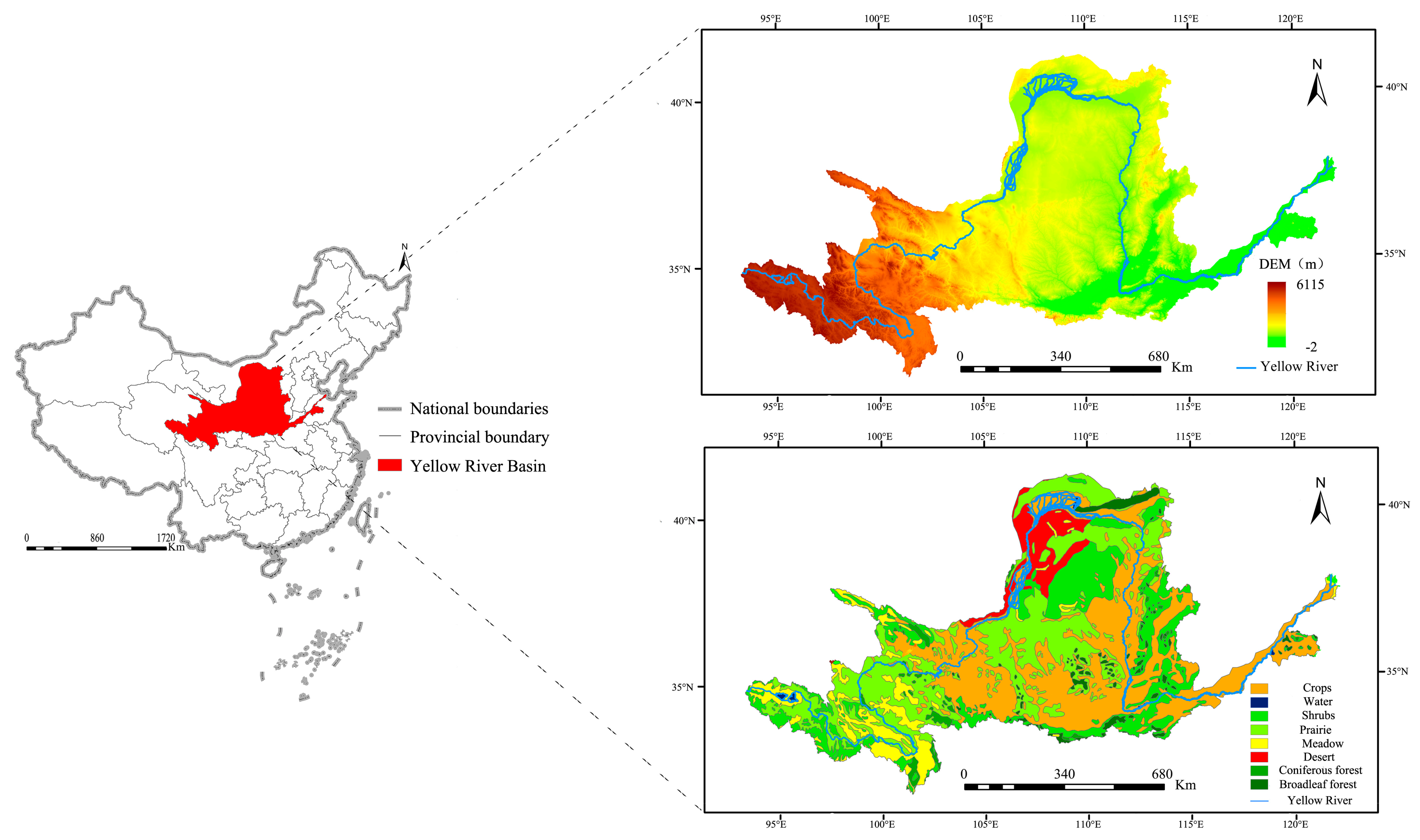
The Yellow River is the fifth longest river in the world. It has a total length of 5464 km and an altitudinal difference of 4444 m. The area of the YRB is 79.5 × 10⁴ km2, and it has a continental climate with an annual mean precipitation of 534 mm and an annual mean temperature varying in turn from northwest to southeast in the range of 2–4 °C. The diverse landform types within the basin have facilitated the development of various vegetation types. Within the study area, agricultural crops, grasslands and savannah bushes, shrubs and coppice forests, meadows and marshes, deserts, broadleaf forests, coniferous forests, and non-vegetated areas account for 34.86%, 28.79%, 18.78%, 7.39%, 5.20%, 2.64%, 1.77%, 0.57% of the total land area, respectively (Figure 1).
2.2. Data Sources
2.2.1. Remote Sensing Data of the Normalized Difference Vegetation Index (NDVI)
The United States National Aeronautics and Space Administration has developed highly accurate Global Inventory Modeling and Mapping Studies (GIMMS) NDVI datasets [34]. In this study, the GIMMS NDVI 3g V1.0 datasets for 1982–2015 were selected to ensure data continuity and consistency. The spatial and temporal resolutions of the data are 8 km and 15 days, respectively. The NDVI data for the entire study duration were merged month by month using the maximum value composites method [35]. Abnormal data (non-vegetated areas) in the datasets were removed.
2.2.2. Meteorological Data
All data on the monthly mean temperature (T), maximum monthly mean temperature (Tmax), minimum monthly mean temperature (Tmin), precipitation (R), and sunshine duration were acquired from the daily datasets of the country’s terrestrial climate data (V3.0) published on the China Meteorological Data Network (http://data.cma.cn/). These datasets contain daily data recorded by the 824 national reference and basic climatological stations. The highest temperature occurs around 2 p.m., and the lowest temperature occurs around 2 a.m., so the highest and lowest temperatures can be used to indicate daytime and nighttime temperatures. Considering the lack of data from solar radiation stations, the amounts of solar radiation were calculated using sunshine duration. Next, standard and reasonable methods [36,37] were used to compile the various monthly data, followed by spatial interpolation of the meteorological factors using ANUSPLIN [38,39].
2.2.3. Vegetation Data
This study utilized maps of China’s vegetation cover at a scale of 1:1 million published by the Cold and Arid Regions Science Data Center, Chinese Academy of Sciences (CAS) [40]. Considering the impact of accurate vegetation categorization on the research findings, the Reclass function of ArcGIS 10.1 was used to divide the YRB’s vegetation covers into seven main categories: (i) Broadleaf forests, (ii) coniferous forests, (iii) meadows and marshes, (iv) shrubs and coppice forests, (v) agricultural crops, (vi) grasslands and savannah bushes, and (vii) deserts.
3. Research Method and Models
3.1. The modified CASA Model for Calculating NPP
NPP is the basis for using the remote sensing method to study NEP. The starting point for the CASA model is the vegetation’s physiological processes, which are combined with climatic conditions of the vegetation growth regions to build an NPP estimation model [41]. However, this model is based solely on the vegetation types found in North America. Given the large variations between different regions in the world, the YRB’s NPP was estimated using an improved CASA model by Zhu [42,43], which is more applicable to China’s climate and vegetation. Zhu’s model determines NPP using two variables: the vegetation’s absorbed photosynthetic active radiation (APAR) and solar energy utilization rate (ε).
where x is the spatial position; t is time; NPP(x,t) denotes the NPP of pixel x at time t (gC·m−2·a−1); APAR denotes the APAR of pixel x at time t (MJ·m−2·a−1); and ε(x,t) denotes the actual solar energy utilization rate of pixel x at time t (gC·MJ−1).
The vegetation’s APAR is dependent on the total amount of solar radiation and the vegetation’s ability to utilize solar radiation. The equations are as follows [44]:
The FPAR and NDVI could be linearly correlated and their linearity is determined by the FPARmax and FPARmin which are corresponded to the NDVImax and NDVImin [45,46,47].
There is also a strong linearity between FPAR and SR [48,49,50].
where SOL(x,t) denotes the total amount of solar radiation received by pixel x at time t (MJ·m−2·t−1); FPAR(x,t) and FPAR(x,t) SR are the vegetation absorption rates of incident photosynthetically active radiation derived from NDVI and SR, respectively. The constant 0.5 indicating the ratio of effective solar radiation used by the vegetation to the total amount of solar radiation [43]; NDVIi,max and NDVIi,min denote the maximum and minimum NDVI values of the ith type of vegetation, respectively; SR(x,t) denotes the SR value of pixel x at time t; SRi,max and SRi,min denote the maximum and minimum SR values of the ith type of vegetation; and FPARmax and FPARmin denote the maximum and minimum values of the fraction of photosynthetically active radiation (FPAR) [51] which are 0.950 and 0.001, respectively [52].
The FPAR values derived from NDVI are greater than ground truths, while the FPAR derived from NDVI are smaller than ground truths with fewer differences. In order to minimize the “distance” between FPAR and ground truth data, we used the average FPAR estimated from both NDVI and SR [50].
FPAR(x,t) is the vegetation absorption rate of incident photosynthetically active radiation.
The solar energy utilization rate (ε) is jointly affected by temperature and soil moisture and has a direct impact on the fixed NPP amount. The calculation equations are as follows:
where Tε1(x,t) and Tε2(x,t) are the temperature stress coefficients; Wε(x,t) is the water stress coefficient; and ε* is the vegetation’s maximum solar energy utilization rate under ideal conditions.
where Topt(x) denotes the mean temperature of the month in which the maximum NDVI for a specific region is reached within a year. The value of Tε1 is 0 if the mean temperature of a particular month is ≤10 °C.
For a particular month, if its mean temperature T(x,t) is 10 °C higher or 13 °C lower than the optimum temperature, the Tε2 value of that month is equal to 50% of the value when =.
where PET(x,t) denotes the potential evapotranspiration amount (mm) and EET(x,t) denotes the estimated evapotranspiration amount (mm). Both PET and EET are treated as 0 when the monthly mean temperature is ≤0 °C. In this situation, the Wε(x,t) of that month is equal to the value of the previous month, meaning that Wε(x,t) = Wε(x,t-1).
3.2. Calculation of NEP
NEP can be understood as the difference in value between the NPP and the amount of CO2 emission through soil microbial respiration, without considering the impact of other natural and anthropogenic factors. It can be calculated using the equation [53]:
where NEP and NPP are the vegetation’s net ecosystem productivity and net primary productivity, respectively, and RSM is soil microbial respiration. When NEP > 0, the amount of CO2 being sequestered by the vegetation is larger than that emitted by the soil. Positive and negative values denote carbon sinks and sources, respectively.
Based on the findings of past studies [54], the equation for calculating the amount of soil microbial respiration is as follows:
where T is the monthly mean temperature and R is the amount of precipitation.
3.3. Analysis of NEP Changes
Based on the estimation of NEP, the trend analysis model, a stability analysis model and Hurst index model based on R/S analysis were used to study the time scale change, spatial stability analysis and future change trend of vegetation carbon sink. The second-order partial correlation analysis of the pixel by pixel is used to analyze the response of vegetation carbon sink under the asymmetry of daytime and nighttime.
3.3.1. Model for Slope Analysis
Univariate linear regression analysis reflects the linear relationship between a dependent variable and an independent variable. [55] This method can eliminate the impact of abnormal factors during slope analysis of NEP, thereby, ensuring that the evolutionary trend of NEP over a long time series is accurately reflected. Its calculation equation is as follows:
where Slope is the slope of the linear fitting equation, NEPi is the NEP value of the ith year obtained using the maximum value composites method, and n is the duration of the study period.
3.3.2. Model for Stability Analysis (CV)
The coefficient of variation reflects the degree of dispersion among the random variables in terms of the unit mean value. It was selected to measure and evaluate the stability of the NEP time series [56]. Its equation is:
where CV represents the coefficient of variation, is the mean value, and σ is the standard deviation. A largevalue indicates that the data are more dispersed, and highly volatile and unstable over time. In the opposite scenario, data distribution is concentrated, and data stability is good.
3.3.3. Hurst Exponent Model Based on R/S Analysis
Time series with long-term dependencies are ubiquitous in nature. The Hurst exponent can quantitatively describe the long-term dependence of NEP in a time series (Table 1) [57]. The basic principle is as follows: for times t1, t2, …, tn, the corresponding response time series is assumed to be μ1, μ2, …, μn; for any positive integer τ ≥ 1, the average of the time series is:
The cumulative deviation with X(t) is expressed as:
For every τ, the difference between the corresponding maximum X(t) and minimum X(t) is termed the range, which is denoted as:
The standard deviation used by Hurst is:
3.4. Partial Correlation Analysis between the Nep and Climatic Factors
Since the NEP is jointly affected by multiple meteorological factors, the coefficient obtained using traditional correlation analysis is unable to simply explain the impact of a meteorological factor. In other words, the singular impact of a factor cannot be distinguished when the factors are mutually related. As such, second-order partial correlation analysis was used in this study. Specifically, the impact of two meteorological factors on the NEP was controlled to analyze the response of the NEP to variations in a third meteorological factor. In so doing, the strength of the correlation can be determined while being free of interference. The second-order partial correlation is calculated using the first-order partial correlation coefficient. In order to obtain the latter, it is necessary to first calculate the correlation coefficient using the equation [58]:
The equation for calculating the first-order partial correlation coefficient is:
The equation for calculating the second-order partial correlation coefficient is:
where xi, yi are the elements for partial correlation calculation;, are the mean values of elements x, y, respectively; 1, 2 are the control variables; rxy., rxy·1, and rxy·12 are the correlation coefficient, first-order partial correlation coefficient, and second-order partial correlation coefficient of elements x, y, respectively; rx·1 and ry·1 are the correlation coefficients of x,1 and y,1, respectively; and rx2·1 and ry2·1 are the first-order partial correlation coefficient of x,2 and y,2, respectively.
The t-test is generally used to determine the significance of the partial correlation coefficients. The statistical equation for this test is: [59]
where r is the partial correlation coefficient, n is the number of samples, and q is the number of degrees of freedom.
4. Results and Discussion
4.1. Comparative Analysis of the YRB’s Diurnal Asymmetric Warming and NPP
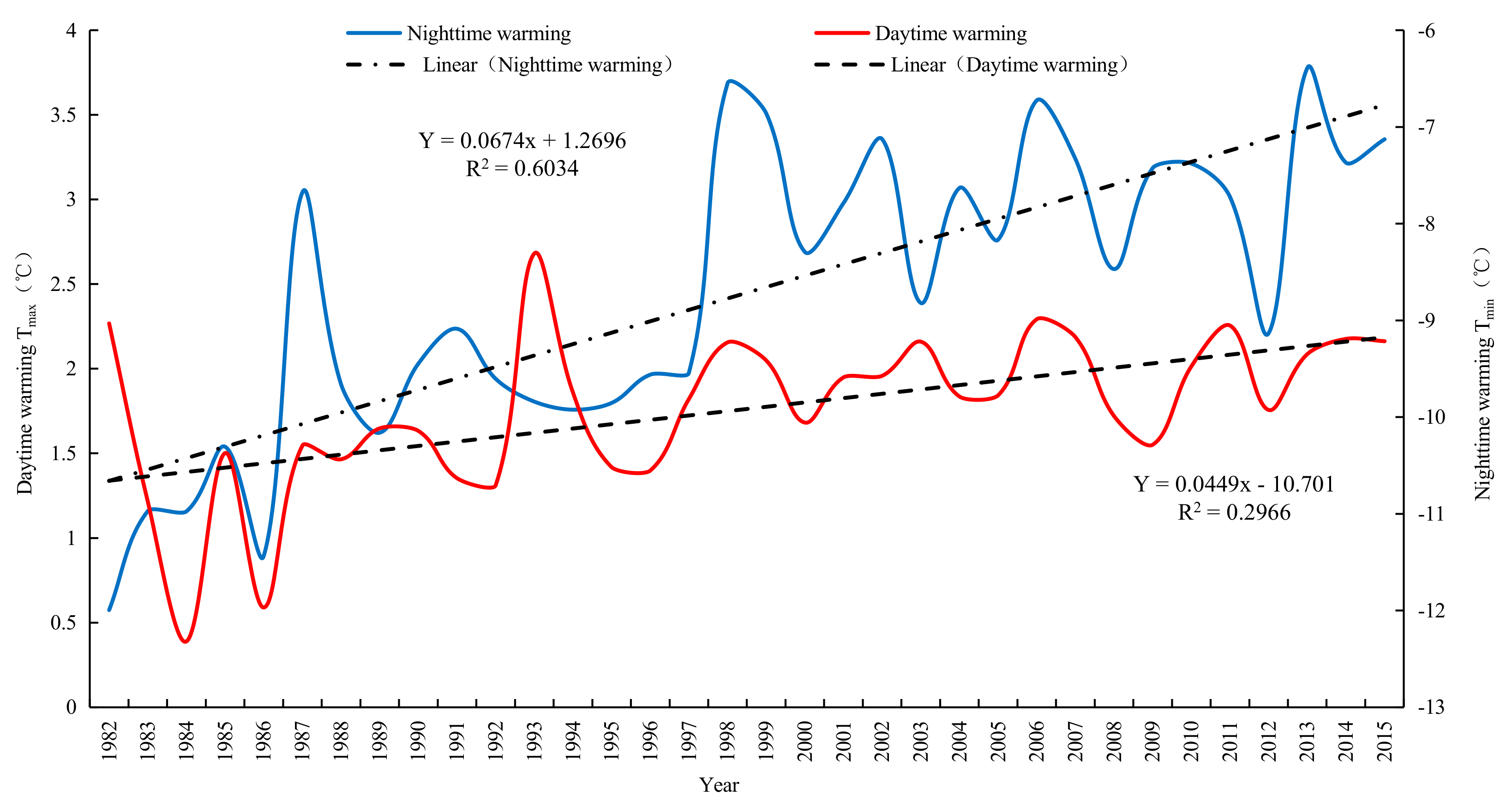
For the YRB, both its daytime warming (Tmax) and nighttime warming (Tmin) exhibited upward trends from 1982 to 2015 (Figure 2). Based on the fitting model, the Tmin and Tmax in Yellow River basin increased 0.0674 °C and 0.0449 °C respectively every 10 years. A significant and positive correlation existed between Tmax and Tmin, with the correlation coefficient being 0.55 (P < 0.1). It indicates that the temperature increased faster in nighttime than in daytime in the Yellow River basin. Diurnal asymmetric warming was obvious. In addition, the upward trend of Tmin was significantly higher than that of Tmax, with the rate of increase of the former being 1.50 times that of the latter (1.4 and 1.5 times according to Solomon [60] and Zhao [32], respectively). In the context of unbalanced temperature changes between daytime and nighttime, we investigated the influences of terrestrial vegetation in the carbon sink dynamic. On this basis, we will carry out research on the changes of vegetation carbon sink function under the asymmetry of day and night warming in the Yellow River Basin.
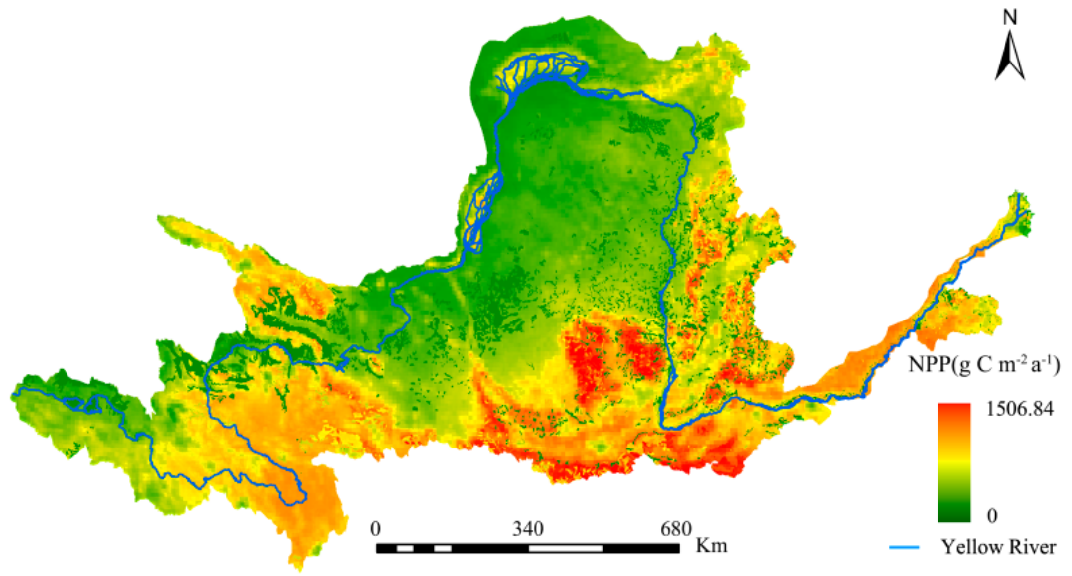
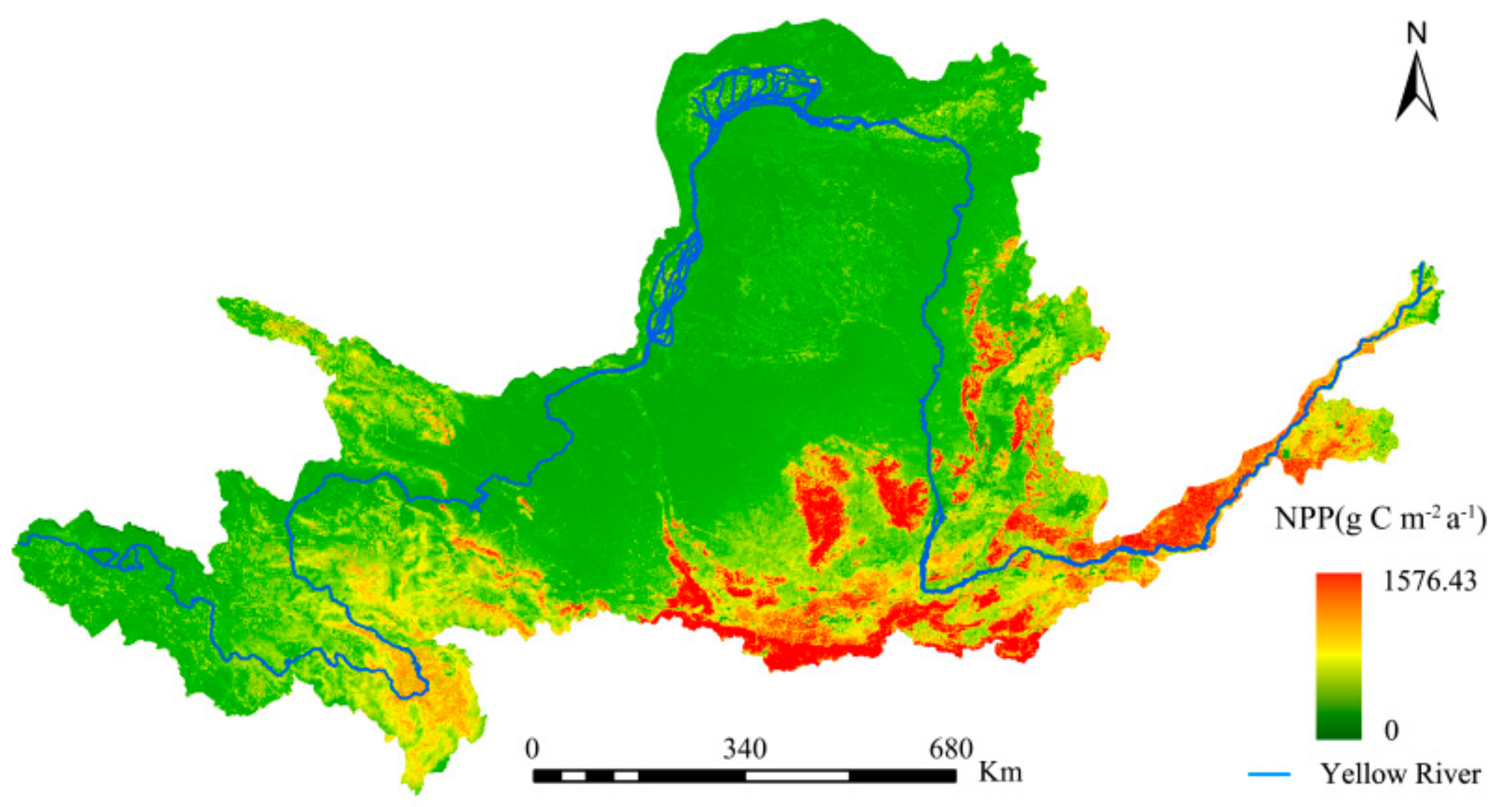
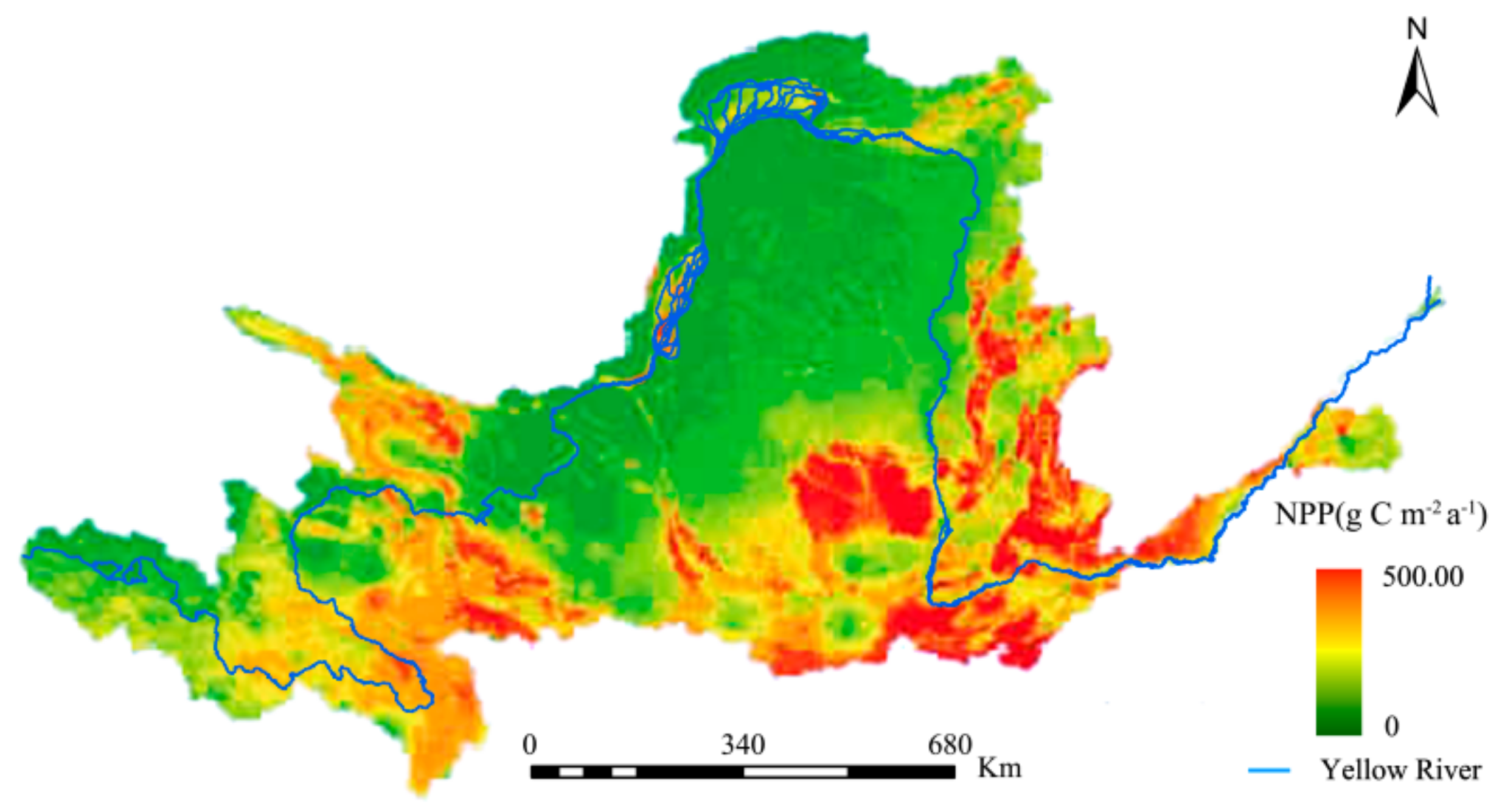
A comparison was made between the NPP estimated by this study and past studies to illustrate the accuracy of the former. Specifically, comparisons were made between this study’s NPP estimates (Figure 3) and those of the Resources and Environmental Science Data Center (RESDC), and the research findings of Chen et al. [61] for the same study area (Figure 4 and Figure 5, respectively).
The spatial distributions of the YRB’s NPP was consistent for the three studies. The maximum difference in the estimates between Figure 3 and Figure 4 did not exceed 60 g C·m−2·a−1, with the NPP changes from 2000 to 2010 being consistent. This study’s NPP estimates were also significantly higher when Figure 3 and Figure 5 were compared. Overall, the interpolation method used in this study was more accurate and had wider solar radiation coverage, making it more plausible.
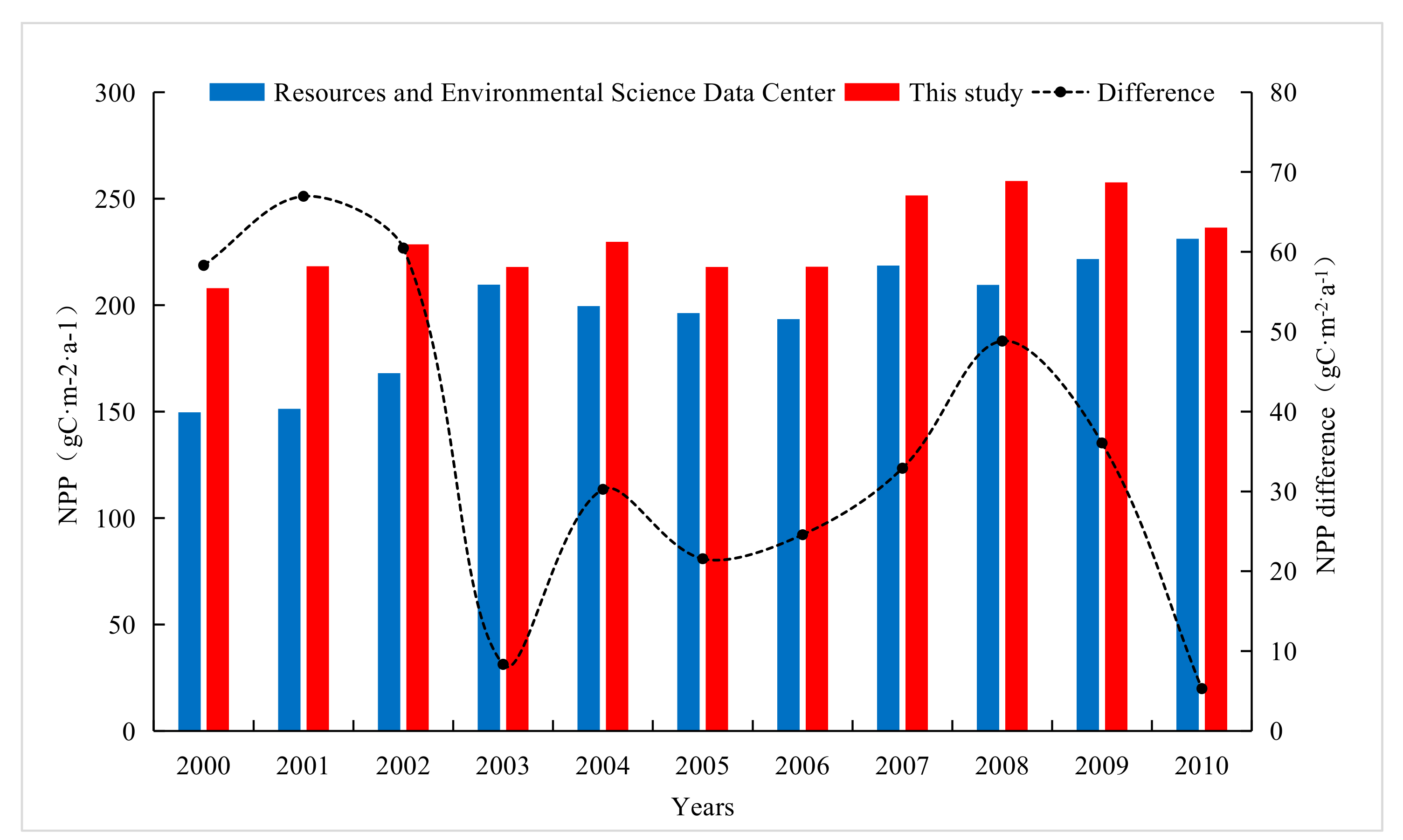
Since the time series of NPP estimation data of the Resource and Environmental Science Data Center is 2000–2010, the NPP estimation results of the same period were intercepted and compared. As can be seen from Figure 6, the results of this study are higher than the NPP estimates of the Resource and Science Data Center. The average values of 2000–2010 are 231.10 g C·m−2·a−1 and 195.32 g C·m−2·a−1, respectively, with a difference of 35.78 g C·m−2·a−1. The NPP of the Resource and Environmental Sciences Data Center was estimated by GLM_PEM model, while the CASA model was used in this study. Considering the limiting effect of temperature and water on the potential utilization of light energy, it is considered that the limiting effect of temperature and water follows the minimum factor rule of ecology, that is, the ultimate environmental limitation depends on the environmental factors with the strongest stress. Therefore, the estimation result is more accurate, and is more widely used in the global NPP estimation [62].
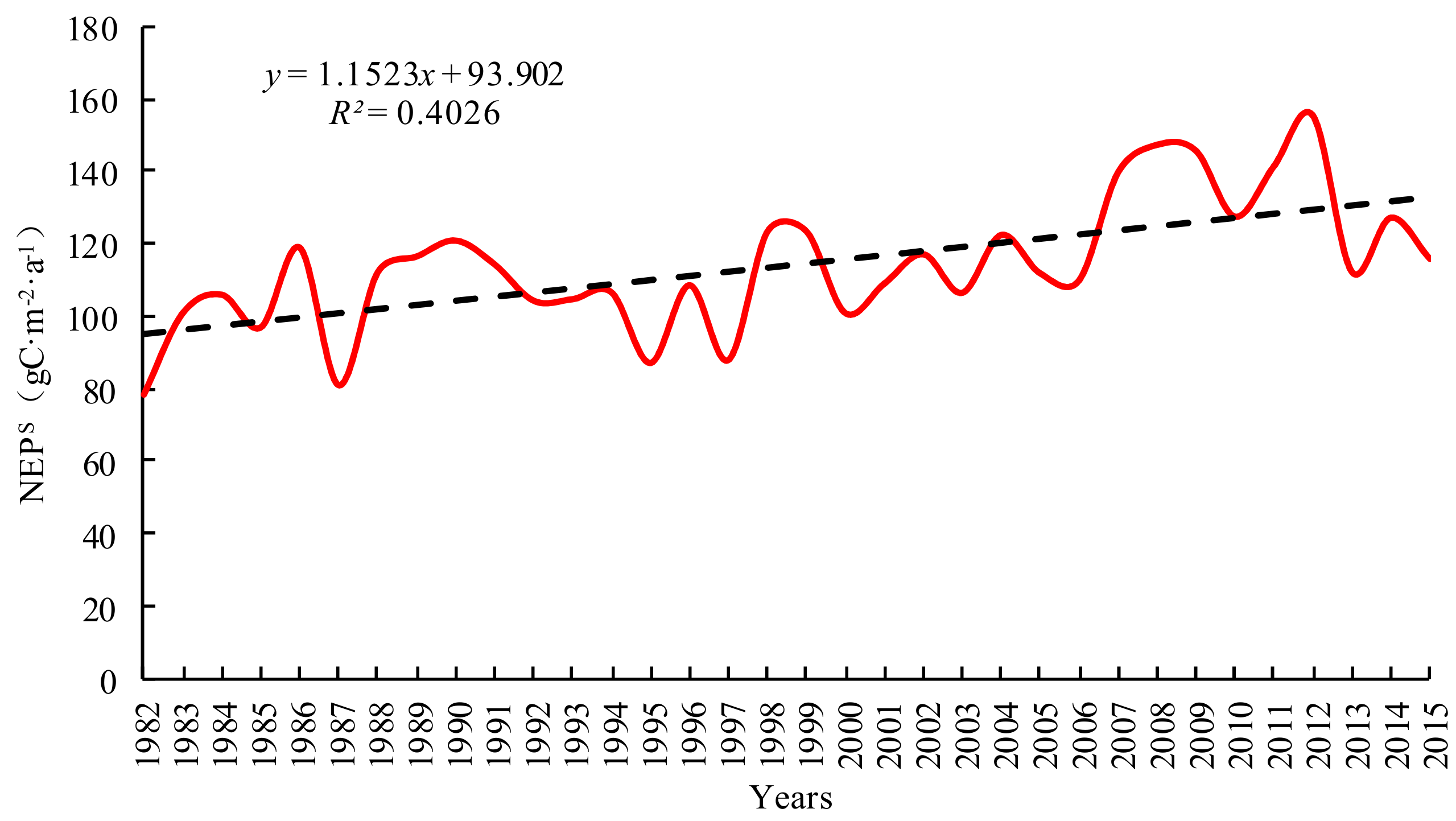
Heterogeneity in the distribution of the YRB’s vegetation causes great spatiotemporal changes in the resultant carbon sequestration capacities. With the aforementioned NPP estimates as the base, changes in the YRB’s NEP over time were calculated according to Equations (11) and (12). The results are shown in Figure 7. From 1982 to 2015, fluctuations in the YRB’s carbon sequestration capacities exhibited an overall upward trend. The annual minimum and maximum mean carbon sequestration amounts were recorded in 1982 and 2012, at 78.24 and 155.33 g C·m−2·a−1, respectively.
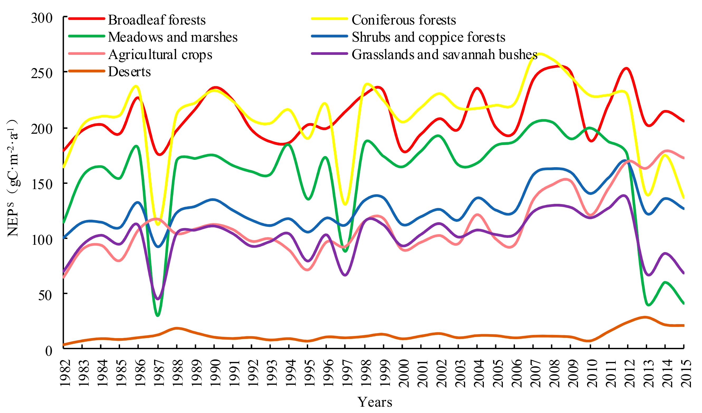
There were differences in carbon sequestration amounts by the YRB’s different vegetation types (Figure 8). The types and amounts, arranged in descending order, are as follows: (i) broadleaf forest (210.28 gC·m−2·a−1), (ii) coniferous forest (208.75 gC·m−2·a−1), (iii) meadow and marsh (155.43 gC·m−2·a−1), (iv) shrub and coppice forest (126.99 gC·m−2·a−1), (v) agricultural crop (113.25 gC·m−2·a−1), (vi) grassland and savannah bush (100.76 gC·m−2·a−1), and (vii) deserts (12.27 gC·m−2·a−1). The strong carbon sink function of broadleaf forest is also suggested by existing literature [63]. In addition, the amount of carbon sink of forest is much higher than agricultural crops and grassland [64,65].
The NEP is an important indicator of carbon sequestration by a region’s vegetation. The spatial distribution of NEP from the YRB vegetation cover from 1982 to 2015 was calculated according to Equations (10) and (11) and is shown in Figure 9. This NEP of Inner Mongolia grassland is validated with 1000 soil heterotrophic respiration samples [66]. The convincing validation results support the NEP accuracy. In addition, the comparison between different NEP models verified the spatial uniformity of NEP in the study area [67]. The values were higher in the western and southeastern regions. The former is predominantly mountainous with high altitudes and the main vegetation types (forests and grasslands) have good carbon sequestration capacities; the latter has an extensive distribution of cultivated land and a relatively large area of forested land, endowing it with relatively good carbon sequestration capacities. The northern region of the study area has lower NEP values mainly because the natural environmental conditions are relatively poor; with the predominance of deserts and plateaus, the degree of vegetation cover is relatively low. Consequently, its carbon sequestration capacity is also significantly lower than that of the other regions.
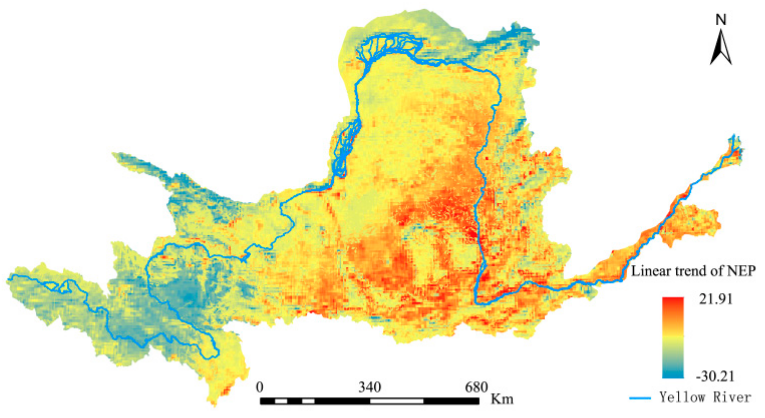
Based on a univariate linear regression analysis and the maximum composite data for the YRB’s annual NPP from 1982 to 2015, the ArcGIS 10.1 software was used to visualize spatial changes in the annual mean NEP within the study area (Figure 10). There was a general trend of slow increases over the study period; areas with increases and decreases accounted for 60.21% and 31.49% of the total area, respectively. The former was mainly distributed in the YRB’s southeastern region, while the latter was mainly located in the upper reaches of the Yellow River. There were relatively few areas where the NEP remained unchanged. These included the high-altitude mountainous areas and areas with low vegetation coverage, accounting for only 8.30% of the total area.
The coefficient of variation for the annual mean NEP was calculated according to Equation (13) and is shown in Figure 11. The overall spatial distribution pattern showed high values in the northern region and low values in the southern region. Low fluctuations were predominant while high fluctuations mainly occurred in the YRB’s northern region, where the vegetation coverage varied greatly over the study period, the impacts of anthropogenic activities were clearer, and the overall stability of the vegetation’s carbon sequestration capacity was poor. Nevertheless, the coefficient of variation for the majority of the study area was 3% or less, indicating that the NEPs were relatively stable as a whole.
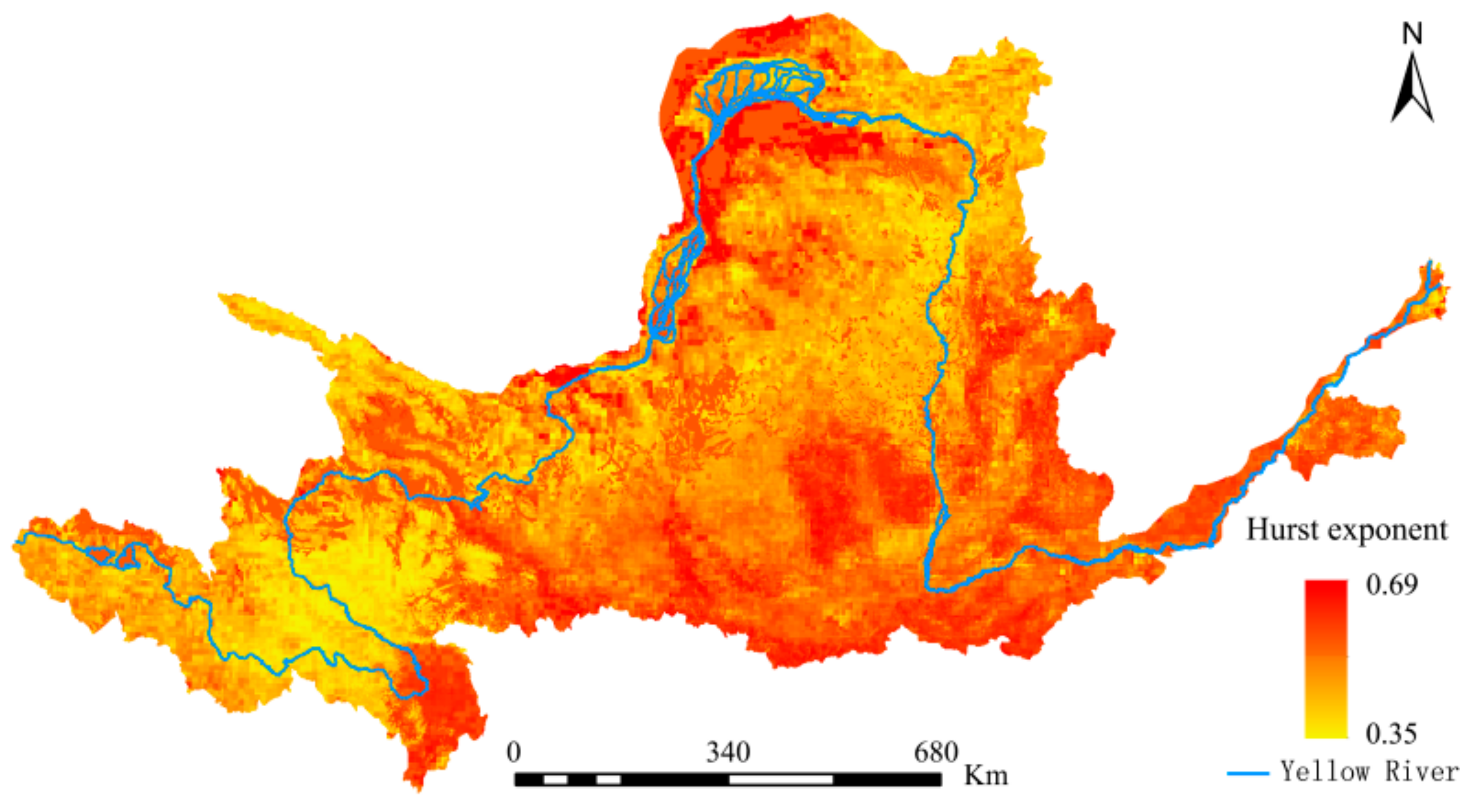
Following the ‘pattern–process’ analysis described above, the Hurst exponent was introduced to further explore potential future trends in the YRB’s NEP (Figure 12). The mean Hurst exponent for the YRB’s NEP was 0.52, with a range of 0.35–0.69. The Hurst exponent for 59.49% of the total area was greater than 0.5, while that for the balance 40.51% was smaller than 0.5. These indicate that for the YRB’s NEP, changes in the same direction were more dominant than those in the opposite direction.
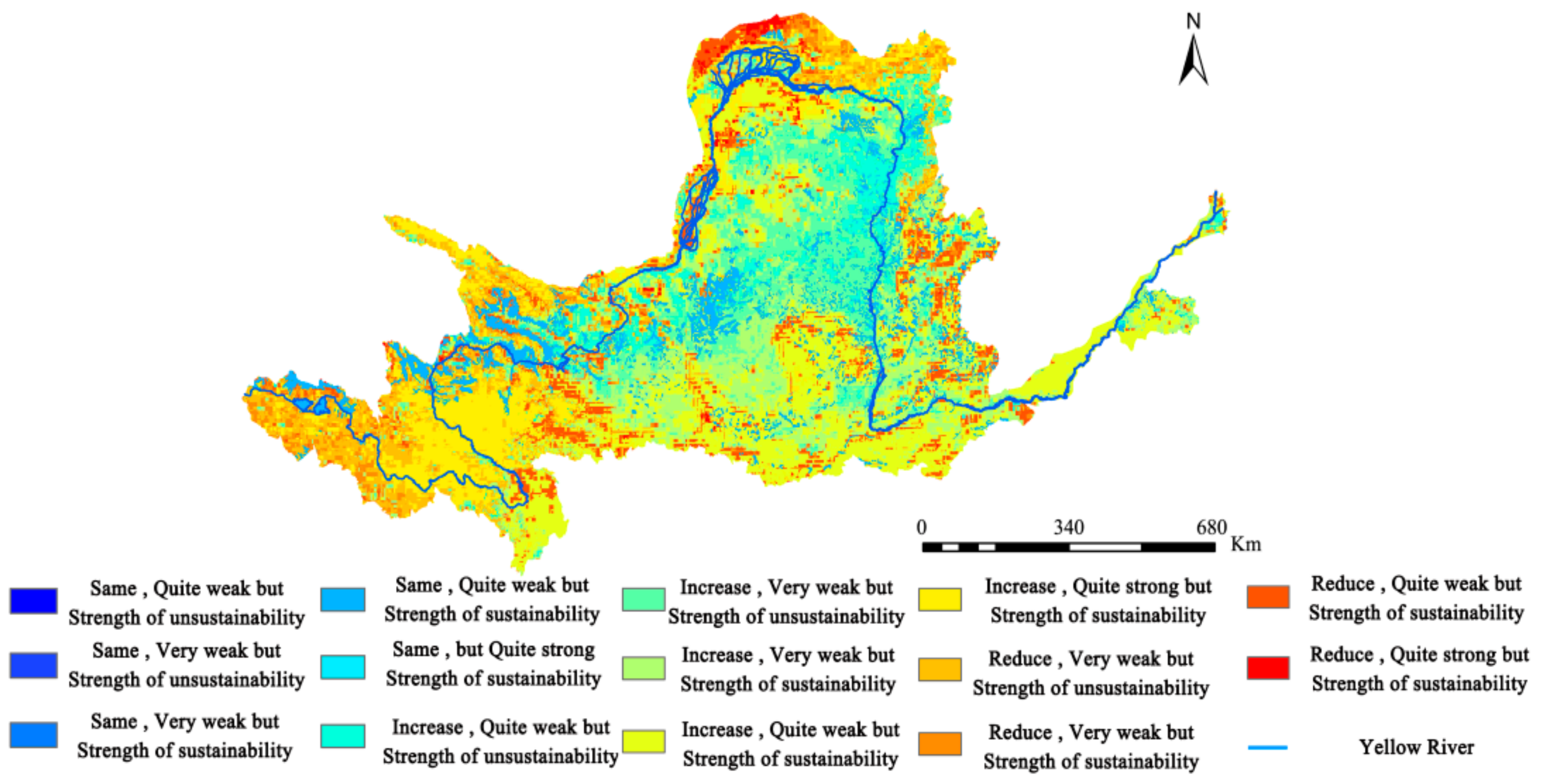
The results for the trend in NEP changes were superimposed onto those from the Hurst exponent for analysis, from which the coupling characteristics of the trend and continuity in the YRB’s NEP changes were obtained (Figure 13). This study divided the coupling characteristics into 14 situations. Among these, the proportions of the YRB’s total land area being under four situations are as follows (in descending order): (i) weak but increasing sustainability (21.89%), (ii) weak but increasing unsustainability (15.75%), (iii) very weak but increasing sustainability (15.58%), and (iv) quite strong and increasing sustainability (11.74%). This result indicates that there was no significant change in the distribution of the YRB’s NEP from 1982 to 2015 and that sustainability was relatively poor.
It should be noted that areas with the same and weak sustainability accounted for 8.30% of the YRB’s total area. These are mainly distributed in the YRB’s western region, representing the basin’s headwater area, where vegetation cover is fragile. Given the poor sustainability of these areas, action should be taken to prevent the degradation of vegetation covers. Governance of ecological environments must also be strengthened.
4.2. Response of the YRB’s NEP to Diurnal Asymmetric Warming
Most of the regions in the YRB have an arid or semi-arid climate, with precipitation being one of the main factors limiting vegetation growth. Hence, precipitation was used as the control variable during second-order partial correlation analysis to calculate the correlations of Tmax and Tmin with NEP. The partial correlation coefficient of Tmax and Tmin with NEP of different vegetation types was shown in Table 2.
The correlations of Tmax and Tmin with NEP are not significant. On one hand, except grassland and meadow and marsh, the Tmax is positively correlated with NEP of other vegetation covers with minimal significance. On the other hand, except broadleaf forest, Tmin has slight positive correlation NEP of with other vegetation covers. The different responses of different vegetation to diurnal temperature increase lie in physiological variations of vegetation. The increase of Tmin may increase vegetation productivity by reducing the frequency of frost occurrence [68]. This may lead to a positive partial correlation between NEP and Tmin in some vegetation. Previous studies have shown that water use efficiency at different levels in typical grasslands of northern China has a specific response to daytime and night warming. Warming during the day reduced the water use efficiency of the ecosystem by 5.66% [69]. Therefore, the increasing of Tmax modifies the way that water is utilized in meadows and herbaceous swamp vegetation, further restraining the growth of vegetation. The increase of Tmin exacerbates autotrophic breath of meadow and marsh and steppe at night. As a result, the compensation would improve their productivity. The partial correlation between Tmin and various vegetation types in the study area did not pass the significance test, indicating that the response of NEP to diurnal and night warming of different vegetation types was not significant. The partial correlation between Tmin and NEP is not significant, which is consistent with previous research results [70,71,72]. Except for meadow and herbaceous swamp, Tmax shows positive correlations with NEP of other vegetation. Meanwhile, except for broad-leaved forest, Tmin shows positive correlations with NEP of other vegetation. The difference of the response of different vegetation types to the diurnal warming is mainly due to the difference of the physiological structure and the environmental response strategy of different vegetation. The increasing of Tmin increases the spontaneous respiration in the broadleaf forest at night, further accelerating the consumption of photosynthate. This process would have negative impacts on the growth and development of broad-leaved forest. Moreover, the negative correlation between the meadow and the herb marsh on the Tmax is due to the difference in the utilization strategy of the vegetation type to water resources. The increasing of Tmin gives rise to the nighttime autotrophic respiration of meadow and steppe, and the consequent compensation would increase their productivity [73]. Crops have a more positive response to daytime warming, daytime warming is conducive to increasing photosynthetic intensity of crops, thereby increasing the accumulation of organic matter; while night warming plays a role in promoting crops, but the positive correlation is not significant, which is consistent with previous research results [32].
The difference between the vegetation physiological process and different resource utilization strategies is one of the main reasons for the different response of vegetation to day and night warming. However, the different natural environments of vegetation growth is another important reason for the different response of vegetation to day and night warming. The calculation of the second-order partial correlation coefficient between the grid-by-grid NEP and day–night warming is helpful to express the spatial distribution of vegetation and day-night warming more intuitively, so as to formulate reasonable protection policies for different regions. The spatial distribution of partial correlation coefficients between maximum and minimum temperatures and NEP is shown in Figure 14 and Figure 15.
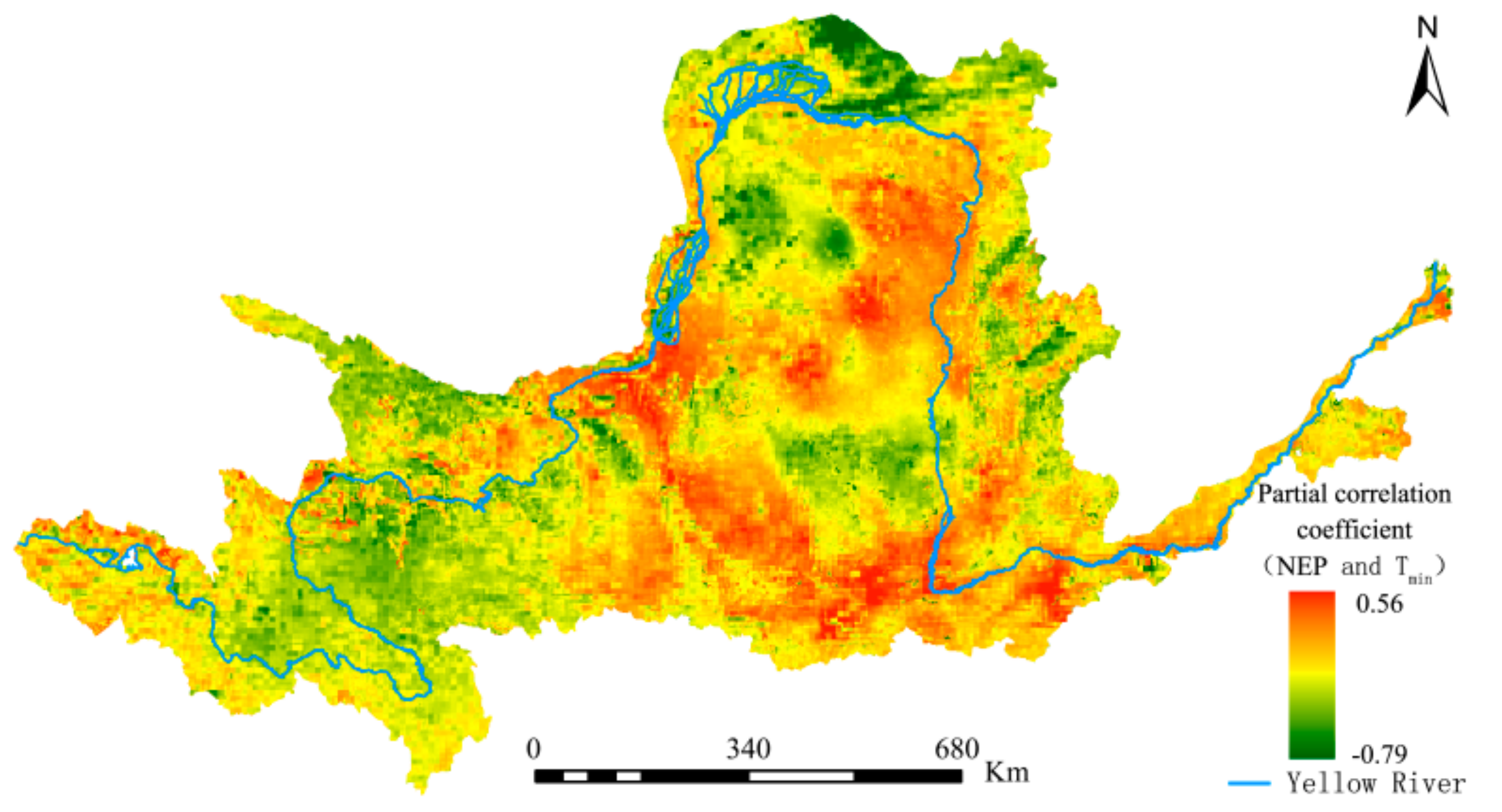
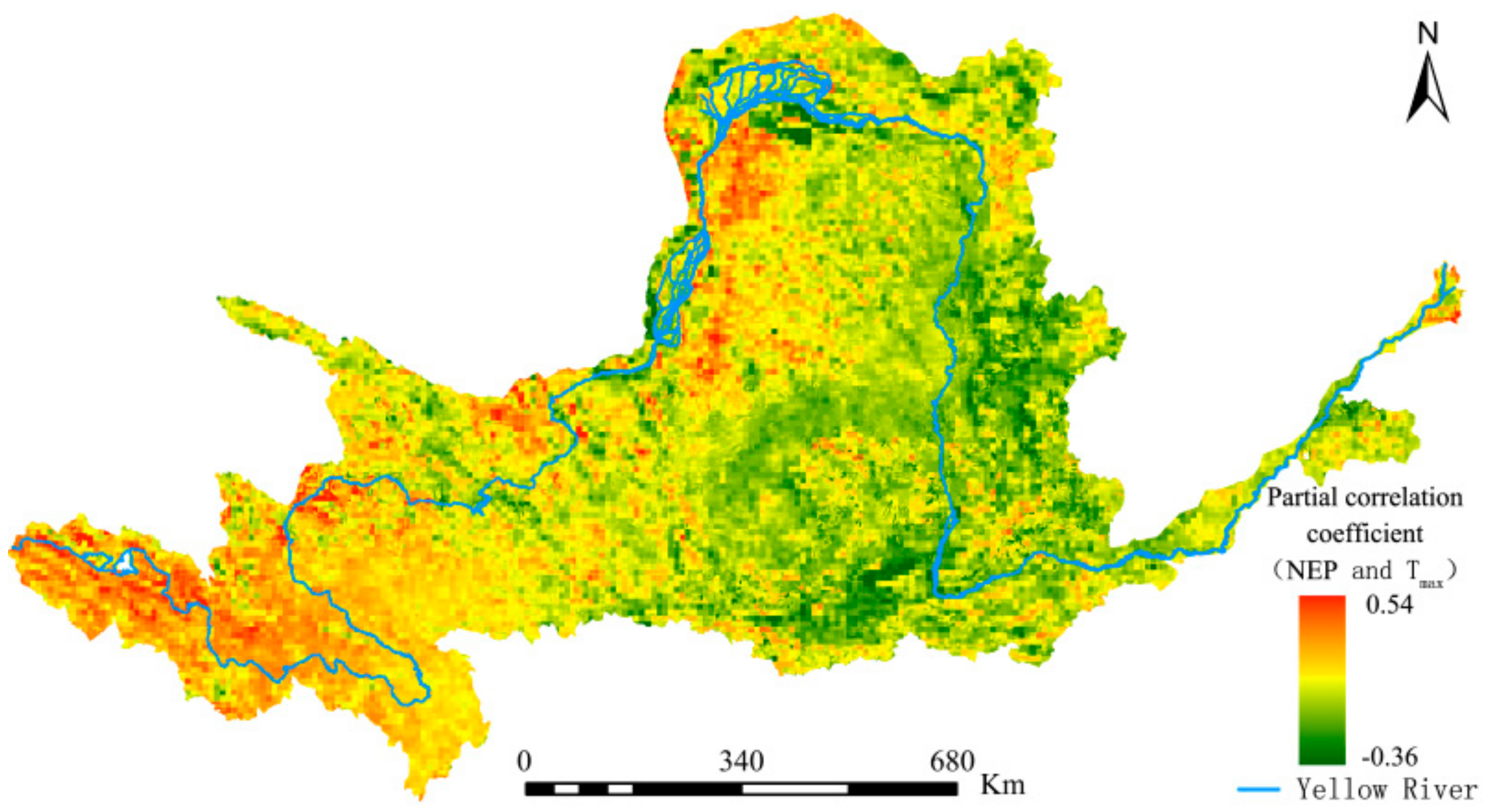
It can be seen from Figure 13 that significant spatial differences exist in terms of the impacts of diurnal warming on the YRB’s vegetation carbon sequestration capacity, with both showing opposite spatial distribution trends. Under constant precipitation and Tmax, approximately 48.37% and 51.63% of the regions in the YRB had positive and negative correlations between NEP and Tmin, respectively. However, when precipitation and Tmin remained unchanged (Figure 15), approximately 67.51% and 32.49% of the regions had positive and negative correlations between NEP and Tmax, respectively. The proportion of regions in the YRB’s total area that passed the significance test was calculated. The results show that areas with a partial correlation between NEP and Tmin that had passed the significance test exceeded those with a partial correlation between NEP and Tmax by 3.89%. This finding confirms that nighttime temperature changes in the YRB have had more extensive impacts on vegetation cover.
5. Conclusions
Protection of the vegetation cover in China’s YRB is an issue of global concern. The YRB’s NPP from 1982 to 2015 was estimated using a combination of multiple models. The soil microbial respiration model was also used to determine the study area’s NEP and its spatiotemporal distributions. The study’s findings are as follows:
- The YRB experienced obvious diurnal asymmetric warming from 1982 to 2015, with the rate of increase for Tmin being 1.50 times that of Tmax. The total NPP showed an overall linear upward trend with large inter-annual fluctuations. In terms of spatial distribution, the YRB’s NPP exhibited a pattern of high spatial differentiation, with low values in the northern region and high values in western and southeastern regions.
- Temporal variations of the YRB’s NEP were characterized by upward fluctuations. There were substantial variations in NEP between the various vegetation types in the following order: broadleaf forests > coniferous forests and meadows and marshes > shrubs and coppice forests > agricultural crops > grasslands and savannah bushes > deserts. For temporal fluctuations of NEP arising from different vegetation types, the characteristics were similar. Spatially, NEP values were highest in western and southeastern regions of the YRB, and lowest in the northern region. Overall, the NEP within the basin were relatively stable.
- There were significant spatial differences in terms of the impacts of diurnal warming on the YRB’s vegetation carbon sequestration capacity, which were enhanced by daytime warming but significantly inhibited by nighttime warming. The numbers of areas with nighttime warming that passed significance testing were slightly higher than those with daytime warming.
During the study period, NEP changes in the same direction were significantly stronger than that in the opposite direction. Although there was no significant change in the distribution of NEP, sustainability was generally poor. Therefore, future developments of the YRB should focus on the recovery of vegetation cover and governance of the ecological environments in the headwater area.
NEP is jointly affected by the natural environment and anthropogenic activities; however, in this study, only the impacts of temperature and precipitation on the YRB’s NEP were discussed. Anthropogenic factors, such as a region’s economic development, were not considered. In future studies, a comprehensive analysis should be made by incorporating correlations between anthropogenic activities and the NEP. In addition, there is a time lag when it comes to the impact of meteorological factors on vegetation growth, which differs depending on the region and meteorological factor involved.
Using a mathematical model to simplify the complex ecosystem process is conducive to a more intuitive understanding of the simple ecosystem operation process, and easy to adjust the future development of the ecosystem. However, the measured data can more truly reflect the changes of an ecosystem to a certain extent, so combining the measured data with the mathematical model can more scientifically and accurately reflect the actual situation of NEP in the Yellow River Basin. In order to study, we will focus on the acquisition of measured data, and based on the measured data to establish the ecosystem carbon cycle function evaluation index suitable for the actual situation of the study area, and focus on the heterogeneity of NEP between different regions.
Thus, future studies must also examine the time-lag effect of meteorological factors on NEP. The findings of this study can serve as a reference for the protection of vegetation covers in drainage basins, as well as for regions in Asia, South America, and Northern Europe with developmental experiences that are similar to that of the study area.
Author Contributions
All authors conceived, designed, and implemented the study. P.Z. and J.H. designed and carried out the study. W.J. participated in the analysis and presentation of analytic results. Y.Y. contributed the data used in this study.
Funding
This paper was supported by the National Natural Science Foundation of China (41601175, 41801362). The key scientific research project of the Henan province (16A610001), supported by the Program for Innovative Research Team (in Science and Technology) in University of Henan Province (16IRTSTHN012), the GDAS’ Project of Science and Technology Development (2017GDASCX-0101, 2018GDASCX-0904), and the Guangdong Innovative and Entrepreneurial Research Team Program (2016ZT06D336). Its content does not represent the official position of the Chinese government and is entirely the responsibility of the authors.
Conflicts of Interest
All authors declare no conflict of interest.
References
- IPCC. Climate Change 2014: Impacts, Adaptation, and Vulnerability; Cambridge University Press (IPCC Secretariat): Cambridge, UK, 2014. [Google Scholar]
- Schuur, E.A.G.; McGuire, A.D.; Schädel, C.; Grosse, G.; Harden, J.W.; Hayes, D.J.; Hugelius, G.; Koven, C.D.; Kuhry, P.; Lawrence, D.M.; et al. Climate change and the permafrost carbon feedback. Nature 2015, 520, 171–179. [Google Scholar] [CrossRef] [PubMed]
- Solow, A.R. Global warming: A call for peace on climate and conflict. Nature 2013, 497, 179–180. [Google Scholar] [CrossRef] [PubMed]
- Hoegh, G.O.; Bruno, J.F. The impact of climate change on the world’s marine ecosystems. Science 2010, 328, 1523–1528. [Google Scholar] [CrossRef] [PubMed]
- Cook, J.; Oreskes, N.; Doran, P.T.; Anderegg, W.R.L.; Verheggen, B.; Maibach, E.W.; Carlton, J.S.; Lewandowsky, S.; Skuce, A.G.; Green, S.A. Consensus on consensus: A synthesis of consensus estimates on human-caused global warming. Environ. Res. Lett. 2016, 11, 048002. [Google Scholar] [CrossRef]
- Ang, B.W.; Su, B. Carbon emission intensity in electricity production: A global analysis. Energy Policy 2016, 94, 56–63. [Google Scholar] [CrossRef]
- Liu, Z.; Guan, D.; Wei, W.; Davis, S.J.; Ciais, P.; Bai, J.; Peng, S.S.; Zhang, Q.; Hubacek, K.; Marland, G.; et al. Reduced carbon emission estimates from fossil fuel combustion and cement production in China. Nature 2015, 524, 335–338. [Google Scholar] [CrossRef] [PubMed] [Green Version]
- Wise, M.; Dooley, J.; Luckow, P.; Calvin, K.; Kyle, P. Agriculture, land use, energy and carbon emission impacts of global biofuel mandates to mid-century. Appl. Energy 2014, 114, 763–773. [Google Scholar] [CrossRef]
- Shuai, C.; Shen, L.; Jiao, L.; Wu, Y.; Tan, Y.T. Identifying key impact factors on carbon emission: Evidences from panel and time-series data of 125 countries from 1990 to 2011. Appl. Energy 2017, 187, 310–325. [Google Scholar] [CrossRef]
- Schimel, D.; Pavlick, R.; Fisher, J.B. Observing terrestrial ecosystems and the carbon cycle from space. Glob. Chang. Biol. 2015, 21, 1762–1776. [Google Scholar] [CrossRef] [PubMed]
- Schimel, D.; Stephens, B.B.; Fisher, J.B. Effect of increasing CO2 on the terrestrial carbon cycle. Proc. Natl. Acad. Sci. USA 2015, 112, 436–441. [Google Scholar] [CrossRef] [PubMed]
- Friend, A.D.; Lucht, W.; Rademacher, T.T.; Asner, G.P.; Saatchi, S.; Townsend, P.; Miller, C.; Frankenberg, C.; Hibbard, K.; Cox, P. Carbon residence time dominates uncertainty in terrestrial vegetation responses to future climate and atmospheric CO2. Proc. Natl. Acad. Sci. USA 2014, 111, 3280–3285. [Google Scholar] [CrossRef] [PubMed]
- Reyer, C.; Lasch-Born, P.; Suckow, F.; Gutsch, M.; Murawski, A.; Pilz, T. Projections of regional changes in forest net primary productivity for different tree species in Europe driven by climate change and carbon dioxide. Ann. For. Sci. 2014, 71, 211–225. [Google Scholar] [CrossRef]
- Seaquist, J.W.; Olsson, L.; Ouml, J.A. A remote sensing-based primary production model for grassland biomes. Ecol. Model. 2003, 169, 131–155. [Google Scholar] [CrossRef]
- Lieth, H.; Whittaker, R.H. (Eds.) Primary Productivity of the Biosphere; Springer: New York, NY, USA, 1975; p. 274. [Google Scholar]
- Melillo, J.M.; McGuire, A.D.; Kicklighter, D.W.; Moore, B.; Vorosmarty, C.J.; Schloss, A.L. Global climate change and terrestrial net primary production. Nature 1993, 363, 234. [Google Scholar] [CrossRef]
- Nemani, R.R.; Keeling, C.D.; Hashimoto, H.; Jolly, W.M. Climate-driven increases in global terrestrial net primary production from 1982 to 1999. Science 2003, 300, 1560–1563. [Google Scholar] [CrossRef] [PubMed]
- Field, C.B.; Behrenfeld, M.J.; Randerson, J.T.; Falkowski, P. Primary production of the biosphere: Integrating terrestrial and oceanic components. Science 1998, 281, 237–240. [Google Scholar] [CrossRef] [PubMed]
- Running, S.W.; Nemani, R.R.; Heinsch, F.A.; Zhao, M.; Reeves, M.; Hashimoto, H. A Continuous Satellite-Derived Measure of Global Terrestrial Primary Production. BioScience 2004, 54, 547–560. [Google Scholar] [CrossRef]
- Reeves, M.C.; Moreno, A.L.; Bagne, K.E.; Running, S.W. Estimating climate change effects on net primary production of rangelands in the United States. Clim. Chang. 2014, 126, 429–442. [Google Scholar] [CrossRef] [Green Version]
- Nicholson, E.M. The Conservation programme of the international biological programme (IBP). Polar Record 1969, 14, 760–764. [Google Scholar] [CrossRef]
- An, N.; Price, K.; Blair, J. Estimating above-ground net primary productivity of the tallgrass prairie ecosystem of the Central Great Plains using AVHRR NDVI. Int. J. Remote Sens. 2013, 34, 3717–3735. [Google Scholar] [CrossRef]
- Potter, C.S.; Randerson, J.T.; Field, C.B.; Matson, P.A.; Vitousek, P.M.; Mooney, H.A.; Klooster, S.A. Terrestrial ecosystem production: a process model based on global satellite and surface data. Glob. Biogeochem. Cycles 1993, 7, 811–841. [Google Scholar] [CrossRef]
- Hicke, J.A.; Asner, G.P.; Randerson, J.T. Satellite-derived increases in net primary productivity across North America, 1982–1998. Geophys. Res. Lett. 2002, 29, 1–4. [Google Scholar] [CrossRef]
- Nayak, R.K.; Patel, N.R.; Dadhwal, V.K. Estimation and analysis of terrestrial net primary productivity over India by remote-sensing-driven terrestrial biosphere model. Environ. Monit. Assess. 2010, 170, 195–213. [Google Scholar] [CrossRef] [PubMed]
- Zhang, S.W.; Zhang, R.; Liu, T.; Song, X.; Adams, M.A. Empirical and model-based estimates of spatial and temporal variations in net primary productivity in semi-arid grasslands of Northern China. PLoS ONE 2017, 12, e0187678. [Google Scholar] [CrossRef]
- Liu, Z.D.; Li, B.; Fang, X.; Tucker, C.; Los, S.; Birdsey, R.; Jenkins, J.C.; Field, C.; Holland, E. Dynamic characteristics of forest carbon storage and carbon density in the Hunan Province. Acta Ecol. Sin. 2016, 36, 6897–6908. (In Chinese) [Google Scholar] [CrossRef]
- Huang, C.D.; Zhang, J.; Yang, W.Q.; Tang, X.; Zhao, A.J. Dynamics on forest carbon stock in Sichuan and Chongqing city. Acta Ecol. Sin. 2008, 28, 966–975. (In Chinese) [Google Scholar] [CrossRef]
- Pan, J.H.; Huang, K.J.; Li, Z. Spatio-temporal variation in vegetation net primary productivity and its relationship with climatic factors in the Shule River basin from 2001 to 2010. Acta Ecol. Sin. 2017, 37, 1888–1899. [Google Scholar] [CrossRef]
- Mao, D.H.; Wang, Z.M.; Han, J.X.; Ren, C.Y. Spatio-temporal pattern of net primary productivity and its driven factors in Northeast China in 1982–2010. Sci. Geogr. Sin. 2012, 32, 1106–1111. (In Chinese) [Google Scholar] [CrossRef]
- Zhu, Z.; Piao, S.L.; Myneni, R.B.; Huang, M.T.; Zeng, Z.Z.; Canadell, J.G.; Ciais, P.; Sitch, S.; Friedlingstein, P.; Arneth, A.; et al. Greening of the Earth and its drivers. Nat. Clim. Chang. 2016, 6, 791–795. [Google Scholar] [CrossRef] [Green Version]
- Zhao, J.; Liu, X.J.; Du, Z.Q.; Wu, Z.T.; Xu, X.M. Effects of the asymmetric diurnal-warming on vegetation dynamics in Xinjiang. China Environ. Sci. 2017, 37, 2316–2321. (In Chinese) [Google Scholar]
- Bates, D.; Lindstrom, M.; Wahba, G. Gcvpack-routines for generalized cross validation. Commun. Stat. Simul. Comput. 1987, 16, 263–297. [Google Scholar] [CrossRef]
- Kobayashi, H.; Dye, D.G. Atmospheric conditions for monitoring the long-term vegetation dynamics in the Amazon using normalized difference vegetation index. Remote. Sens. Environ. 2005, 97, 519–525. [Google Scholar] [CrossRef]
- Guo, N.; Zhu, Y.J.; Wang, J.M.; Deng, C.P. The relationship between NDVI changes and climatic factors in different types of vegetation in Northwest China over the past 22 years. Chin. J. Plant Ecol. 2008, 32, 319–327. (In Chinese) [Google Scholar] [CrossRef]
- China Meteorological Administration. Standard for Ground Meteorological Observation; GBT352212017; Meteorology Press: Beijing, China, 2003. (In Chinese)
- China Meterological Administration. People’s Republic of China Meteorological Industry Standard (QX/T 22-2004); Ground climate data for 30 years and its statistical methods; QXT222004; China Meterological Administration: Beijing, China, 2007. (In Chinese)
- Tan, J.B.; Li, A.N.; Lei, G.B. Contrast on Anusplin and Cokriging meteorological spatial interpolation in southeastern margin of Qinghai-Xizang Plateau. Plateau Meteorol. 2016, 35, 875–886. (In Chinese) [Google Scholar] [CrossRef]
- Ren, X.; Zheng, J.H.; Mu, C.; Yan, K.; Xu, Y.B. Reliability evaluation of different meteorological interpolation methods in the NPP estimation of grassland in Xinjiang. Pratac. Sci. 2017, 3, 439–448. (In Chinese) [Google Scholar] [CrossRef]
- China Academy of Sciences (Chinese Academy of Sciences) Editorial Board of Vegetation Map. 1:1000000 Vegetation Atlas of China; Science Press: Beijing, China, 2001. (In Chinese) [Google Scholar]
- Potter, C.S. Terrestrial biomass and the effects of deforestation on the global carbon cycle: Results from a model of primary production using satellite observations. Bioscience 1999, 49, 769–778. [Google Scholar] [CrossRef]
- Zhu, W.Q. Remote Sensing Estimation of Net Primary Productivity of Vegetation in China Land Ecosystem and Its Relationship with Climate Change. Ph.D. Thesis, Beijing Normal University, Beijing, China, 2005. (In Chinese). [Google Scholar]
- Zhu, W.Q.; Chen, Y.Y.; Xu, D.; Li, J. Advances in terrestrial net primary productivity (NPP) estimation models. Chin. J. Ecol. 2005, 24, 296–300. (In Chinese) [Google Scholar] [CrossRef]
- Piao, S.L.; Fang, J.Y.; Guo, Q.H. Using CASA model to estimate the net primary productivity of vegetation in China. Chin. J. Plant Ecol. 2001, 25, 603–608. (In Chinese) [Google Scholar] [CrossRef]
- Ruimy, A.; Saugier, B.; Dedieu, G. Methodology for the estimation of terrestrial net primary production from remotely sensed data. J. Geophys. Res.-A 1994, 99, 5263–5283. [Google Scholar] [CrossRef]
- Sellers, P.J. Canopy reflectance, photosynthesis, and transpiration, II. The role of biophysics in the linearity of their interdependence. Int. J. Remote Sens. 1992, 6, 1335–1372. [Google Scholar] [CrossRef]
- Huemmrich, K.F.; Goward, S.N. Spectral vegetation indexes and the remote sensing of biophysical parameters. IGARSS 1992, 2, 1017–1019. [Google Scholar] [CrossRef]
- Field, C.B.; Randerson, J.T.; Malmström, C.M. Global net primary production: Combining ecology and remote sensing. Remote Sens. Environ. 1995, 51, 74–88. [Google Scholar] [CrossRef] [Green Version]
- Los, S.O.; Justice, C.O.; Tucker, C.J. A global 1 by 1 NDVI data set for climate studies derived from the GIMMS continental NDVI data. Int. J. Remote Sens. 1994, 15, 3493–3518. [Google Scholar] [CrossRef]
- Sellers, P.J.; Randall, D.A.; Collat, G.J.; Berry, J.A.; Field, C.B. A revised land surface parameterization (SiB2) for atmospheric GCMS. Part I: Model formulation. J. Clim. 1996, 9, 706–737. [Google Scholar] [CrossRef]
- Zhu, W.Q.; Pan, Y.Z.; He, H.; Yu, D.Y.; Hu, H.B. Simulation of maximum light utilization rate of typical vegetation in China. Chin. Sci. Bull. 2006, 51, 700–706. [Google Scholar] [CrossRef]
- Zhu, W.Q.; Pan, Y.Z.; Zhang, J.S. Estimation of net primary productivity of land vegetation using remote sensing in China. Chin. J. Plant Ecol. 2007, 31, 413–424. (In Chinese) [Google Scholar] [CrossRef]
- Houghton, R.A. Terrestrial sources and sinks of carbon inferred from terrestrial data. Tellus B 1996, 48, 420–432. [Google Scholar] [CrossRef]
- Woodwell, G.M.; Whittaker, R.H.; Reiners, W.A.; Delwiche, C.C.; Botkin, D.B. The biota and the world carbon budget. Science 1978, 199, 141–146. [Google Scholar] [CrossRef] [PubMed]
- Stow, D.; Daeschner, S.; Hope, A.; Douglas, D.; Petersen, A.; Mynemy, R.; Zhou, L.; Oechel, W. Variability of the seasonally integrated normalized difference vegetation index across the north slope of Alaska in the 1990s. Int. J. Remote Sens. 2003, 24, 1111–1117. [Google Scholar] [CrossRef]
- Pizzo, H.P.; Ettenger, R.B.; Gjertson, D.W.; Reed, E.F.; Zhang, J.H.; Gritsch, A.; Tsai, E.W. Sirolimus and tacrolimus coefficient of variation is associated with rejection, donor-specific antibodies, and nonadherence. Pediat. Nephrol. 2016, 31, 2345–2352. [Google Scholar] [CrossRef] [PubMed]
- Hurst, H.E. Long term storage capacity of reservoirs. ASCE Trans. 1951, 116, 770–808. [Google Scholar] [CrossRef]
- Dasgupta, S.; Tyler, S.; Srinivasan, R.; Grossman, E.D. Functional Connectivity of Co-localized Brain Regions during Biological Motion, Face and Social Perception using Partial Correlation Analysis. J. Vis. 2014, 14, 1011. [Google Scholar] [CrossRef]
- Kenett, D.Y.; Tumminello, M.; Madi, A.; Gershgoren, G.G.; Mantegna, R.N.; Ben-Jacob, E. Dominating clasp of the financial sector revealed by partial correlation analysis of the stock market. PLoS ONE 2010, 5, 15032. [Google Scholar] [CrossRef] [PubMed] [Green Version]
- IPCC. Climate Change 2007: The Physical Science Basis. Contribution of Working Group I to the Fourth Assessment Report of the Intergovernmental Panel on Climate Change; Cambridge University Press (IPCC Secretariat): Cambridge, UK, 2007. [Google Scholar]
- Yuan, W.P.; Liu, S.G.; Yu, G.R. Global estimates of evapotranspiration and gross primary production based on MODIS and global meteorology data. Remote Sens. Environ. 2010, 114, 1416–1431. [Google Scholar] [CrossRef] [Green Version]
- Chen, Q.; Chen, Y.H.; Wang, M.; Jiang, W.G.; Hou, P.; Li, Y. Change of vegetation net primary productivity in Yellow River watersheds from 2001 to 2010 and its climatic driving factors analysis. Chin. J. Appl. Ecol. 2014, 25, 2811–2818. (In Chinese) [Google Scholar] [CrossRef]
- Gong, J.; Zhang, Y.; Qian, C.Y. Temporal and spatial variation of net ecosystem productivity in the white Longjiang basin of Gansu. Acta Ecol. Sin. 2017, 37, 5121–5128. (In Chinese) [Google Scholar] [CrossRef]
- Pang, R.; Gu, F.X.; Zhang, Y.D.; Hou, Z.Y.; Liu, S.R. Temporal and spatial dynamics of net ecosystem productivity in alpine region of Southwest China. Acta Ecol. Sin. 2012, 32, 7844–7856. [Google Scholar] [CrossRef]
- Hu, B.; Sun, R.; Chen, Y.J.; Feng, L.C.; Sun, L. Estimation of the Net Ecosystem Productivity in Huang-Huai Hai Region Combining with Biome-BGC Model and Remote Sensing Data. J. Nat. Resour. 2011, 26, 2061–2071. (In Chinese) [Google Scholar] [CrossRef]
- Lobell, D.B. Changes in diurnal temperature range and national cereal yields. Agric. For. Meteorol. 2007, 145, 229–238. [Google Scholar] [CrossRef]
- Zhang, Q. Specific Response of Water Use Efficiency to Asymmetric Day-Night Warming in Typical Grasslands of Northern China. Master’s Thesis, Henan University, Henan, China, 2013. (In Chinese). [Google Scholar]
- Dai, E.F.; Huang, Y.; Wu, Z.; Zhao, D.S. Temporal and spatial patterns of carbon source/sink in grassland ecosystems in Inner Mongolia and their relationship with climatic factors. Acta Geogr. Sin. 2016, 71, 21–34. (In Chinese) [Google Scholar] [CrossRef]
- Yang, Y.Z.; Ma, Y.D.; Jiang, H.; Zhu, Q.A.; Liu, J.X.; Peng, C.H. Evaluating the carbon budget pattern of Chinese terrestrial ecosystem from 1960 to 2006 using Integrated Biosphere Simulator. Acta Ecol. Sin. 2016, 36, 3911–3922. (In Chinese) [Google Scholar] [CrossRef]
- Liang, C.L.; Yu, Q.Z.; Liu, Y.J.; Zhang, Z.L. Effect of day and night warming on NDVI of wetland vegetation in Nansi Lake. Trop. Geogr. 2015, 35, 422–436. (In Chinese) [Google Scholar] [CrossRef]
- Lovettdoust, J. Plant strategies, vegetation processes, and ecosystem properties. J. Veg. Sci. 2002, 13, 294–295. [Google Scholar] [CrossRef]
- Shi, F.S.; Wu, N.; Luo, P. Responses of plant community structure and biomass to subtropical alpine meadow in Northwest Sichuan. Acta Ecol. Sin. 2008, 28, 5286–5293. (In Chinese) [Google Scholar] [CrossRef]
- Wan, S.Q.; Xia, J.; Liu, W.; Niu, S. Photosynthetic overcompensation under nocturnal warming enhances grassland carbon sequestration. Ecology 2009, 90, 2700–2710. [Google Scholar] [CrossRef] [PubMed]
Figure 1.
Overview of the study area.

Figure 2.
Diurnal warming situation of the Yellow River Basin (YRB) from 1982 to 2015.

Figure 3.
Spatial distribution of the net primary productivity (NPP) from 2000 to 2010, as estimated by this study.
Figure 3.
Spatial distribution of the net primary productivity (NPP) from 2000 to 2010, as estimated by this study.

Figure 4.
Spatial distribution of NPP from 2000 to 2010, as estimated by the Resources and Environmental Science Data Center (RESDC).
Figure 4.
Spatial distribution of NPP from 2000 to 2010, as estimated by the Resources and Environmental Science Data Center (RESDC).

Figure 5.
Changes in the YRB’s NPP from 2001 to 2010 and analysis of NPP changes driven by meteorological factors (from [61]).
Figure 5.
Changes in the YRB’s NPP from 2001 to 2010 and analysis of NPP changes driven by meteorological factors (from [61]).

Figure 6.
Comparison between the NPP estimation data of the Resource and Environmental Science Data Center and the results in this study.
Figure 6.
Comparison between the NPP estimation data of the Resource and Environmental Science Data Center and the results in this study.

Figure 7.
Changes in the Yellow River Basin’s NEP from 1982 to 2015.

Figure 8.
Changes in the Yellow River Basin (YRB)’s NEP by vegetation type from 1982 to 2015.

Figure 9.
Spatial distribution of the Yellow River Basin (YRB)’s annual mean NEP from 1982 to 2015.
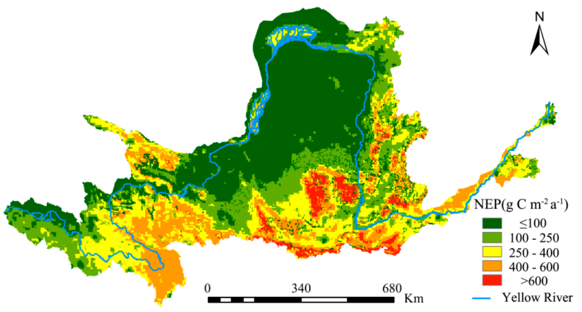
Figure 10.
Linear trends in the Yellow River Basin (YRB)’s NEP from 1982 to 2015.

Figure 11.
Degree of stability in changes of the Yellow River Basin (YRB)’s NEP from 1982 to 2015.
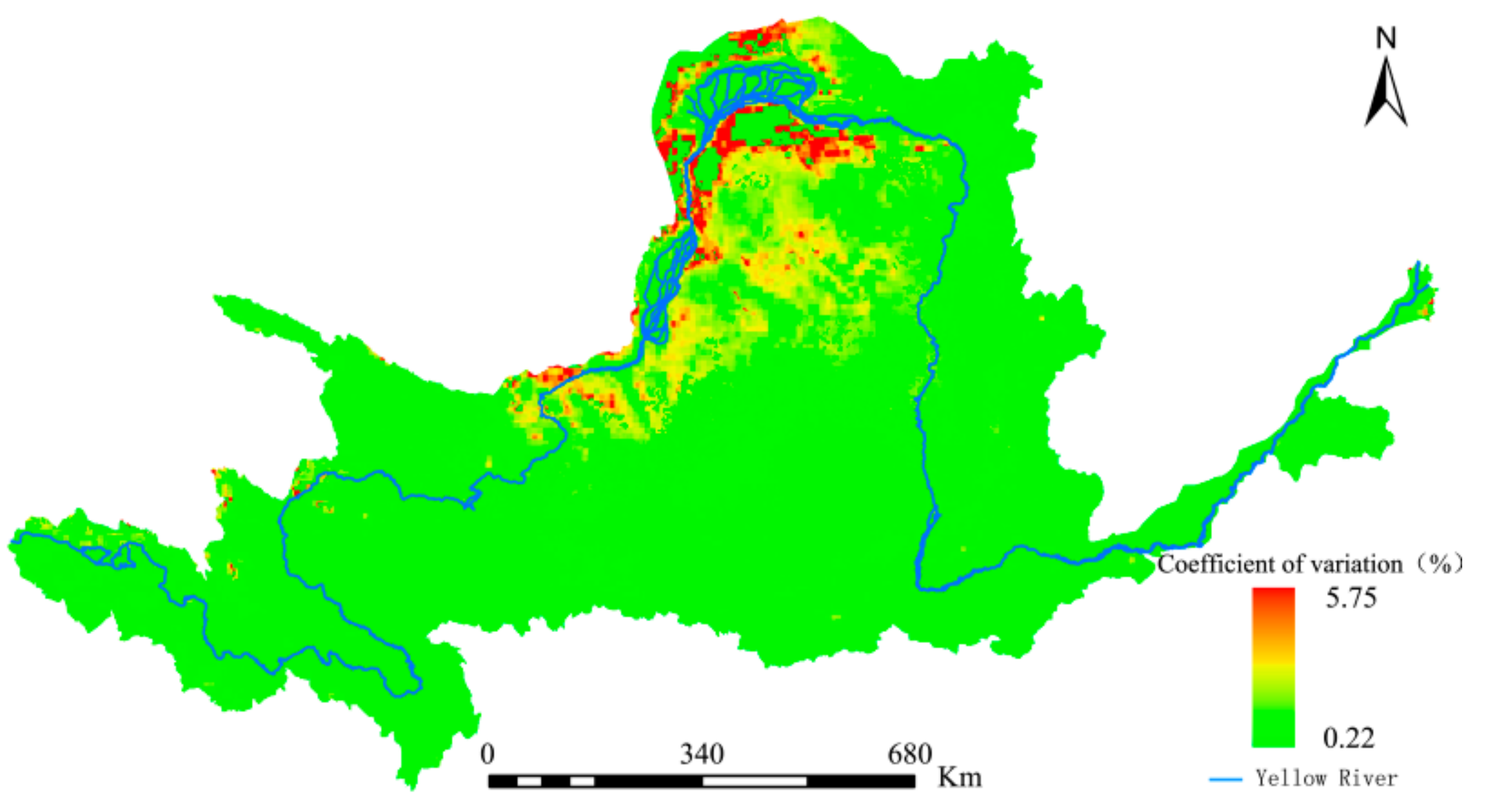
Figure 12.
Future trends in changes to the Yellow River Basin (YRB)’s NEP based on data from 1982 to 2015.
Figure 12.
Future trends in changes to the Yellow River Basin (YRB)’s NEP based on data from 1982 to 2015.

Figure 13.
Spatial distribution of changing characteristics of the Yellow River Basin (YRB)’s NEP from 1982 to 2015.
Figure 13.
Spatial distribution of changing characteristics of the Yellow River Basin (YRB)’s NEP from 1982 to 2015.

Figure 14.
Partial correlation coefficients between the Yellow River Basin (YRB)’s NEP and Tmin from 1982 to 2015.
Figure 14.
Partial correlation coefficients between the Yellow River Basin (YRB)’s NEP and Tmin from 1982 to 2015.

Figure 15.
Partial correlation coefficients between the Yellow River Basin (YRB)’s net NEP and Tmax from 1982 to 2015.
Figure 15.
Partial correlation coefficients between the Yellow River Basin (YRB)’s net NEP and Tmax from 1982 to 2015.


Table 1.
Grading based on the Hurst exponent.
| Grade | Range of Hurst Exponent | Strength of Sustainability | Grade | Range of Hurst Exponent | Strength of Unsustainability |
|---|---|---|---|---|---|
| 1 | 0.50 < H ≤ 0.55 | Very weak | −1 | 0.45 < H ≤ 0.50 | Very weak |
| 2 | 0.55 < H ≤ 0.65 | Quite weak | −2 | 0.35 < H ≤ 0.45 | Quite weak |
| 3 | 0.65 < H ≤ 0.75 | Quite strong | −3 | 0.25 < H ≤ 0.35 | Quite strong |
| 4 | 0.75 < H ≤ 0.80 | Strong | −4 | 0.20 < H ≤ 0.25 | Strong |
| 5 | 0.80 < H ≤ 1.00 | Very strong | −5 | 0.00 < H ≤ 0.20 | Very strong |
Note: Two decimals are reserved for the Hurst exponent and the intensity of net ecosystem productivity (NEP) time dependence is also classified. When Hurst exponent is equal to 0.50, it indicates weak strength of unsustainability.
Table 2.
Partial correlation coefficient of Tmax and Tmin with NEP.
| Vegetation Types | Tmax | Tmin |
|---|---|---|
| Broadleaf forests | 0.457 ** | –0.261 |
| Coniferous forests | 0.072 | 0.014 |
| Meadows and marshes | –0.005 | 0.011 |
| Shrubs and coppice forests | 0.381 * | 0.266 |
| Agricultural crops | 0.383 * | 0.163 |
| Grasslands and savannah Bushes | 0.195 * | 0.097 |
| Deserts | 0.323 | 0.101 |
Note: * was passed p < 0.05 statistically significant test; ** was passed p < 0.01 statistically significant test.
© 2018 by the authors. Licensee MDPI, Basel, Switzerland. This article is an open access article distributed under the terms and conditions of the Creative Commons Attribution (CC BY) license (http://creativecommons.org/licenses/by/4.0/).
Share and Cite
MDPI and ACS Style
He, J.; Zhang, P.; Jing, W.; Yan, Y. Spatial Responses of Net Ecosystem Productivity of the Yellow River Basin under Diurnal Asymmetric Warming. Sustainability 2018, 10, 3646. https://doi.org/10.3390/su10103646
AMA Style
He J, Zhang P, Jing W, Yan Y. Spatial Responses of Net Ecosystem Productivity of the Yellow River Basin under Diurnal Asymmetric Warming. Sustainability. 2018; 10(10):3646. https://doi.org/10.3390/su10103646
Chicago/Turabian StyleHe, Jianjian, Pengyan Zhang, Wenlong Jing, and Yuhang Yan. 2018. "Spatial Responses of Net Ecosystem Productivity of the Yellow River Basin under Diurnal Asymmetric Warming" Sustainability 10, no. 10: 3646. https://doi.org/10.3390/su10103646
Note that from the first issue of 2016, this journal uses article numbers instead of page numbers. See further details here.