Stochastic Transportation Network Considering ATIS with the Information of Environmental Cost

Abstract

The environment problem is a sustainable hot topic in the field of transportation research. With higher awareness of the environment problem, travelers tend to choose more environment friendly traffic modes and travel routes. However, for motor vehicle drivers, the environmental cost is an implicit cost, which is not easily perceived. With the help of the advanced traveler information system (ATIS), a fresh scheme was proposed to reduce the environmental cost of the transportation network, which incorporates the information of environmental cost into ATIS to guide drivers to choose more environment-friendly routes. To test the validity of the scheme, we adopted the theory of stochastic network user equilibrium to assign two classes of drivers on the transportation network and analyzed the impact on environmental cost after applying this scheme. Mathematically, a mixed stochastic user equilibrium (SUE) model was proposed to analyze this scheme. The corresponding algorithm was also proposed. Both the model and algorithm were tested in the numerical examples. Through the examples, the validity and feasibility of our proposed scheme were also identified. Our research provided some new ideas for traffic planners and managers to reduce environmental costs caused by traffic.

1. Introduction

The sustainable development of transportation systems is a major concern throughout the world, which is typically characterized in terms of three dimensions, including “economic, environmental, and social” [1]. However, due to the long-term neglect of the environmental problem, the rapid development of urban cities is at the expense of the environment. The transportation system is a critical component of sustainable development, and it plays an important role in social and economic connections in our daily life. Car dependency also contributes several negative effects to environmental problems [2], where traffic exhaust emissions have long been considered as the main source of air pollutants [3,4,5]. The International Council on Clean Transportation pointed out that transport consumes approximately 20% of global energy use and it is responsible for about 25% of global energy related carbon dioxide emissions, with 75% of these emissions due to road transport energy use [6,7]. The environmental problem caused by transport is an ongoing challenge for governments.

Owing to the impact of five main climate change agreements on the transportation industry since 1992, the evolution of environmental awareness has become a growing research trend [8]. Most countries have established vehicle emissions related standards to control vehicle exhaust emissions from the source [9,10]. For example, the United States was the first country to establish fuel economy standards for passenger vehicles after the 1970’s oil crisis. Moreover, some other countries such as China have moved forward to tighten greenhouse gas (GHG) or fuel economy standards in recent years. The implementation of these standards has proven to be amongst the most cost-effective tools in controlling oil demand and GHG emissions from motor vehicles [11]. However, with rapid urbanization in developing countries, increased motorized travel demand in the future is expected to continuously contribute great amounts of pollutants to the atmosphere [12]. Some researchers suggest that one of the most efficient ways is to encourage people to choose ‘go-green’ traffic modes, such as public transport and bicycles to satisfy their daily travel demands, while keeping the environmental expenses low [13]. For private vehicle travel, limiting use of gasoline vehicles and promoting new energy cars have recently become an emerging national concern. For example, electric vehicles are viewed as a long-term effective solution to reduce environment pollution and have enjoyed fast-growing adoption in recent years [14,15].

In the field of transportation research, the choice behavior of travelers in one trip can be generally divided into two steps. The first step is to choose the traffic modes, and the second one is to choose the travel routes. We note that all the measures mentioned above are all about how to reduce the environmental cost from the traffic modes. Recent research shows that the shortest route with minimum travel time cost is not equivalent to the green route with minimum environmental cost [16,17]. The objectives of minimizing travel time and vehicle emissions are often conflicting, because the rates of vehicle emissions do not change monotonically with average travel speed [18]. Through incorporating measures of environmental cost into the shortest path problem, some methods were proposed to find the so-called environment-friendly or green paths [19,20]. The aims of these researches are to help people choose more environment-friendly routes to reduce the environmental cost. However, the route choice behavior of travelers should be further taken into consideration. In other words, traffic managers should not only find the routes with minimum environmental cost, but also guide drivers to choose them.

Nowadays, rapid advances in internet information technology have provided various data collection methods, which can capture and store large amounts of multi-type traffic data. These basic data can strongly enhance the development of intelligent traffic systems (ITS). As an important component of ITS, ATIS are generally believed to be an effective tool to improve individuals travel efficiency and ease traffic congestion [21,22]. With the comprehensive utilization of big data, ATIS can capture more exact real-time road conditions and find multi-objective routes for travelers. In fact, travelers are more likely to rely on ATIS to make route choices. On the level of management, the government can better manage individual trips for certain strategic objectives with the help of ATIS. Specifically, if the environmental cost can be incorporated into the path finding process in ATIS, the environmental cost of the transportation network may be effectively reduced through providing drivers with green route guidance. It is this idea that motivates our research.

Based on the aforementioned analysis, many researches about transportation have paid attention to the environmental problem. The main work includes establishing vehicle emission related standards, developing low-emission vehicles, promoting green traffic modes, and so on. From the perspective of management, these researches only focus on the individuals green traffic mode and route choice, and they seldom analyze this problem at network level. Moreover, the important impact of ATIS on travelers route choice is unnoticed. We have considered incorporating environmental cost into ATIS to guide travelers’ route choice, and to analyze this problem at network level, which fill the gaps in the literature. The aim of our research was to propose such a new scheme to reduce the environmental cost in the scale of the transportation network, from the perspective of traffic management.

The main contributions of our research includes three aspects: (1) We proposed a fresh scheme based on the travelers’ route choice behavior to reduce the environmental cost of the transportation network; (2) We proposed a mixed SUE model and the corresponding algorithm to describe and solve this problem; (3) We tested the effectiveness of the scheme by applying the model and algorithm in the scale of the transportation network. Our research can provide some new ideas for traffic planners and managers to reduce the environmental cost caused by traffic.

The rest of this paper is organized as follows. First, the related studies are shown in Section 2. In Section 3, the mixed SUE model is proposed to describe our problem, and the solution algorithm is also introduced. Then, three cases are presented to illustrate the essential ideas of our proposed model and the capability of the solution algorithm in Section 4. Finally, the conclusions of our key results and some suggestions relating to further studies are provided in Section 5.

2. Related Study

Before we describe the details of the methodology, some basic analysis of related studies is first introduced, which includes the route choice and network equilibrium.

2.1. Route Choice

In most researches of travelers route choice behavior, travelers are assumed to make route choice by choosing the optimal path with minimum perceived route travel cost. However, travelers only consider the immediate benefit as the travel cost to make route choice, such as travel time cost, monetary cost, and operating costs [23,24]. The environmental cost is an external cost which does not directly affect travelers route choice, and it is always neglected by travelers and researchers, unless it is a specific research focusing on environmental problems [25,26]. We note that there are two main reasons why the environmental cost is neglected by travelers. The first reason is that the environmental cost will not harm the travelers trip compared to dominant costs, such as travel time cost. If travelers have no environmental awareness, the environmental cost is spontaneously neglected by them. The second reason is that, the travel time cost is intuitive to be felt and measured by travelers, whilst the environmental cost is an implicit cost, which is hard to be observed by travelers. In fact, the measurement of environmental cost even requires the help of professional precision instruments. So even for those travelers that have environmental awareness, they still cannot choose more environment-friendly routes. Based on the two reasons, we can understand why the environmental cost is always neglected by drivers and some researchers. However, with the help of ATIS, managers can find more environment-friendly routes and guide travelers to choose them.

2.2. Network Equilibrium

To evaluate and design an effective scheme, we need to better describe travelers’ route choice behavior in the transportation network. The research problem relates to a network equilibrium problem for mixed drivers with different travel behaviors. To describe and solve this problem, drivers route choice behavior and traffic network equilibrium problems should be considered simultaneously. Some equilibrium models were employed to solve the network equilibrium problem in literatures [25,26,27]. One of the most popular forms of equilibrium is the user equilibrium (UE), which describes the multiplayer non-cooperative competition behavior among drivers in the urban transportation network. The UE assumes that all travelers can accurately know the link cost and route cost, and all travelers will choose the shortest routes, and finally, no one can reduce the route cost at the equilibrium state. However, drivers cannot perceive the route cost accurately, and the perceived errors should be considered. Stochastic user equilibrium (SUE) considers the drivers’ perceived errors, and assumes all travelers will choose the shortest routes with the minimum perceived cost, which describes the network equilibrium state more practically [28].

The drivers traveling on the transportation network can be classified into two classes, namely equipped drivers and unequipped drivers, based on whether they are equipped with ATIS in their motor vehicles or not. Previous researches suggest that ATIS not only helps the equipped drivers reduce travel time, but it also affects the other unequipped drivers route choice, because both classes of drivers share one transportation network, their travel behaviors will interact with each other, and it is not possible to analyze each of them independently [21,22,29]. The interactive choice behaviors between ATIS equipped and unequipped drivers should be considered simultaneously. On the base of the SUE model, the mixed network equilibrium theory is employed to describe drivers route choice behavior and final equilibrium condition in this paper.

3. Methodology

In this paper, the information on environmental cost is incorporated into ATIS, and the environmental cost becomes an important factor to guide drivers route choice behavior. The transportation network is a classical non-linear complex system. This is because the flow pattern on the network is not determined by one kind of specific drivers, but the interaction of all drivers route choice behaviors forms different origin–destination (O–D) pairs.

According to the basic framework of network equilibrium modeling, we first analyzed the generalized environmental travel cost function and described the route choice criterion. Then the mixed stochastic network use equilibrium model was proposed, considering both ATIS equipped and unequipped drivers. To solve this model, a modified method of successive average algorithm was also proposed. By solving such a model, we could further discuss the effectiveness of our proposed scheme.

3.1. Modeling

3.1.1. Generalized Environmental Travel Cost

In a realistic transportation network, the actual link travel time is not fixed but flow dependent, and large volumes of traffic flow will cause a long link travel time due to congestion. To describe transportation network congestion influenced by traffic flow, the travel time of all links in the transportation network should be described. A common tool to describe link travel time is the Bureau of Public Roads (BPR) function. It is a well-used function in route choice and network equilibrium conditions [30]. The general form of the BPR function is shown as follows:

$$t_a\left(x_a\right)=t_a^0\left[1+\alpha {\left(x_a/C_a\right)}^{\beta }\right]$$

(1)

where $t_a^0$ refers to the free travel time of link $a$; $C_a$ refers to the capacity of link $a$; $\alpha$ and $\beta$ are the parameters, which are always set to 0.15 and 4, respectively.

When considering the impact of environmental cost, the travel time cost is not the only indicator to guide travelers route choice. A generalized cost function is proposed:

$${\widehat{t}}_a\left(x_a\right)=\left(1-\gamma \right)t_a\left(x_a\right)+\gamma l_a{E}_a$$

(2)

where $E_a$ denotes the environmental cost per unit length on link $a$, $l_a$ is the length of link $a$, and $\gamma \in \left[0,1\right]$ represents the weight of environmental cost. This is a smoothing method to handle the weights of travel time cost and environmental cost in the generalized cost function. A larger $\gamma$ means the environmental cost is a more important objective for managers, and the ATIS will guide drivers to choose more environment-friendly routes. As a result, the total environmental cost of the transportation network may get more reduction.

Two classes of drivers should be considered in the transportation network. First is the ATIS equipped drivers, the other is unequipped drivers. Citing the reasons mentioned before, the environmental cost (the second term on the right side of Equation (2)) is the implicit cost for unequipped drivers, and it will be neglected when drivers perceive route travel cost. On the other hand, with the help of ATIS, equipped drivers can obtain more accurate generalized route travel cost, which contains both travel time cost and environmental cost. By introducing the route-link incidence parameter ${\delta }_{w,k,a}$, the cost of route $k$ between O–D pair $w$ for equipped and unequipped drivers are, respectively:

$$\{\begin{array}{c}{c}_{w,k}^{eq}\left(x_a\right)={\displaystyle \sum _a}{\delta }_{w,k,a}{t}_a\left(x_a\right)\\ c_{w,k}^{un}\left(x_a\right)={\displaystyle \sum _a}{\delta }_{w,k,a}{\widehat{t}}_a\left(x_a\right)\end{array}$$

(3)

where ${\delta }_{w,k,a}=1$, if route $k$ traverses link $a$, and $0$ otherwise.

3.1.2. Mixed Stochastic User Equilibrium Model

In reality, travelers cannot know the travel cost accurately, and they choose the routes depending on their perceived travel cost on routes or the information provided by ATIS. However, the perceived errors always exist, and the errors should be introduced into the perceived travel cost. The perceived route travel cost is assumed as

$$\{\begin{array}{c}{\tilde{c}}_{w,k}^{eq}\left(x_a\right)=c_{w,k}^{eq}\left(x_a\right)+{\xi }_{w,k}^{eq}\\ {\tilde{c}}_{w,k}^{un}\left(x_a\right)=c_{w,k}^{un}\left(x_a\right)+{\xi }_{w,k}^{un}\end{array}$$

(4)

where ${\tilde{c}}_{w,k}^{eq}$ and ${\tilde{c}}_{w,k}^{un}$ represent the equipped and unequipped drivers perceived travel cost on route $k$ between O–D pair $w$, which is a random variable; ${\xi }_{w,k}^{eq}$ and ${\xi }_{w,k}^{un}$ are random error terms associated with the routes under consideration and its expectation is assumed as 0 [31]. Then the route will be chosen if its travel cost is perceived to be the lowest among all the alternative routes. The probability of choosing such a route can be expressed as follows:

$$\{\begin{array}{c}{P}_{w,k}^{eq}(c_{w,k}^{eq})=\mathrm{Pr}\left(c_{w,k}^{eq}\le c_{w,l}^{eq},\forall l\in K_w\right)\\ P_{w,k}^{un}(c_{w,k}^{un})=\mathrm{Pr}\left(c_{w,k}^{un}\le c_{w,l}^{un},\forall l\in K_w\right)\end{array}$$

(5)

where $P_{w,k}^{eq}$ and $P_{w,k}^{un}$ are the probabilities of choosing route $k$ by equipped and unequipped drivers.

Different distributions of the random errors result in different methods of the stochastic network loading. Commonly used distributions include normal distribution and gumbel distribution. The corresponding models are so called the Probit-based model and the Logit-based model. The Logit-based model has been more widely used in the discrete choice owing to its simple expression [22,23,31]. In this paper, the Logit model is utilized, in which the distribution of random terms are assumed to be independently and identically distributed gumbel variates. The probabilities of route choice are then given by

$$\{\begin{array}{c}{P}_{w,k}^{eq}(c_{w,k}^{eq})=\frac{\exp \left(-{\theta }^{eq}{c}_{w,k}^{eq}\right)}{{{\displaystyle \sum }}_{k\in K_w}\exp \left(-{\theta }^{eq}{c}_{w,k}^{eq}\right)}\\ P_{w,k}^{un}(c_{w,k}^{un})=\frac{\exp \left(-{\theta }^{un}{c}_{w,k}^{un}\right)}{{{\displaystyle \sum }}_{k\in K_w}\exp \left(-{\theta }^{un}{c}_{w,k}^{un}\right)}\end{array},\forall w\in W$$

(6)

The positive dispersion parameter ${\theta }^{un}$ is related to the variation of travel cost perceptions of unequipped drivers. The relative value of ${\theta }^{eq}$ in relation to ${\theta }^{un}$ dictates the information accessibility of equipped drivers supported by ATIS in improving their route choice decisions. In reality, equipped drivers usually know route travel cost better and have less variability of perceived travel cost than unequipped drivers. Hence, the value of ${\theta }^{un}$ is always less than ${\theta }^{eq}$ (i.e., ${\theta }^{eq}>{\theta }^{un}$). For simplicity, the positive dispersion parameter ${\theta }^{eq}$ is assumed the same for all equipped drivers. Similarly, ${\theta }^{un}$ is assumed the same for all unequipped drivers.

Hence, the probability of selecting each alternative path is specified, and the route flow assigned accordingly can be calculated, which is the product of probability and O–D traffic demand:

$$\{\begin{array}{c}{f}_{w,k}^{eq}=q_w^{eq}{P}_{w,k}^{eq}\\ f_{w,k}^{un}=q_w^{un}{P}_{w,k}^{un}\end{array},\forall k\in K_w,\forall w\in W$$

(7)

where $f_{w,k}^{eq}$ and $f_{w,k}^{un}$ are the numbers of equipped and unequipped drivers on route $k$ between O–D pair $w$, $q_w^{eq}$ and $q_w^{un}$ are the traffic demands of equipped and unequipped drivers between O–D pair $w$. Note that this equation also represents the final network stochastic user equilibrium condition.

Considering the parameter of ATIS market penetration rate ${\eta }_w$ can be obtained by market survey, we assume it is pre-known, which means it is exogenous information and independent of other variables. Let $Q_w$ be the total traffic demand of O–D pair $w$, then the equipped and unequipped drivers between O–D pair $w$ can be calculated by ${\eta }_w{Q}_w$ and $\left(1-{\eta }_w\right)Q_w$. Moreover, the following flow conservation conditions should be satisfied:

$$\{\begin{array}{c}{q}_w^{eq}={\displaystyle {\displaystyle \sum }_{k\in K_w}}{f}_{w,k}^{eq}\\ \begin{array}{c}{q}_w^{un}={\displaystyle {\displaystyle \sum }_{k\in K_w}}{f}_{w,k}^{un}\\ Q_w=q_w^{eq}+q_w^{un}\end{array}\end{array},\forall w\in W$$

(8)

$$\{\begin{array}{c}{x}_a^{eq}={\displaystyle {\displaystyle \sum }_{w\in W}}{\displaystyle {\displaystyle \sum }_{k\in K^w}}{f}_{w,k}^{eq}{\delta }_{w,k,a}\\ \begin{array}{c}{x}_a^{un}={\displaystyle {\displaystyle \sum }_{w\in W}}{\displaystyle {\displaystyle \sum }_{k\in K^w}}{f}_{w,k}^{un}{\delta }_{w,k,a}\\ x_a=x_a^{eq}+x_a^{un}\end{array}\end{array},\forall w\in W$$

(9)

where Equation (8) is the flow conservation condition between O–D traffic demand and route flows, and Equation (9) is the flow conservation condition between route flows and link flows.

Based on the above analysis, the route travel cost is calculated based on the link travel cost, which further depends on all drivers route choice results. This means that the route travel cost can be formulated as a function of all route flows conducted by both equipped and unequipped drivers. Then the probability of route choice can be also formulated as a function of all route flows, according to Equation (6). Define $f^{eq}$ and $f^{un}$ as the vectors of route flows associated with the equipped and unequipped drivers. The set of feasible route flows is $\mathsf{\Omega }=\left\{\left(f^{eq},f^{un}\right),\mathrm{where}{f}^{eq}\ge 0,f^{un}\ge 0\mathrm{and}\mathrm{satisfy}\mathrm{Equations}\left(8\right)\mathrm{and}\left(9\right)\right\}$. Let $f=\left(f^{eq},f^{un}\right)$ be the vector of all route flows, then the mixed logit-based stochastic user equilibrium conditions can be further formulated as the following fixed-point problem (FPP), which defines a map of $f^{*}$ to itself.

$$f^{*}-qP\left(f^{*}\right)=0,f^{*}\in \mathsf{\Omega }$$

(10)

where $q$ and $P$ are the vectors of traffic demand and probability of route choice.

Since the set $\mathsf{\Omega }$ is compact and the link travel cost functions are assumed to be continuous, according to the Brouwer’s fixed-point theory, there exists at least one solution to the FPPs, Equation (10). However, we cannot expect the probability vector appearing in the fixed-point problem in Equation (10) to be strictly monotone with regards to route flows, even though all the link travel time functions are strictly monotone. Therefore, the uniqueness of the model solution cannot be guaranteed [32,33].

3.2. Algorithm

The formulated FPP is essentially a mixed SUE model. The method of successive averages (MSA) proposed by Sheffi is a dedicated algorithm to solve various SUE problems efficiently [31]. In this paper, we developed an iterative algorithm combining MSA with the logit-based loading to solve our proposed model, and the flowchart of the procedure is shown in Figure 1.

The input data includes traffic demand, network topology, travel cost function, ATIS market penetration, environmental cost weight, and some other basic parameters. The output data mainly includes the traffic flow and total travel cost. The detailed steps are also given below:

• Step 0 (Initialization)
  For given initialization input data, use Equations (6) and (7) to perform the logit loading and get the initial route flows $f^{\left(1\right)}$. Set the iteration number as $n=1$ and tolerance error $\epsilon$.
• Step 1 (Update route travel cost)
  Use Equation (9) to update the link flows $x_a^{\left(n\right)}$, and calculate the route travel cost $c_{w,k}^{eq\left(n\right)}$ and $c_{w,k}^{un\left(n\right)}$ by Equations (1)–(3).
• Step 2 (Find the search direction)
  Perform the logit loading based on $c_{w,k}^{eq\left(n\right)}$ and $c_{w,k}^{un\left(n\right)}$, and the auxiliary route flow vector $g^{\left(n\right)}$ can be calculated according to Equations (6) and (7). The search direction is set as $\left(g^{\left(n\right)}-f^{\left(n\right)}\right)$.
• Step 3 (Update route flows)
  Update route flows by $f^{\left(n+1\right)}=f^{\left(n\right)}+{\lambda }^{\left(n\right)}\left(g^{\left(n\right)}-f^{\left(n\right)}\right)$, where ${\lambda }^{\left(n\right)}$ is the step size and ${\lambda }^{\left(n\right)}=\frac{1}{n}$.
• Step 4 (Check convergence)
  If $\Vert f^{\left(n+1\right)}-f^{\left(n\right)}\Vert /\Vert f^{\left(n\right)}\Vert \le \epsilon$, then the algorithm stops and $f^{\left(n+1\right)}$ is the optimal solution. Otherwise, let $n=n+1$ d go to step 1.

4. Numerical Examples

In this section, we applied our proposed model and algorithm to three networks. Firstly, a two-link network and Nguyen-Dupuis network were adopted to test the proposed model and illustrate the essential ideas of the proposed model. Then a large-scale network was presented to illustrate the calculation feasibility of the proposed solution algorithm.

All the experiments were coded using the MATLAB program and conducted using an ordinary personal computer with a I7 4720HQ CPU and 8 g RAM in Win 7 Enterprise 64-bit operating system. With the given data, all the experiments could be easily repeated and verified by peer researchers.

4.1. A Two-Link Network

To explain the proposed scheme more clearly and intuitively, we employed a two-link network to make an illustration. As Figure 2 shows, only one O–D pair, 1–2, exists in this two-link network, and its traffic demand is set as 10. Two links (also two routes) connect this O–D pair, and their travel time cost and environmental cost are both given in Figure 2. Other parameters ${\theta }^{eq}$ and ${\theta }^{un}$ are set as 1 and 0.1, respectively.

Firstly, we considered the condition that the information of environmental cost is neglected, i.e., $\gamma =0$, which is the same as the most traditional research. Varying the ATIS market penetration from 0 to 1, the results are shown in Figure 3. We can obviously observe a counter-intuitive phenomenon, where providing better travel time information to more travelers may lead to a higher environmental cost of the transportation network (i.e., worse environmental problems). Specifically, the network environmental cost increased 8.16% when ATIS market penetration increases from 0 to 1.

Such a counter-intuitive phenomenon is always hard to be perceived by drivers and managers. Researchers call such kinds of phenomenon as traffic paradox. This concept has been widely investigated, since it was firstly proposed by Braess in 1968 [34]. Any counter-intuitive phenomenon in transportation systems can be regarded as one traffic paradox. However, traffic paradox generally refers to the phenomenon that positive investments counter-intuitively lead to negative returns. For example, the classical Braess’ paradox, which means the addition of a new constructed link on the transportation network may result in a higher total travel cost of the network (i.e., lower network performance) under the user equilibrium condition. Hence, managers must take some countermeasures to avoid such traffic paradoxes.

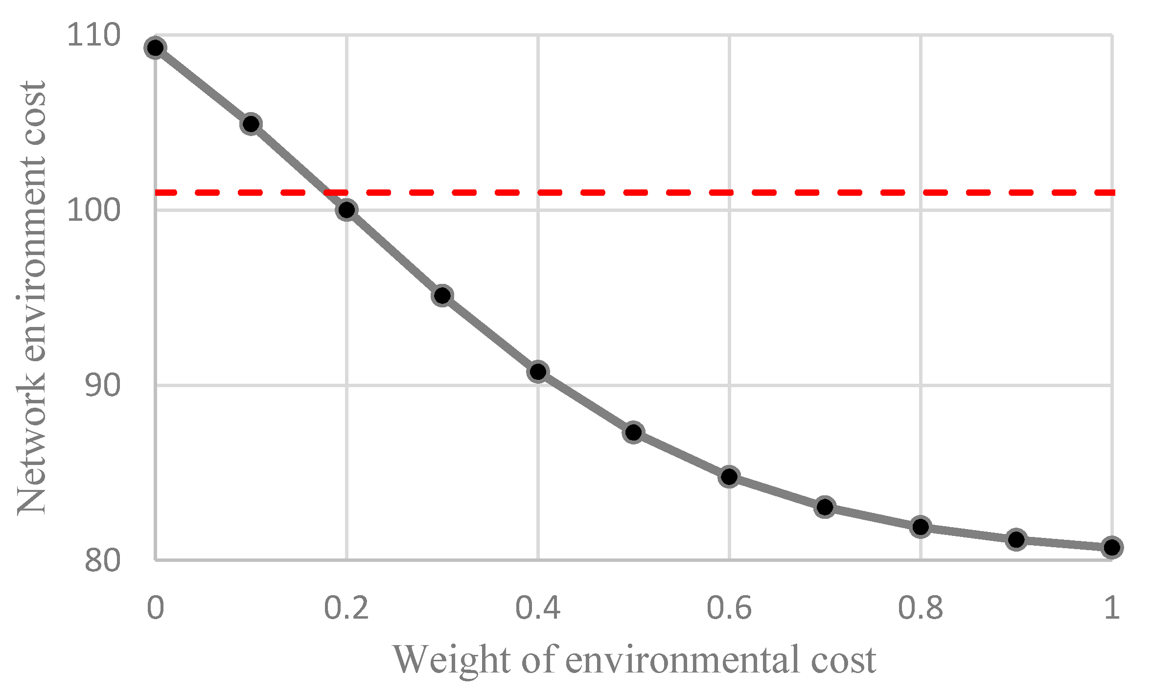
We considered incorporating the information of environmental cost into ATIS, and continually increased the weight of environmental cost to reduce the environmental cost and avoid such aforementioned traffic paradoxes. To test the scheme, we fixed $\eta =1$ and varied the weight of environmental cost $\gamma$ from 0 to 1, where the result of the actual environmental cost of the network is shown in Figure 4. Note that the initial point is the worst case where $\eta =1$ and $\gamma =0$, and the red dotted line is the reference line representing the condition where $\eta =0$ (there are no ATIS equipped drivers) and $\gamma =0$. It is clear that increasing the weight of environmental cost in ATS can effectively reduce the actual environmental cost of the transportation network. However, we should increase it to about 0.2 to have less actual environmental costs than the reference condition. Specifically, the network environmental cost decreases 26.76% when the weight of environmental cost increases from 0 to 1.

This example further indicates the motivation of our research and illustrates why we consider such a scheme incorporating the information into ATIS will ease the environmental problems caused by traffic. Note that this phenomenon appears because the shortest travel time route is not equivalent to the route with the minimum environmental cost between O–D pairs. This also explains the motivation of some researches to find the so-called green or environment-friendly routes [15,16,17,18,19]. Although this two-link network is very clear to illustrate our ideas, it is too small. We will further test our model and algorithm in larger networks in the next Section 4.2 and Section 4.3.

4.2. Nguyen-Dupuis Network

The proposed scheme and network equilibrium model are applied to the Nguyen-Dupuis network with 13 nodes and 19 links, where its topology is presented in Figure 5. Four O–D pairs are considered in this network, which are shown on the left side of Figure 5. The number of alternative routes between these O–D pairs are 8, 6, 5, and 6, respectively. The travel demands for each O–D pair are given as $q_{12}=400$, $q_{13}=800$, $q_{41}=600$, and $q_{43}=200$. The values of $t_a^0$, $C_a$, and $l_a$ are listed on the right side of Figure 5.

Depending on the research of interest, the transportation network problem can be analyzed at different levels, i.e., link level, route level, O–D level and network level, and all these levels deserve further studies. For example, at the link level problem, some researches focus on link emission restriction, and this problem is equivalent to the capacitated traffic assignment problems (CTAPs) [35]. However, traffic managers care more about the macroscopic level of problems and pay more attention to the O–D level and network level performance. To unify the order of magnitude, we use the unit environmental cost (UEC) of the O–D pair and transportation network as the indicators to analyze the problems at O–D level and network-level. Here, the UEC is defined as the value of total environmental cost dividing the total traffic demands of O–D pairs or the transportation network.

Firstly, we fix three levels of the environmental cost weights and vary the ATIS market penetration to analyze the effect of ATIS market penetration. The results of O–D level and network level are shown in Figure 6 and Figure 7, respectively. When we set a low environmental cost weight, i.e., $\gamma =0.3$, the UEC of some O–D pairs do not decrease but increase with the increase of ATIS market penetration, and the UEC of the network increases about 0.8%. This means the traffic paradox mentioned in Section 3.1 still exists. However, if we set the environmental cost weight at a high level, i.e., $\gamma =0.8$, the UEC of all O–D pairs and the whole network decrease. Specifically, the UEC decreases 5.2% when ATIS market penetration increases from 0 to 1.

We also considered the effect of environmental cost weight on UEC, when the ATIS market penetration is fixed. Three levels of ATIS market penetration were adopted, and the environmental cost weight was varied from 0 to 1. The results of O–D level and network level are shown in Figure 8 and Figure 9, respectively. It was obvious that the increase of environmental cost weights were always effective in reducing the UEC, no matter at low or high levels of ATIS market penetration. The higher the ATIS market penetration was, the more effective the scheme was. If the ATIS market penetration was 0.8, the UEC of O–D 4 decreased about 12.7%, when the environmental cost weight increased from 0 to 1. Furthermore, the UEC of the whole network greatly decreased by about 7.5%.

It is possible that someone would think the decrease rate of UEC at network level is not so significant, because it is not more than 10%. However, note that the traffic demands on the network are large. For example, the number of Chinese motor vehicles was more than two hundred million at the end of 2017. Even a small decrease rate multiplied by such a large base could reduce environmental costs significantly. Moreover, the travel behaviors occur every day, so the reduction is sustainably effective.

4.3. Sioux-Falls Network

Transportation problems are always considered as a complex problem, especially the traffic assignment problems. One of the main reasons is that the actual transportation network consists large numbers of links and O–D pairs, and the number of variables and parameters in models increases geometrically, which makes the problem more complex to be solved. Therefore, we also considered the computational efficiency of the proposed algorithm, which decides the application of models.

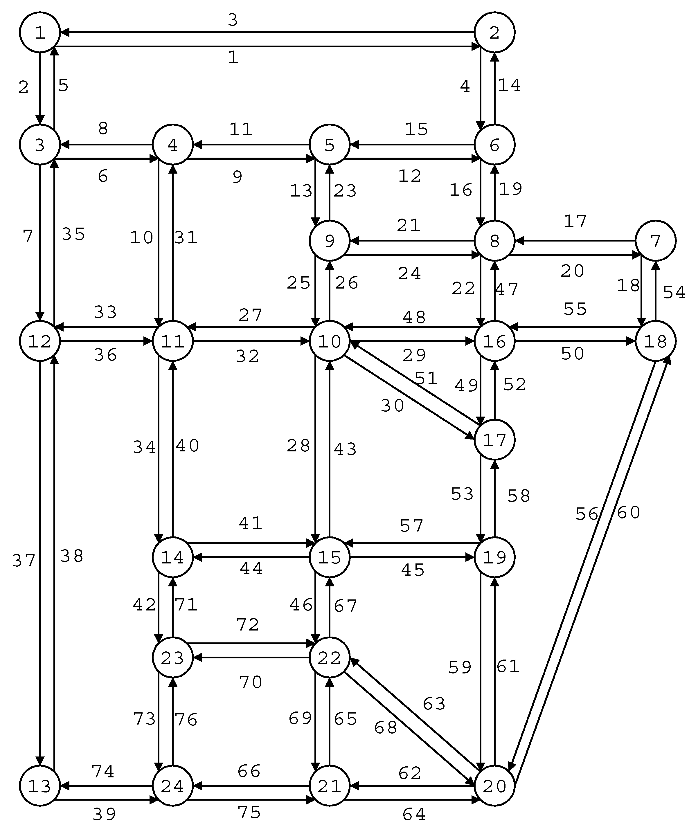
The well-known Sioux Falls network is used to illustrate the computational efficiency and applicability of the proposed algorithm [36]. As shown in Figure 10, the network consists of 24 nodes, 76 links, and 550 O–D pairs. A behaviorally generated working route set, which has 3441 routes, from Bekhor was used [37]. Correspondingly, the notation ${\delta }_{w,k,a}$ denotes 3441 × 76 parameters, and the scale of the model was quite large. The length of each link was the same as the input data proposed by Reference [36]. The values of link free travel time, link capacity and O–D traffic demand followed those proposed by Reference [38].

The iterative processes of the accuracy and network level environmental cost is shown in Figure 11. Both can rapidly converge to the stable values and the accuracy reach $1\times {10}^{-5}$ only uses 95 iterations, which only cost about 0.19 s CPU time. With the increase of iteration number, network level environmental cost continuously decreased to the stable value of 1,390,740, which meant the descent direction in step 3 of the proposed algorithm was effective and right. No “zig-zag” was observed during the whole convergence process. It meant the set of step size was appropriate. Based on the analysis above, our proposed algorithm is obviously highly efficient and applicable to a large-scale network.

5. Conclusions

This paper proposed a new scheme which incorporates the information of environmental cost into the ATIS to guide drivers route choice. With this consideration, ATIS can provide drivers with more environment-friendly routes and help reduce the environmental cost of the transportation network. Based on the basic idea, we use the theory of network equilibrium to analyze the effect of this new scheme. The mixed SUE model was proposed to describe the interactive route choice behaviors between ATIS equipped and unequipped drivers. We also formulated the mixed SUE model as an FPP. Then a logit-based MSA algorithm was proposed to solve this model.

Three numerical examples were provided to illustrate the essential ideas of the proposed model and test the capability of the solution algorithm. The results of the examples confirmed the effectiveness of our proposed management scheme. Firstly, in a simple two-link network, one traffic paradox phenomenon was analyzed, which indicated that providing better travel time information to more travelers may lead to higher environmental costs of the transportation network. Moreover, our proposed scheme can be used to avoid such a traffic paradox. This finding further illustrates the motivation of our research. Then the validity of our schemes were further verified in the Nguyen-Dupuis network. We found that the increase of ATIS market penetration may lead to the increase of network environmental cost with a low environmental cost weight in ATIS. However, regardless of low or high ATIS market penetration, the increase of the environmental cost weight can decrease network environmental cost. Finally, we tested the computational efficiency of the proposed algorithm in a large scale of Sioux-Falls network. The result showed it only takes 0.19 s CPU time to converge to high accuracy. Therefore, our proposed model and algorithm can be well applied to a large-scale transportation network.

As we know, research and development of advanced eco vehicles requires a lot of manpower and material resources, and it cannot be widely popularized in a short time due to its high cost and technical problems. For example, electric vehicles are generally more expensive than gasoline vehicles, whilst the driving range of electric vehicles is shorter. Whilst effective management policy can achieve benefits in the short term, the results of our research show policy makers that using ATIS to guide travelers for green route choices is an effective scheme to reduce the environmental cost of the transportation network. Furthermore, no new technology problem should be solved in this scheme, so it is easy to be realized in the short term. However, developing environmentally friendly vehicles and implementing the scheme of guiding green routes have no conflicts, they can be conducted at the same time.

The present paper still has some limitations. Given we employed the theory of transportation network equilibrium, more realistic and practical assumptions should be considered into the model in the future. For example, bounded rationality is an emerging research subject due to its power in more realistic traffic behavior. Moreover, we tend to combine the traffic modal split and route choice behavior into one model. If people can choose both more environment-friendly traffic modes and routes, this can better reduce the environmental cost of the transportation network.

References

- Xu, X.; Chen, A.; Yang, C. A review of sustainable network design for road networks. KSCE J. Civ. Eng. 2016, 20, 1084–1098. [Google Scholar] [CrossRef]
- Wang, X.; Shao, C.; Yin, C.; Zhuge, C. Exploring the Influence of Built Environment on Car Ownership and Use with a Spatial Multilevel Model: A Case Study of Changchun, China. Int. J. Environ. Res. Public Heal. 2018, 15, 1868. [Google Scholar] [CrossRef] [PubMed]
- Alves, C.A.; Gomes, J.; Nunes, T.; Duarte, M.; Calvo, A.; Custódio, D.; Pio, C.; Karanasiou, A.; Querol, X. Size-segregated particulate matter and gaseous emissions from motor vehicles in a road tunnel. Atmos. Res. 2015, 153, 134–144. [Google Scholar] [CrossRef]
- Worton, D.R.; Isaacman, G.; Gentner, D.R. Lubricating oil dominates primary organic aerosol emissions from motor vehicles. Environ. Sci. Technol. 2014, 48, 3698–3706. [Google Scholar] [CrossRef] [PubMed]
- Gentner, D.R.; Jathar, S.H.; Gordon, T.D.; Bahreini, R.; Day, D.A.; El Haddad, I.; Hayes, P.L.; Pieber, S.M.; Platt, S.M.; Gouw, J.D. Review of urban secondary organic aerosol formation from gasoline and diesel motor vehicle emissions. Environ. Sci. Technol. 2017, 51, 1074–1093. [Google Scholar] [CrossRef] [PubMed]
- Ajanovic, A.; Dahl, C.; Schipper, L. Modelling transport (energy) demand and policies—An introduction. Energy Policy 2012, 41, 3–16. [Google Scholar]
- Alshehry, A.S.; Belloumi, M. Study of the environmental Kuznets curve for transport carbon dioxide emissions in Saudi Arabia. Renew. Sustain. Energy Rev. 2017, 75, 1339–1347. [Google Scholar] [CrossRef]
- Centobelli, P.; Cerchione, R.; Esposito, E. Environmental sustainability and energy-efficient supply chain management: A review of research trends and proposed guidelines. Energies 2018, 11, 275. [Google Scholar] [CrossRef]
- Shindell, D.; Faluvegi, G.; Walsh, M.; Anenberg, S.C.; Van Dingenen, R.; Muller, N.Z.; Austin, J.; Koch, D.; Milly, G. Climate, health, agricultural and economic impacts of tighter vehicle-emission standards. Nat. Clim. Chang. 2011, 1, 59. [Google Scholar] [CrossRef]
- An, F.; Earley, R.; Green-Weiskel, L. Global Overview on Fuel Efficiency and Motor Vehicle Emission Standards: Policy Options and Perspectives for International Cooperation; United Nations Background Paper; Commission on Sustainable Development: New York, NY, USA, 2011; Volume 3. [Google Scholar]
- An, F.; Sauer, A. Comparison of Passenger Vehicle Fuel Economy and Greenhouse Gas Emission Standards around the World; Pew Center on Global Climate Change: Arlington, VA, USA, 2004; Volume 25. [Google Scholar]
- Zheng, B.; Zhang, Q.; Borken-Kleefeld, J.; Huo, H.; Guan, D.; Klimont, Z.; Peters, G.; He, K. How will greenhouse gas emissions from motor vehicles be constrained in China around 2030? Appl. Energy 2015, 156, 230–240. [Google Scholar] [CrossRef] [Green Version]
- Kitthamkesorn, S.; Chen, A.; Xu, X.; Ryu, S. Modeling mode and route similarities in network equilibrium problem with go-green modes. Netw. Spat. Econ. 2016, 16, 33–60. [Google Scholar] [CrossRef]
- Lin, Z.; Greene, D.L. Promoting the market for plug-in hybrid and battery electric vehicles: Role of recharge availability. Transp. Res. Rec. 2011, 2252, 49–56. [Google Scholar] [CrossRef]
- He, F.; Yin, Y.; Lawphongpanich, S. Network Equilibrium Models with Battery Electric Vehicles. Transp. Res. Part B Methodol. 2014, 67, 306–319. [Google Scholar] [CrossRef]
- Bektaş, T.; Laporte, G. The pollution-routing problem. Transp. Res. Part B Methodol. 2011, 45, 1232–1250. [Google Scholar] [CrossRef]
- Demir, E.; Bektaş, T.; Laporte, G. The bi-objective pollution-routing problem. Eur. J. Oper. Res. 2014, 232, 464–478. [Google Scholar] [CrossRef]
- Nagurney, A. Congested urban transportation networks and emission paradoxes. Transp. Res. Part D Transp. Environ. 2000, 5, 145–151. [Google Scholar] [CrossRef]
- Li, Q.; Nie, Y.M.; Vallamsundar, S.; Lin, J.; Homem-de-Mello, T. Finding efficient and environmentally friendly paths for risk-averse freight carriers. Netw. Spat. Econ. 2016, 16, 255–275. [Google Scholar] [CrossRef]
- Li, W.; Yang, L.; Wang, L.; Zhou, X.; Liu, R.; Gao, Z. Eco-reliable path finding in time-variant and stochastic networks. Energy 2017, 121, 372–387. [Google Scholar] [CrossRef] [Green Version]
- Levinson, D. The value of advanced traveler information systems for route choice. Transp. Res. Part C Emerg. Technol. 2003, 11, 75–87. [Google Scholar] [CrossRef] [Green Version]
- Cheng, L.; Lou, X.; Zhou, J.; Ma, J. A mixed stochastic user equilibrium model considering influence of advanced traveller information systems in degradable transport network. J. Cent. South Univ. 2018, 25, 1182–1194. [Google Scholar] [CrossRef]
- Jafari, E.; Boyles, S.D. Multicriteria stochastic shortest path problem for electric vehicles. Netw. Spat. Econ. 2017, 17, 1043–1070. [Google Scholar] [CrossRef]
- Li, D.; Miwa, T.; Morikawa, T.; Liu, P. Incorporating observed and unobserved heterogeneity in route choice analysis with sampled choice sets. Transp. Res. Part C Emerg. Technol. 2016, 67, 31–46. [Google Scholar] [CrossRef]
- Benedek, C.M.; Rilett, L.R. Equitable traffic assignment with environmental cost functions. J. Transp. Eng. 1998, 124, 16–22. [Google Scholar] [CrossRef]
- Ma, J.; Cheng, L.; Li, D.; Tu, Q. Stochastic Electric Vehicle Network Considering Environmental Costs. Sustainability 2018, 10, 2888. [Google Scholar] [CrossRef]
- Ma, J.; Li, D.; Cheng, L.; Lou, X.; Sun, C.; Tang, W. Link restriction: Methods of testing and avoiding braess paradox in networks considering traffic demands. J. Transp. Eng. Part A Systain. 2018, 144. [Google Scholar] [CrossRef]
- Guo, X.; Yang, H.; Liu, T.L. Bounding the inefficiency of logit-based stochastic user equilibrium. Eur. J. Oper. Res. 2010, 201, 463–469. [Google Scholar] [CrossRef] [Green Version]
- Dell’Orco, M.; Marinelli, M. Modeling the dynamic effect of information on drivers’ choice behavior in the context of an Advanced Traveler Information System. Transp. Res. Part C Emerg. Technol. 2017, 85, 168–183. [Google Scholar] [CrossRef]
- Li, D.; Miwa, T.; Morikawa, T. Considering en-route choices in utility-based route choice modelling. Netw. Spat. Econ. 2014, 14, 581–604. [Google Scholar] [CrossRef]
- Sheffi, Y. Urban Transportation Networks; Prentice-Hall: Englewood Cliffs, NJ, USA, 1985. [Google Scholar]
- Nagurney, A.; Dong, J. A multiclass, multicriteria traffic network equilibrium model with elastic demand. Transp. Res. Part B Methodol. 2002, 36, 445–469. [Google Scholar] [CrossRef]
- Huang, H.J.; Li, Z.C. A multiclass, multicriteria logit-based traffic equilibrium assignment model under ATIS. Eur. J. Oper. Res. 2007, 176, 1464–1477. [Google Scholar] [CrossRef]
- Murchland, J.D. Braess’s paradox of traffic flow. Transp. Res. 1970, 4, 391–394. [Google Scholar] [CrossRef]
- Nie, Y.; Zhang, H.M.; Lee, D.H. Models and algorithms for the traffic assignment problem with link capacity constraints. Transp. Res. Part B Methodol. 2004, 38, 285–312. [Google Scholar] [CrossRef]
- Leblanc, L.J. An algorithm for the discrete network design problem. Transp. Sci. 1975, 9, 183–199. [Google Scholar] [CrossRef]
- Bekhor, S.; Toledo, T.; Prashker, J.N. Effects of choice set size and route choice models on path-based traffic assignment. Transportmetrica 2008, 4, 117–133. [Google Scholar] [CrossRef]
- Sun, C.; Cheng, L.; Zhu, S.; Han, F.; Chu, Z. Multi-criteria user equilibrium model considering travel time, travel time reliability and distance. Transp. Res. Part D Transp. Environ. 2017. [Google Scholar] [CrossRef]
Figure 1.
Flowchart for the procedure of the algorithm.
Figure 2.
Two-link network for illustration.
Figure 3.
The effect of the advanced traveler information system (ATIS) market penetration on network environmental cost.
Figure 4.
The effect of environmental cost weight on network environmental cost.
Figure 5.
Topology and link parameters of Nguyen-Dupuis network.
Figure 6.
The effect of ATIS market penetration on origin–destination (O–D) level environmental cost.
Figure 7.
The effect of ATIS market penetration on network level environmental cost with different environmental cost weights.
Figure 8.
The effect of environmental cost weight on O–D level environmental cost.
Figure 9.
The effect of environmental cost weight on network level environmental cost with different ATIS market penetrations.