Probabilistic Forecasting of Nitrogen Dioxide Concentrations at an Urban Road Intersection

Abstract

The concentration of nitrogen dioxide in the air along a major route in a large city is affected by very many factors, which are also interdependent. As an alternative to complicated deterministic models based on these complex processes, in this study a probabilistic model for predicting NO₂ concentrations is proposed, using a simple accounting cluster-based method for determining probability distributions for tabulated values of ambient factors. Using the example of hourly values of NO₂ concentration and data on wind speed and traffic flow for the main intersection in Wrocław (Poland), a model is constructed to predict the frequency of occurrence of concentrations in the form of a probability distribution, for given values of the input variables. The model was successfully verified on data for the first six months of 2018. A mean continuous rank probability score (CRPS) of 9.15 μg/m³ was obtained. In spite of the greater impact of traffic volume on urban NO₂ concentrations, as measured by Pearson’s correlation coefficient, for instance, the model indicates that wind speed is also a very important factor—wind being the principal mechanism causing the evacuation of pollutants. This underlines the importance of sustainable city planning with regard to ensuring suitable conditions for the passage of air.

1. Introduction

With the increase in levels of anthropogenic air pollution, there is growing interest among scientists in modelling the relationship between pollutant concentrations and various ambient factors. Methods of forecasting pollution levels on various timescales are being simultaneously developed. Literature reports indicate that atmospheric concentrations of pollutants are affected fundamentally both by the pollutant load (originating from various sources) and by meteorological conditions in the area studied. The main source of emissions of nitrogen oxides is waste gases, which come mainly from high-temperature combustion in vehicle engines, as well as from the combustion of fuels in energy production. In transport, the largest emitters of NO₂ are diesel engines. Known deterministic models describing relationships between pollutant concentrations in the air and meteorological and temporal conditions and traffic flow may be divided into two groups, based on localization in time: Current (point-based) and backward (interval-based). Interval-based models require and use data from a certain preceding period of time (t − 1, t − 2, t − 24, t − 48) to determine the predicted value at time t. This is quite a well-understood approach, with over 90% prediction effectiveness e.g., [1,2,3,4]. Point-based models, on the other hand, serve to determine the pollutant concentration value based on data only from the time point t. There is still much to be done with regard to point-based models, because their quality of fit needs improvement, and their predictive capabilities are burdened with a large error. Among point-based models, one may identify several principal methods of mathematical modelling. Still popular are regression models, which have evolved significantly due to the development of computational techniques [5,6,7,8]. More computationally advanced are models based on machine learning. Models that have been applied include artificial neural networks [9,10], which may also be combined with a multiple regression model [11]. There is an increasing number of reports on the use of random tree methods to model pollutant concentrations. These include both single random trees [12] and more complex structures based on them: Random forest (RF) [13,14] and boosted regression trees (BRT) [15]. Singh et al. [12] compared the effectiveness of methods based on random trees and on support vector machines (SVMs) in modelling atmospheric pollutant concentrations, and found that the random trees outperformed SVMs. Comparisons of the RF and BRT methods have not yet determined conclusively the advantage of either modelling method over the other. Singh et al. [12] do not indicate that either method is superior. Kamińska [16] states that for the prediction of typical values better results are obtained by the BRT method, while for the prediction of higher values the RF method gives better results.

Deterministic models, particularly those that do not refer to the values of variables at preceding time points (point-based models), are subject to large errors, and the main problem with their application is their poor fit to data. Larkin et al. [17] based on worldwide data from 5220 air monitors from 58 countries on all over the world developed the Land Use Regression model based on 10 land use predictors with R² = 0.52. Sayegh et al. [15] for the input data, including meteorological conditions, temporal data and traffic flow obtained R² from 0.49 to 0.54 for different measurement points. Kamińska [18] performed a modification of an RF model, which improved the quality of fit to R² = 0.82, although there were difficulties in making predictions. This fact results from the high variability of concentration values and the significant number of factors on which those values depend. Attempts to forecast a precise numerical value led to very large errors. An alternative to deterministic models is probabilistic models, which may be used to forecast concentrations or the exceeding of threshold values with given probability [19,20].

Probabilistic models serve to generate a forecast in the form of probability values or a probability distribution for the occurrence of an event, given the existence of specified conditions. In the field of air pollution, such models give the probability (or a probability distribution) of a pollutant concentration subject to specified ambient conditions (values of explanatory variables). Probabilistic models perform particularly well in forecasting the values of variables in the case of heavily skewed data, when the accuracy of deterministic models is greatly reduced. The literature describes three main modelling techniques for probabilistic forecasting of air pollution concentration: Quantile regression, modelling based on weather forecasting, and ensemble statistical post-processing. Probabilistic forecasting with quantile regression is based on the conditional sample mean, but instead of the mean the median is estimated. In the case of forecasting of extreme values or concentration peaks, the median is replaced by any quantile [19,20]. Probabilistic models based on weather forecasting are complex models consisting of several modules, including a module for forecasting meteorological conditions, a module for forecasting pollutant emissions, and a final module for forecasting the pollutant concentration. The main drawback of this method is the need to predict the input conditions for the pollutant concentration model, which entails a high degree of uncertainty. Weather forecasts may be obtained using the model of [21] or taken from a reliable source [22]. Such models enable forecasting for arbitrarily large areas. Another difficulty in the application of forecasts of this type is the complex construction of the model and its interdisciplinary nature. Another type of probabilistic forecasting makes use of an ensemble statistical post-processor (ESP). An example is the work of Garner and Thompson [23], where an ESP is constructed using a moving-block bootstrap, regression trees and extreme-value theory for the forecasting of concentrations of ozone.

In this study a probabilistic model is proposed that enables the forecasting of atmospheric pollutant concentrations, and which may be easily implemented at any location along a transport route. A basic condition and limitation required for the model to be effective is that traffic flow and air quality measuring points should be situated close to one another. It was reported by Padró-Martínez et al. [24] and Beckerman et al. [25] that the highest NO₂ concentrations are found within 50 m of the road, and then fall off with increasing distance. A second factor determining the effectiveness of the model is the appropriate selection of explanatory variables (predictors). Most studies use sets of variables reflecting traffic and meteorological conditions [15,26,27]. There also exist studies based only on meteorological data [28] or only on traffic data [29]. More precise analysis of the effect of particular explanatory variables is enabled by such methods as random trees. The methodology for identifying tree divisions described by Breiman [30] allows the importance of predictors to be determined on a scale of 0–100. Using this methodology, Kamińska [13] established that the most significant variables affecting NO₂ concentration were traffic flow and wind speed. Anzarte [19], who studied the importance of variables according to a concept based on a direct measure of the impact of each feature on the accuracy of the model [31], identified as the most important factors (apart from variables referring to preceding time points) the temperature and wind speed. One could find papers with different, temporal variables, such as: Month, hour of the day [14], weekday, weekend or holiday [13,32], but their impact on the variability of the pollution concentration is slight.

The idea of the present approach is to partition the entire dataset into clusters by a matrix method, with respect to the values of the explanatory variables that modelling shows to be the most important. For each cluster, a probabilistic analysis is performed, and a forecast is obtained. This takes the form of a probability distribution for NO₂ concentrations or the probability of the exceeding of a set threshold of pollutant concentration (e.g., limit, warning, alarm levels), for given values of the explanatory variables.

Determination of the probability of occurrence of warning and alarm levels of NO₂ subject to given values of traffic flow can help traffic managers to take decisions efficiently, by selecting the most adequate traffic management strategy [33,34,35,36]. In Wrocław, rational spatial planning encouraging the maintenance of favorable environmental conditions is not yet established practice [37]. The adverse impact of new buildings may be observed not only within the city, but also in new suburban developments [38]. Most new buildings in Wrocław do not form compact groups that might ensure free space for the passage of air. Hope for a change to current practices is provided by the adopted Polish National Strategy for Adaptation to Climate Change in the Perspective to 2030, which requires cities with more than 100,000 inhabitants to prepare their own plans for adaptation to climate change [39]. Although the main emphasis in this strategy is on rainwater management, the document creates the possibility of integrated and systematic management of various environmental components, including air quality. A systematic approach to the sustainable management of city development, making use of wind conditions, is effectively implemented in Wrocław and its surroundings with the use of spatial analyses and decision support systems for urban planning [40]. The results of the present study may therefore prove useful in efforts to improve air quality in Wrocław.

The model makes it possible, in a simple manner, to forecast probability distributions for pollution levels depending on the values of the input parameters. This makes it easy to determine what changes in air quality can be expected to result from a given reduction in the number of vehicles driving into the city center. This will enable estimation of the benefits resulting from, for example, the introduction of a charge for vehicles entering the central zone.

2. Materials and Methods

2.1. Methodology

As was mentioned at the outset, precise numerical forecasting of atmospheric pollutant concentrations, without taking past values into account of past values, is subject to very large errors. An alternative to deterministic methods is a probabilistic approach. Pollutant concentrations are subject to a high degree of variation. In the present approach, the dataset is partitioned into clusters based on ranges of the values of the independent variables. Assuming that two independent variables are being considered, the clusters will be described by a matrix system. More generally, the system will have a number of dimensions equal to the number of independent variables. Thus, the entire dataset is represented by the matrix $D=\left[Y,X_1,X_2,\dots ,X_n\right]$, where Y is a vector of values of the dependent variable, and $X_k$ $\left(k=1,\dots ,K\right)$ are vectors of explanatory variables (predictors). This set is divided into subsets (clusters) according to the values of the explanatory variables. In view of limitations resulting from the methodology of analysis of the conformity of a random variable to a theoretical distribution, the number of explanatory variables must be small enough to ensure that each cluster contains a sufficient number of cases. As mentioned above, in the problem under consideration there are two highly significant explanatory variables, and our further considerations will therefore concern this case.

The values of the variables $X_1$, $X_2$ are partitioned into $n_1$ and $n_2$ intervals respectively. This division leads to $n_1·n_2$ subsets (clusters) of data represented by matrices $D_{i,j}=\left[Y_{ij},X_{1ij},X_{2ij}\right]$, where $i=1,2,\dots ,n_1$, $j=1,2,\dots ,n_2$. For each cluster independently, a probability distribution is determined for the variable $Y_{i,j}$. Knowledge of the probability distribution of pollutant concentrations within a bounded space of ambient conditions enables one to determine the probability that a given concentration threshold $y_0$ will be exceeded when such conditions exist.

$$P_{a_{1i}{a}_{2j}}\left(y_0\right)=P(Y>y_0|a_{1i}<X_1\le a_{1i+1} \wedge a_{2j}<X_2\le a_{2j+1}).$$

(1)

Here $a_{1i},a_{2j}$ are the boundary values of the partition of $X_1, X_2$ respectively.

Knowing a theoretical probability distribution that conforms to the empirical distribution of the variable $Y_{i,j}$, and thus also its distribution function, one may also use this method to calculate a concentration value that will be exceeded with given probability, assuming a defined set of conditions.

The effectiveness of the method may be impaired if the data subsets are of insufficient size. It may then be difficult to fit the data to a theoretical distribution and to obtain statistically significant conformity. The partitioning of values of the explanatory variables must therefore be performed in such a way as to ensure a minimum number of instances of the variable $Y_{ij}$ to enable the procedure of fitting a theoretical probability distribution to be carried out. It is recommended that the size of clusters should be such that, when classes are formed in the process of determining the value of a test statistic, the number of cases in each class is at least 5 [41]. In practice, a minimum number of 30 cases is used. The described procedure may be used for any atmospheric pollutant, once a set of predictors has been identified. It is important that the air quality measuring station should be located not more than 50 m from the road being the source of the pollution.

In this study, the above procedure was applied to the analysis and forecasting of values of nitrogen dioxide concentrations in the air along a major transport route, using the example of a selected road intersection in the city of Wrocław (Poland).

2.2. Data Sources

Wrocław is located in the southwestern part of Poland (Europe). The intersection of the streets Hallera and Powstańców Śląskich is subject to traffic flow monitoring, and an air quality measuring station is located in its vicinity. In view of the significant dependence of atmospheric pollutant concentrations on the distance from the road, computations were carried out on the basis of data obtained from this intersection.

Based on values of Pearson’s correlation coefficient (

Table 1. Pearson correlation coefficient for NO₂ concentration and predictors (all coefficients statistically significant for $\alpha =0.05$.

Predictor	Correlation Coefficient
Traffic flow	0.494723
Wind speed [m/s]	−0.249011
Relative humidity [%]	−0.189845
Air temperature	0.141084
Air pressure [hPa]	0.045151
Month (1–12)	−0.030458
Day of the week (1–7)	−0.013921

), and the results of studies which included analysis of the impact (importance) of different variables on NO₂ concentrations, carried out at the same intersection for the years 2015–2016 [13] and 2015–2017 [18], it was concluded that the greatest influence on concentrations comes from two variables: Traffic flow and wind speed. These were selected as the independent variables to be used for further analysis.

In the dataset covering a total of 26,081 h of measurements, a small number of missing or erroneous readings were present, due to temporary faults of the automatic measuring systems. Cases for which the value of at least one variable was absent or the values were incorrect (traffic flow exceeding the capacity of the intersection) were excluded from the analysis. The number of cases thus omitted was 310, equal to 1.2% of the original number of cases.

2.2.1. NO₂ Concentrations

Measurements of nitrogen dioxide concentration were made at five points, but only one near the largest crossroads in central Wrocław: The intersection of the streets Hallera and Powstańców Śląskich (Figure 1). The data cover the full years 2015–2017 and were collected by the Provincial Environment Protection Inspectorate. Basic statistical values relating to NO₂ concentrations are given in

Table 2. Descriptive statistic for all variables.

Variable	Mean	Median	Min.	Max	Stand. Dev.
NO2 concentration [μg/m3]	50.4	49.4	1.7	231.6	23.2
Traffic flow $\left[\mathrm{veh}\right]$	2773	3179	44	5712	1795
Wind speed $\left[\mathrm{m}·{\mathrm{s}}^{-1}\right]$	3.1	3.0	0	19	2.0

.

The limit annual average value of NO₂ is 40 μg/m³ and was exceeded at that station in each of the years 2015–2017, reaching 53.8, 49.2 and 48.1 μg/m³. The median of NO₂ concentration (49.4 μg/m³) is lower than the mean (50.4 μg/m³) which indicates the right-sided asymmetry (shown in Figure 2). The permissible hourly atmospheric concentration of NO₂ in Poland is 200 μg/m³, and this value must not be exceeded more than 18 times in a year. The alarm level of atmospheric NO₂ is 400 μg/m³ maintained for at least three consecutive hours [Regulation of the Minister of Environment of 14 August 2012 on levels of certain substances in the air]. In the analysed period, the permissible hourly level was exceeded on three occasions in 2015 (30.08, 01.09 and 04.11—two consecutive hours), but the alarm hourly level was not attained. A frequency histogram for nitrogen dioxide concentrations is presented in Figure 2. For the complete dataset, parameters were determined for the following asymmetric continuous theoretical distributions: Weibull, Johnson, generalised extreme value (GEV) and log-normal. The values of the ${\chi }^2$ and Anderson–Darling statistics were high, and the corresponding p-values did not differ from zero (with an accuracy to five decimal places). Values of the less restrictive Kolmogorov–Smirnov (K-S) statistic gave p-values of 0.025, 0.029, 0.033 and 0.085 for the respective distributions. However, in the light of the results of the other tests, this does not enable confirmation of the conformity of the empirical distribution to any of the analysed theoretical distributions.

2.2.2. Traffic Flow

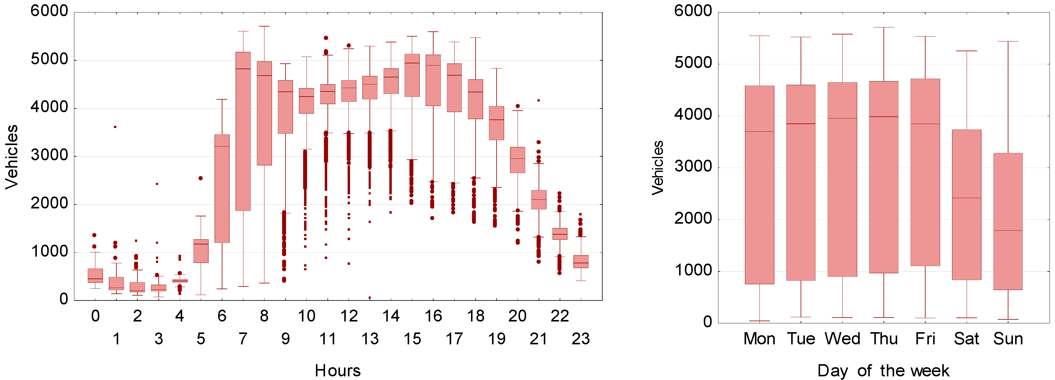
The traffic data are provided by the Traffic and Public Transport Management Department of the Roads and City Maintenance Board in Wrocław. The Department operates 921 video cameras distributed widely over the area of the city. One of the pieces of information obtained is the number of vehicles passing through the measurement plane on a given traffic lane or lanes. A network of sensors is set up to monitor vehicular traffic at the main intersections of the city road network. A total of 68 intersections are subject to traffic measurement. However, only in one case is a monitored intersection located in the immediate vicinity of an air quality measuring station: At the intersection of Hallera and Powstańców Śląskich. Traffic flow data indicate the total number of vehicles driving onto the intersection from all directions and traffic lanes. The daily and weekly variation in traffic flow values are shown in Figure 3.

The daily variation in traffic volume is bimodal, with peak periods in the morning between 7:00 and 8:00 and in the afternoon between 15:00 and 17:00, although the variation during the morning peak is significantly greater than during the afternoon peak. During night time the traffic flow is significantly lower. The traffic volumes on working days are similar, but there is a clear reduction at weekends.

2.2.3. Wind Speed

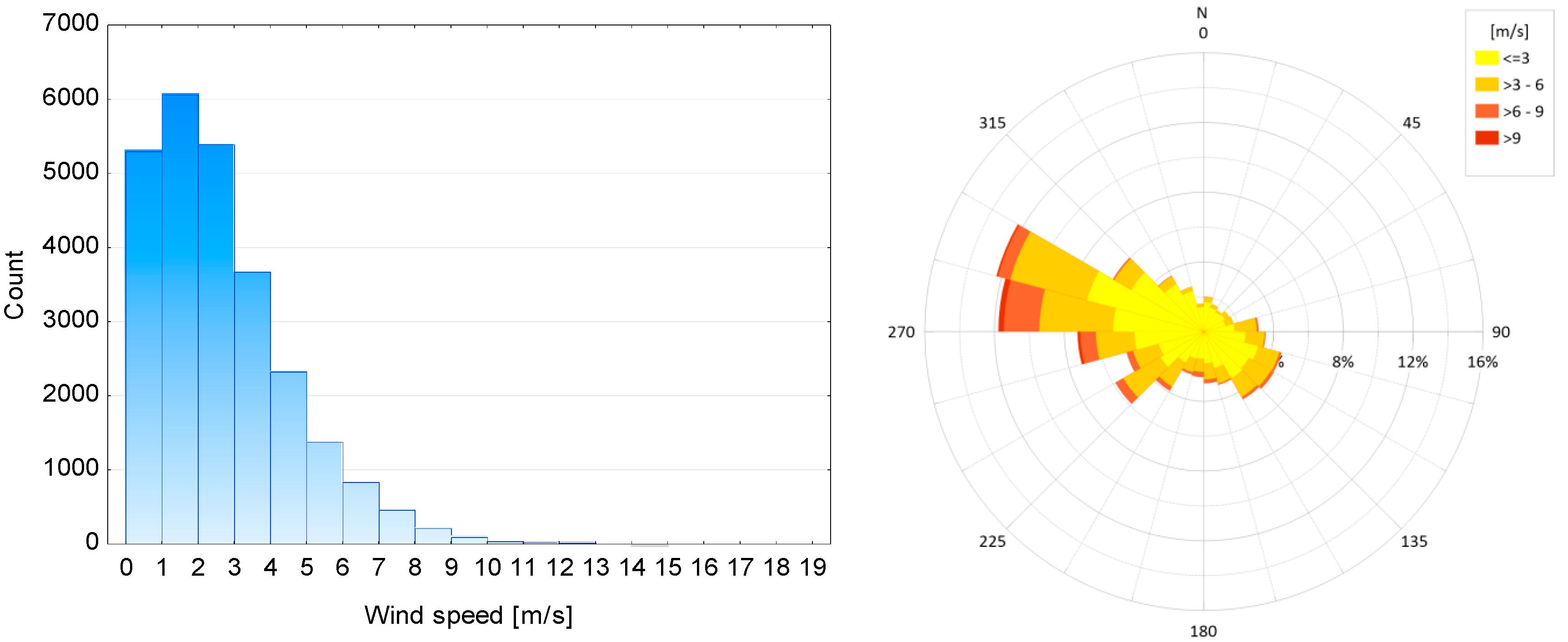
Meteorological data are provided by a measuring station of the Institute of Meteorology and Water Management in Wrocław, at Strachowice airport, located at a straight-line distance of 9.6 km from the analysed intersection. Hourly values are taken from automatic measuring equipment, and are computed as the means of instantaneous measurements taken in the course of an hour. For the reasons explained in Section 3, only wind speed values are considered in this analysis. In Wrocław, W and WNW winds are most prevalent, and their speeds are relatively low (Figure 4). The maximum observed wind speed was 19 m/s, the average being 3.1 m/s. There is strong right-sided asymmetry (Figure 4). Wind speeds exceeding 10 m/s were recorded only in 71 cases (hours) during the full three-year period.

3. Results and Discussion

3.1. Probability Distribution

As described in Section 2.2.1, the random variable representing values of NO₂ concentration is not found to conform to any of the theoretical distributions. Using the described methodology, the entire set of concentration values was divided into clusters according to the values of the independent variables (in this case, traffic flow and wind speed). The boundary values of these variables were determined a priori based on an analysis of their variability and the basic laws controlling the physics of pollutants in the air. Traffic flow values were partitioned at intervals of 1000 vehicles, mainly in order to ensure that the clusters were of adequate size. Wind speed values were partitioned at intervals of 2 m/s, on the grounds that:

• The first interval reflects conditions of very light wind or no wind, when the wind’s role in removing pollutants from the transport route is negligible, and the accumulation of pollutants favors the occurrence of chemical reactions in the air;
• Further intervals reflect conditions of increasing wind strength, which affects the rate of horizontal movement of pollutants;
• The final interval reflects strong winds (relative to normal local conditions), which, by causing movement of air through the city, affect the NO₂ concentration values.

The distance of the meteorological measuring station from the intersection (9.6 km) is not insignificant. The division into clusters defined above, based on wind speeds with a step size of 2 m/s, takes into account the possibility of modification of the value of this variable as a result of the distance.

Table 3. Numbers of cases in each cluster. Horizontally: Wind speed (m/s); vertically: Traffic flow (vehicles).

	$\left[0,2\right]$	$\left(2,4\right]$	$\left(4,6\right]$	$\left(6,8\right]$	$\left(8,+\mathit{\infty }\right)$
$\left(0, 1000\right]$	3991	2060	698	230	64
$\left(1000, 2000\right]$	1582	951	339	128	24
$\left(2000, 3000\right]$	985	748	315	118	33
$\left(3000, 4000\right]$	1550	1400	531	167	58
$\left(4000, 5000\right]$	2577	3125	1510	544	170
$\left(5000,+\infty \right)$	669	774	305	104	21

shows the number of cases in each cluster. Two clusters, marked in green, were too small to enable the conduct of the procedure to test conformity to a theoretical probability distribution.

For the values of NO₂ concentration corresponding to the cases contained in each cluster, corresponding parameters were computed for the following asymmetric continuous theoretical distributions: Weibull, Johnson, generalized extreme value (GEV) and log-normal. Next, for each theoretical distribution and each cluster, statistical tests of the fit of the theoretical and empirical distributions were performed: A ${\chi }^2$ test and a Kolmogorov–Smirnov (K-S) test. The Anderson–Darling test gave almost the same p-values as the ${\chi }^2$ tests, and therefore only the results of the latter are shown. The best fit (taking account of all clusters) was obtained for the log-normal distribution with density function given by (2):

$$f\left(x\right)=\frac{1}{x\sigma \sqrt{2\pi }}exp\left(\frac{-{\left(lnx-\mu \right)}^2}{2{\sigma }^2}\right).$$

(2)

Values of ${\chi }^2$ and Kolmogorov–Smirnov (K-S) statistics, together with computed p-values, are given in

Table 4. Values of test statistics, with p-values (in brackets).

Number of Vehicles	Statistical Test	$\left[0,2\right]$	$\left(2,4\right]$	$\left(4,6\right]$	$\left(6,8\right]$	$\left(8,+\mathit{\infty }\right)$
(0, 1000]	K-S	0.028 (0.0037)	0.020 (0.3988)	0.022 (0.8816)	0.052 (0.5376)	0.079 (0.7959)
	${\mathsf{\chi }}^2$	54.5 (0.0000)	10.4 (0.4975)	12.3 (0.5785)	7.2 (0.7098)	2.3 (0.8899)
(1000, 2000]	K-S	0.016 (0.7901)	0.035 (0.1987)	0.043 (0.5498)	0.144 (0.9576)
	${\chi }^2$	17.0 (0.4517)	16.5 (0.1222)	17.5 (0.2306)	10.8 (0.6318)
(2000, 3000]	K-S	0.029 (0.3598)	0.027 (0.6224)	0.043 (0.6044)	0.052 (0.8864)	0.101 (0.8548)
	${\chi }^2$	21.3 (0.0115)	16.8 (0.3339)	15.8 (0.2001)	8.5 (0.5826)	0.8 (0.8548)
(3000, 4000]	K-S	0.014 (0.9358)	0.023 (0.4696)	0.049 (0.1489)	0.058 (0.6070)	0.083 (0.7855)
	${\chi }^2$	11.3 (0.4201)	5.9 (0.7453)	16.0 (0.0995)	33.6 (0.0142)	3.2 (0.6628)
(4000, 5000]	K-S	0.023 (0.1150)	0.014 (0.5228)	0.029 (0.1627)	0.030 (0.7024)	0.074 (0.2923)
	${\chi }^2$	31.9 (0.0511)	13.8 (0.1803)	23.3 (0.0162)	14.5 (0.5634)	14.1 (0.2253)
(5000, +∞)	K-S	0.032 (0.4844)	0.022 (0.4059)	0.057 (0.2626)	0.070 (0.6592)
	${\chi }^2$	19.41 (0.1498)	17.7 (0.1267)	24.9 (0.0535)	18.5 (0.0707)

Statistics indicating rejection of the null hypothesis, i.e., indicating lack of conformity to the log-normal distribution, are marked in green.

.

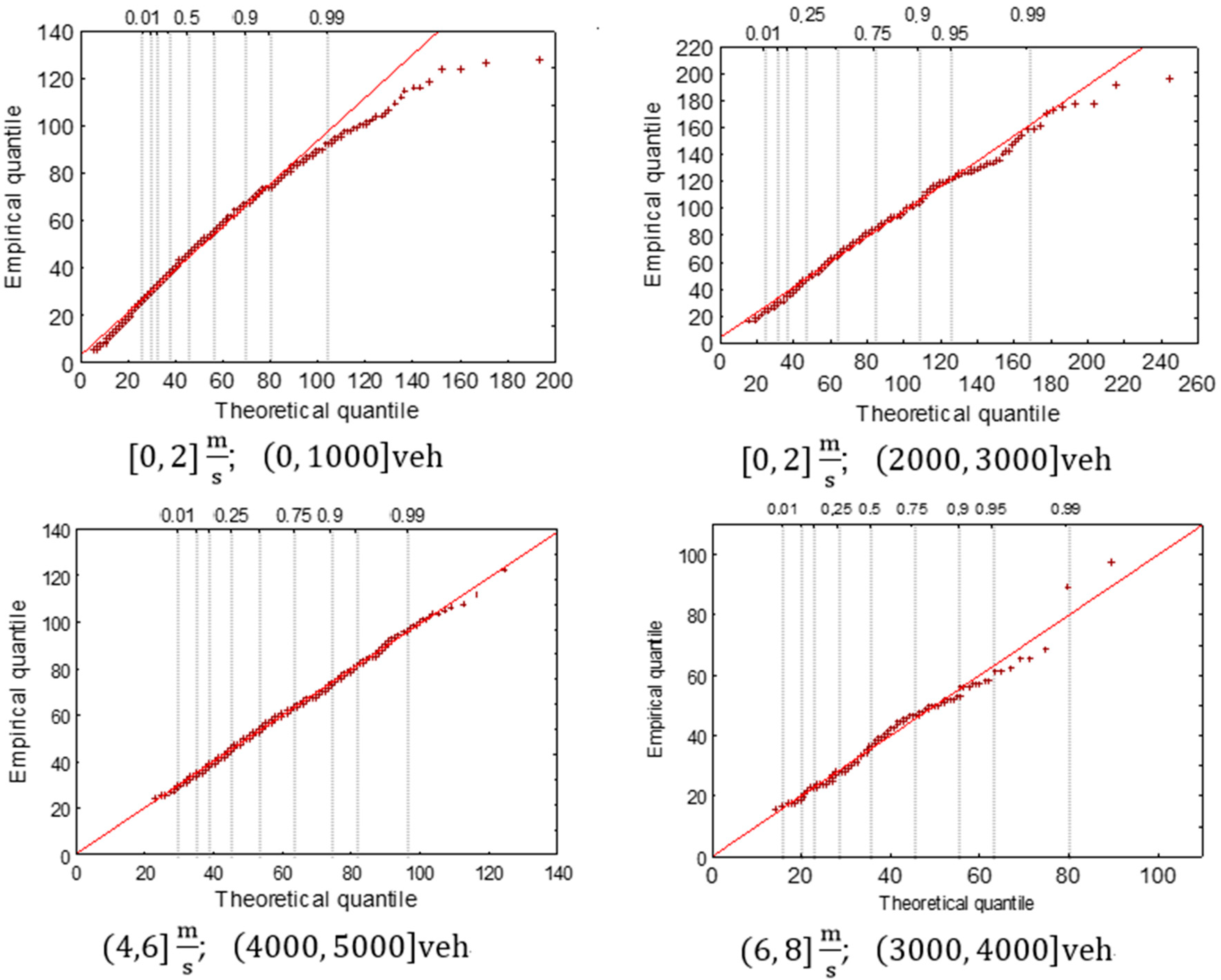
Both statistical tests indicated a lack of conformity to the log-normal distribution in one case only: For the lightest wind conditions—[0, 2] m/s—and the lowest traffic levels—(0, 1000] vehicles. This is the largest of the clusters. If the clusters are labelled according to their position in the matrix, this is cluster (1, 1). In three cases the ${\chi }^2$ test indicated a lack of conformity to the theoretical distribution (rejection of the null hypothesis H₀) while the Kolmogorov–Smirnov test indicated of the lack of grounds to reject H₀. To make a final determination of the possibility of identifying the empirical distribution with the appropriate theoretical distribution, Q-Q (quantile-quantile) plots were produced and used to assess the deviation between the distributions. The Q-Q plots for the clusters for which the applied test statistics indicated a rejection of the hypothesis H₀ (green fields in Table 4) are shown in Figure 5. The largest deviations from the theoretical distribution are found for high concentration values; clearly the greatest differences occurred for cluster (1, 1) ($\left[0, 2\right]\frac{\mathrm{m}}{\mathrm{s}}$; $\left(0, 1000\right]$ veh). Caution must therefore be applied when interpreting the subsequent results with respect to the lowest values of wind speed and traffic flow. Nonetheless, these are conditions that occur mainly at night, when NO₂ concentrations are relatively low. In the remaining 23 cases, both tests confirmed the conformity of the empirical distribution of NO₂ concentrations to the log-normal distribution.

Empirical histograms, along with a graph of the density function of the fitted theoretical distribution, are shown in Figure 6. The arrangement of the histograms is in accordance with the matrix arrangement of Table 3. All of them are characterized by right-handed asymmetry. The kurtosis of the distribution increases as the wind speed increases, and falls as the traffic flow increases.

3.2. Forecasting the Probability

Using knowledge of the theoretical distributions of NO₂ concentrations given the tabulated ambient conditions, probabilities were computed for the exceeding of defined concentration values in each of the clusters representing defined conditions (

Table 5. Probabilities of the exceeding of given NO₂ concentrations, times for which those values are exceeded in days of the year (in round brackets) and period of repeatability of the event in years [in square brackets].

$\mathit{P}(\mathit{Y}>40\frac{\mathsf{\mu }\mathbf{g}}{{\mathbf{m}}^3})$	$\left[0,2\right]$	$\left(2,4\right]$	$\left(4,6\right]$	$\left(6,8\right]$	$\left(8,+\mathit{\infty }\right)$
(0, 1000]	39.1% (143)	23.7% (86)	14.2% (52)	7.4% (27)	3.2% (12)
(1000, 2000]	64.5% (235)	48.9% (178)	34.0% (124)	22.3% (81)
(2000, 3000]	74.6% (272)	59.0% (215)	46.7% (170)	36.2% (132)	17.9% (65)
(3000, 4000]	79.4% (290)	64.2% (234)	54.7% (200)	41.9% (153)	27.8% (101)
(4000, 5000]	82.5% (301)	77.1% (281)	71.4% (261)	63.8% (233)	52.8% (193)
(5000, $+\infty$)	85.7% (313)	81.0% (295)	74.4% (272)	66.5% (243)
$\mathit{P}(\mathit{Y}\mathbf{>}\mathbf{100}\frac{\mathsf{\mu }\mathbf{g}}{{\mathbf{m}}^{\mathbf{3}}})$	$\mathbf{\left[}\mathbf{0}\mathbf{,}\mathbf{2}\mathbf{\right]}$	$\mathbf{\left(}\mathbf{2}\mathbf{,}\mathbf{4}\mathbf{\right]}$	$\mathbf{\left(}\mathbf{4}\mathbf{,}\mathbf{6}\mathbf{\right]}$	$\mathbf{\left(}\mathbf{6}\mathbf{,}\mathbf{8}\mathbf{\right]}$	$\mathbf{\left(}\mathbf{8}\mathbf{,}\mathbf{+}\mathbf{\infty }\mathbf{\right)}$
(0, 1000]	5.5% (20)	2.1% (8)	1.0% (4)	0.4% (1)	0.1% (<1)
(1000, 2000]	14.7% (54)	7.7% (28)	4.0% (15)	2.0% (7)
(2000, 3000]	22.6% (82)	12.0% (44)	6.2% (23)	4.4% (16)	1.1% (4)
(3000, 4000]	15.8% (58)	12.0% (44)	8.0% (29)	3.9% (14)	2.2% (8)
(4000, 5000]	19.2% (70)	14.1% (51)	10.6% (39)	7.3% (27)	6.2% (23)
(5000, $+\infty$)	19.4% (71)	15.0% (55)	11.7% (43)	7.8% (28)
$\mathit{P}(\mathit{Y}\mathbf{>}\mathbf{200}\frac{\mathsf{\mu }\mathbf{g}}{{\mathbf{m}}^{\mathbf{3}}})$	$\mathbf{\left[}\mathbf{0}\mathbf{,}\mathbf{2}\mathbf{\right]}$	$\mathbf{\left(}\mathbf{2}\mathbf{,}\mathbf{4}\mathbf{\right]}$	$\mathbf{\left(}\mathbf{4}\mathbf{,}\mathbf{6}\mathbf{\right]}$	$\mathbf{\left(}\mathbf{6}\mathbf{,}\mathbf{8}\mathbf{\right]}$	$\mathbf{\left(}\mathbf{8}\mathbf{,}\mathbf{+}\mathbf{\infty }\mathbf{\right)}$
(0, 1000]	0.5% (2)	0.1% (<1) [2]	0.1% (<1) [5]	0.0% (<1) [17]	0.0% (<1) [82]
(1000, 2000]	1.7% (6)	0.7% (2)	0.3% (1)	0.1% (<1) [2]
(2000, 3000]	3.4% (12)	1.3% (5)	0.4% (2)	0.3% (1)	0.0% (<1) [7]
(3000, 4000]	0.9% (3)	1.0% (4)	0.5% (2)	0.2% (1)	0.1% (<1)
(4000, 5000]	1.3% (5)	0.7% (3)	0.4% (2)	0.2% (1)	0.3% (1)
(5000, $+\infty$)	1.0% (4)	0.7% (3)	0.5% (2)	0.2% (1)
$\mathit{P}(\mathit{Y}\mathbf{>}\mathbf{400}\frac{\mathsf{\mu }\mathbf{g}}{{\mathbf{m}}^{\mathbf{3}}})$	$\mathbf{\left[}\mathbf{0}\mathbf{,}\mathbf{2}\mathbf{\right]}$	$\mathbf{\left(}\mathbf{2}\mathbf{,}\mathbf{4}\mathbf{\right]}$	$\mathbf{\left(}\mathbf{4}\mathbf{,}\mathbf{6}\mathbf{\right]}$	$\mathbf{\left(}\mathbf{6}\mathbf{,}\mathbf{8}\mathbf{\right]}$	$\mathbf{\left(}\mathbf{8}\mathbf{,}\mathbf{+}\mathbf{\infty }\mathbf{\right)}$
(0, 1000]	0.02% [16]	0.00% [88]	0.00% [206]	0.00% [880]	0.00% [>1000]
(1000, 2000]	0.07% [4]	0.02% [13]	0.01% [33]	0.00% [87]
(2000, 3000]	0.19% (1) [1]	0.05% [6]	0.01% [30]	0.01% [33]	0.00% [462]
(3000,4000]	0.01% [32]	0.02% [12]	0.01% [26]	0.00% [141]	0.00% [164]
(4000, 5000]	0.02% [17]	0.01% [42]	0.00% [81]	0.00% [190]	0.00% [79]
(5000, $+\infty$)	0.01% [36]	0.00% [63]	0.00% [81]	0.00% [215]

). The values in the table should be interpreted in the following manner: Given a traffic flow not exceeding 1000 vehicles and a wind speed not greater than 2 m/s, the probability that the atmospheric concentration of NO₂ will exceed 40 μg/m³ is 39.1%. The probability of the occurrence of a given concentration of NO₂ decreases as its value increases. The probabilities are highest for the exceeding of the smallest values. The probability of exceeding a concentration of 40 μg/m³ given the least favorable conditions (cluster (6, 5): Traffic flow > 5000 vehicles, wind speed $\le$ 2 m/s) is above 85%, which means that statistically, this concentration is exceeded for 7507 out of the 8760 h in a year. Because the atmospheric NO₂ concentration is subject to significant variation in the course of a day, the accepted safe value is exceeded every day. With a fall in traffic flow and an increase in wind speed, the probability of exceeding the mean annual permissible value falls to 3.2% for cluster (1, 5), equivalent to 282 h in a year. The probabilities of concentrations in excess of 100 μg/m³ are several times smaller: They range from 0.1% (value exceeded for 10 h in a year) for conditions with strong wind and low traffic flow, i.e., cluster (1, 5), to 22.6% (value exceeded for 1997 h in a year) for cluster (3, 1), with traffic flow in the interval (2000, 3000] and wind speed not exceeding 2 m/s.

The determined probability distributions indicate that for 7 of the 28 described sets of ambient conditions, the permissible value of the NO₂ concentration (200 μg/m³) is reached less frequently than once per year. In unfavorable ambient conditions—cluster (3, 1)—the permissible level may be exceeded with a probability of 3.4% (300 h in a year). The probability of exceeding the alarm level of 400 μg/m³ is always lower than 0.2%. The largest probabilities of NO₂ concentrations exceeding 100, 200 and 400 μg/m³ were identified in the case of cluster (3, 1), with low wind speeds ($\le$2 m/s) and traffic flows in the interval (2000, 3000] vehicles. This cluster contains a total of 985 cases, mainly from the evening hours (70% of cases occur from 20:01 to 22:00) when the pollutants emitted by traffic throughout the day remain accumulated, although the traffic flow at that time is not especially high. A low wind speed increases the accumulation of pollutants and favors the occurrence of chemical reactions. During volatile organic compounds degradation processes, apart from ozone formation, the transformation of NO to NO₂ also occurs. This process is more intense when more substrates are present in the air and when the atmospheric conditions are more favorable, particularly when there is low wind.

Probabilities of exceeding given values were found to decrease more rapidly with an increase in wind speed than with a fall in traffic volume. The very strong influence of wind speed on atmospheric NO₂ concentration is largely a result of the geographic location of the intersection. Given Wrocław’s prevailing WNW winds, the alignment of the intersection with the wind direction favors the evacuation of pollutants. The surrounding buildings modify the wind speed and direction only to a small degree.

3.3. Verification

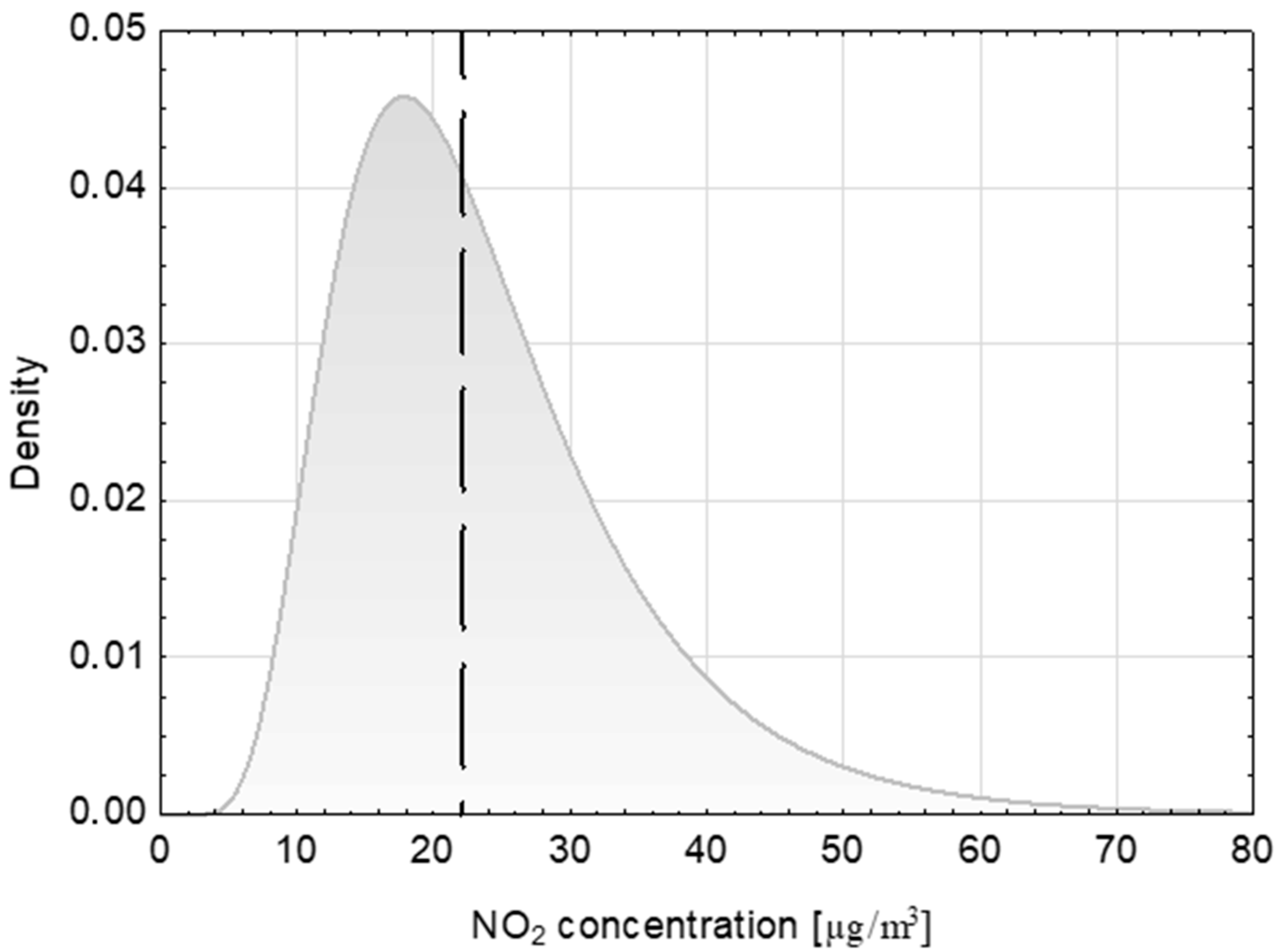
The above method of probabilistic forecasting of atmospheric NO₂ conditions was subjected to verification using independent data from the first six months of 2018. The values of NO₂ concentrations from the verification period were partitioned into clusters according to the key described in Section 3.1. There were 2586 h in which the concentration exceeded 40 μg/m³. The value was above 100 μg/m³ only for 41 h, which made verification impossible due to the low frequencies of occurrence within clusters. No cases of concentrations in excess of 200 μg/m³ were recorded. The statistical significance of the differences between the obtained frequencies of NO₂ concentrations in excess of 40 μg/m³ for the whole matrix compared with the frequency matrix for 2015–2017 was investigated using the t-test. On this basis, for a significance level of 0.05, the hypothesis of equality of means for the frequencies can be accepted (p-value = 0.86), which means that the determined frequencies of occurrence also give a good description of the independent data from 2018. An example forecast, in the form of a density function graph for a computed log-normal distribution and the actual value for the time 13:00 on 18 March 2018, is shown in Figure 7. At that time the recorded wind speed was 10 m/s, and the traffic flow was 2891 vehicles. These values correspond to cluster (3, 5) in the matrix of Table 3. The actual recorded NO₂ concentration was 22 μg/m³.

For the quantitative evaluation of forecast resolution and uncertainty, the continuous rank probability score (CRPS) was used. This is designed to evaluate the reliability, resolution and uncertainty of probabilistic forecasts [42,43]. The CRPS value for a single forecast (hour) ranged from 1.38 to 53.2 μg/m³, with a mean of 9.15 μg/m³. Considering the simplicity of the applied forecasting method and its precision (hourly), this result may be considered satisfactory. Balashov et al. [22], analysing their complex REGiS model for forecasting daily ozone concentrations, obtained mean CRPS values ranging from 3.6 to 6.3 ppbv.

Mean CRPS values were also obtained for the clusters. The largest errors occurred in the forecasting of concentrations for the lightest winds (

Table 6. Continuous rank probability score (CRPS) for clusters.

$\mathit{C}\mathit{R}\mathit{P}\mathit{S}[\mathsf{\mu }\mathbf{g}/{\mathbf{m}}^3]$	$\left[0,2\right]$	$\left(2,4\right]$	$\left(4,6\right]$	$\left(6,8\right]$	$\left(8,+\mathit{\infty }\right)$
(0, 1000]	9.1	7.6	5.8	4.1	2.1
(1000, 2000]	10.2	10.2	7.7	7.0	4.0
(2000, 3000]	12.5	11.4	6.7	7.3	4.2
(3000, 4000]	12.2	9.9	9.1	7.2	6.4
(4000, 5000]	10.1	9.6	7.4	6.0	5.7
(5000, $+\infty$)	9.5	7.3	8.3	6.8	3.8

). The phenomenon of accumulation of pollutants, which occurs at the lowest wind speeds, and is significantly influenced by values from past time points, is not taken into account in the model (by design). For wind speeds above 4 m/s, the CRPS takes single-figure values. Verification of the model using independent data confirmed the effectiveness of the cluster-based model for probabilistic forecasting of pollutant concentrations on a major transport route.

4. Conclusions

This article has presented a cluster-based approach to the problem of probabilistic forecasting of concentrations of nitrogen dioxide on a major transport route. It was shown to be most effective to consider the impact of traffic flow and wind speed on NO₂ concentrations using a matrix-based partitioning of ambient conditions. For each cluster, corresponding to an interval of wind speeds and an interval of traffic flow values, parameters were calculated for log-normal distributions of NO₂ concentrations. Based on the obtained probability density functions of the theoretical distributions, probabilities were computed for the occurrence of NO₂ concentrations in excess of 40 μg/m³, 100 μg/m³, 200 μg/m³ and 400 μg/m³. The probability that the mean annual permissible atmospheric NO₂ concentration will be exceeded is as high as 85.7% assuming the highest traffic volume (in excess of 5000 vehicles) and very low wind speed (not greater than 2 m/s). For higher boundary values, the phenomenon of accumulation of pollutants was observed to become more significant. The fact that the cluster containing moderate traffic flows of (2000, 3000] vehicles gives the highest probabilities of exceeding the concentrations 100 μg/m³, 200 μg/m³ and 400 μg/m³ is a consequence of the time of day to which these cases correspond: Most of them are from the hours 20:01–22:00. Verification of the model using independent data from the first six months of 2018 demonstrated statistically significant conformity of the frequencies of occurrence of NO₂ concentrations for the tabulated conditions. The mean prediction error measured by the CRPS was 9.15 μg/m³. Analysis of the probabilities of exceeding the permissible and alarm levels of NO₂ concentration showed that a reduction in the number of vehicles must be significant to achieve a noticeable reduction in NO₂ levels along the transport route. With an increase in wind speed, the probability that a given nitrogen oxide concentration threshold will be exceeded is reduced approximately by half for every 2 m/s. Thus, a significant contribution to the removal of pollutants comes from the movement of air through the city, and consequently from the sustainable nature of its building development.

The main limitation on the applicability of the presented methodology is that it is point-based. When a forecast is generated in this form, it is not possible to extend it to a wider area. Further work will investigate the possibility of extending probabilistic forecasting by the cluster method to several points located along the route, and then extending the forecast to the entire length of the road. A further goal of future work will be the identification of partition points for the explanatory variables in an optimization process: For example, minimization of the variance within a cluster.

References

- Olvera Alvarez, H.A.; Myers, O.B.; Weigel, M.; Armijos, R.X. The value of using seasonality and meteorological variables to model intraurban PM2.5 variation. Atmos. Environ. 2018, 182, 1–8. [Google Scholar] [CrossRef] [PubMed]
- Catalano, M.; Galatioto, F.; Bell, M.; Namdeo, A.; Bergantino, A.S. Improving the prediction of air pollution peak episodes generated by urban transport networks. Environ. Sci. Policy 2016, 60, 69–83. [Google Scholar] [CrossRef]
- Donnelly, A.; Misstear, B.; Broderick, B. Real time air quality forecasting using integrated parametric and non-parametric regression techniques. Atmos. Environ. 2015, 103, 53–65. [Google Scholar] [CrossRef] [Green Version]
- Bertaccini, P.; Dukic, V.; Ignaccolo, R. Modeling the Short-Term Effect of Traffic and Meteorology on Air Pollution in Turin with Generalized Additive Models. Adv. Meteorol. 2012, 2012, 609328. [Google Scholar] [CrossRef]
- Shi, J.P.; Harrison, R.M. Regression modelling of hourly NOx and NO2 concentration in urban air in London. Atmos. Environ. 1997, 31, 4081–4094. [Google Scholar] [CrossRef]
- Aldrin, M.; Haff, I.H. Generalized additive modelling of air pollution, traffic volume and meteorology. Atmos. Environ. 2005, 39, 2145–2155. [Google Scholar] [CrossRef]
- Zhang, Z.; Zhang, X.; Gong, D.; Quan, W.; Zhao, X.; Ma, Z.; Kim, S.-J. Evolution of Surface O3 and PM2.5 concentrations and their relationships with meteorological conditions over the last decade in Beijing. Atmos. Environ. 2015, 108, 67–75. [Google Scholar] [CrossRef]
- Battista, G.; de Lieto Vollaro, R. Correlation between air pollution and weather data in urban areas: Assessment of the city of Rome (Italy) as spatially and temporally independent regarding pollutants. Atmos. Environ. 2017, 165, 240–247. [Google Scholar] [CrossRef]
- Elangasinghe, M.A.; Singhal, N.; Dirks, K.N.; Salmond, J.A. Development of an ANN–based air pollution forecasting system with explicit knowledge through sensitivity analysis. Atmos. Pollut. Res. 2014, 5, 696–708. [Google Scholar] [CrossRef]
- Nejadkoorki, F.; Baroutian, S. Forecasting extreme PM10 concentrations using artificial neural networks. Int. J. Environ. Res. 2012, 6, 277–284. [Google Scholar] [CrossRef]
- Papanastasiou, D.K.; Melas, D.; Kioutsioukis, I. Development and assessment of neural network and multiple regression models in order to predict PM10 levels in a medium–sized Mediterranean city. Water Air Soil Pollut. 2007, 182, 325–334. [Google Scholar] [CrossRef]
- Singh, K.P.; Gupta, S.; Rai, P. Identifying pollution sources and predicting urban air quality using ensemble learning methods. Atmos. Environ. 2013, 80, 426–437. [Google Scholar] [CrossRef]
- Kamińska, J.A. The use of random forests in modelling short-term air pollution effects based on traffic and meteorological conditions: A case study in Wrocław. J. Environ. Manag. 2018, 217C, 164–174. [Google Scholar] [CrossRef] [PubMed]
- Laña, I.; Del Ser, J.; Pedró, A.; Vélez, M.; Casanova-Mateo, C. The role of local urban traffic and meteorological conditions in air pollution: A data-based study in Madrid, Spain. Atmos. Environ. 2016, 145, 424–438. [Google Scholar] [CrossRef]
- Sayegh, A.; Tate, J.A.; Ropkins, K. Understanding how roadside concentrations of NOx are influenced by the background levels, traffic density, and meteorological conditions using Boosted Regression Trees. Atmos. Environ. 2016, 127, 163–175. [Google Scholar] [CrossRef]
- Kamińska, J.A. Residuals in the modelling of pollution concentration depending on meteorological conditions and traffic flow, employing decision trees. ITM Web Conf. 2018, 23, 00016. [Google Scholar] [CrossRef]
- Larkin, A.; Geddes, J.A.; Martin, R.V.; Xiao, Q.; Liu, Y.; Marshall, J.D.; Brauer, M.; Hystad, P. Global Land Use Regression Model for Nitrogen Dioxide Air Pollution. Environ. Sci. Technol. 2017, 51, 6957–6964. [Google Scholar] [CrossRef] [PubMed]
- Kamińska, J.A. A random forest partition model for predicting NO2 concentrations from traffic flow and meteorological conditions. Sci. Total Environ. 2019, 651, 475–483. [Google Scholar] [CrossRef] [PubMed]
- Aznarte, J.L. Probabilistic Forecasting for extreme NO2 pollution episodes. Environ. Pollut. 2017, 229, 321–328. [Google Scholar] [CrossRef] [PubMed]
- Koenker, R. Quantile Regression, No. 38 in Econometric Society Monographs; Cambridge University Press: Cambridge, UK, 2005. [Google Scholar]
- Air Pollution and Biometeorological Forecast and Information System (LIFE-APIS/PL). Available online: http://life-apis.meteo.uni.wroc.pl/en/ (accessed on 14 November 2018).
- Balashov, N.V.; Thompson, A.M.; Young, G.S. Probabilistic forecasting of surface ozone with a novel statistical approach. J. Appl. Meteorol. Climatol. 2017, 56, 297–316. [Google Scholar] [CrossRef]
- Garner, G.G.; Thompson, A.M. Ensemble statistical post-processing of the National Air Quality Forecast Capability: Enhancing ozone forecast in Boltimore, Maryland. Atmos. Environ. 2013, 81, 517–522. [Google Scholar] [CrossRef]
- Padró-Martínez, L.T.; Patton, A.P.; Trull, J.B.; Zamore, W.; Brugge, D.; Durant, J.L. Mobile monitoring of particle number concentration and other traffic-related air pollutants in a near-highway neighborhood over the course of a year. Atmos. Environ. 2012, 61, 253–264. [Google Scholar] [CrossRef] [PubMed] [Green Version]
- Beckerman, B.; Jerrett, M.; Brook, J.R.; Verma, D.J.; Arain, M.A.; Finkelstein, M.M. Correlation of Nitrogen Dioxide with Other Traffic Pollutants near a Major Expressway. Atmos. Environ. 2008, 42, 275–290. [Google Scholar] [CrossRef]
- González-Aparicio, I.; Hidalgo, J.; Baklanov, A.; Padró, A.; Santa-Coloma, O. An hourly PM10 diagnosis model for the Bilbao metropolitan area using a linear regression methodology. Environ. Sci. Pollut. Res. 2013, 20, 4469–4483. [Google Scholar] [CrossRef] [PubMed]
- Zhang, K.; Batterman, S. Air pollution and health risks due to vehicle traffic. Sci. Total Environ. 2013, 450, 307–316. [Google Scholar] [CrossRef] [PubMed] [Green Version]
- Mlakar, P.; Boinar, M. Perception neutral network-based model predicts air pollution. In Proceedings of the Intelligent Information Systems 1997, Grand Bahama Island, Bahamas, 8–10 December 1997; pp. 345–349. [Google Scholar]
- Keeler, R.H. A Machine Learning Model of Manhattan Air Pollution at High Spatial Resolution. Ph.D. Thesis, Massachusetts Institute of Technology, Cambridge, MA, USA, 2014. [Google Scholar]
- Breiman, L. Random Forests. Mach. Learn. 2001, 45, 5–32. [Google Scholar] [CrossRef] [Green Version]
- Breiman, L. Statistical modelling: The two cultures (with comments and a rejoinder by the author). Statist. Sci. 2001, 16, 199–231. [Google Scholar] [CrossRef]
- Dunea, D.; Iordache, S.; Alexandrescu, D.-C.; Dincă, N. Screening the weekdays/weekend patterns of air pollutant concentrations recorded in southeastern Romania. Environ. Eng. Manag. J. 2014, 13, 3105–3114. [Google Scholar] [CrossRef]
- Barratt, B.; Atkinson, R.; Ross Anderson, H.; Beevers, S.; Kelly, F.; Mudway, L.; Wilkinson, P. Investigation into the use of the CUSUM technique in odentyfying changes in mean air pollution levels following introduction for a traffic management scheme. Atmos. Environ. 2007, 41, 1784–1791. [Google Scholar] [CrossRef]
- Kazak, J.; Chalfen, M.; Kamińska, J.; Szewrański, S.; Świąder, M. Geo-Dynamic Decision Support System for Urban Traffic Management. In Lecture Notes in Geoinformation and Cartpgraphy; Ivan, I., Horak, J., Inspektor, T., Eds.; Dynamics in GIScience. GIS Ostrava 2017; Springer: Cham, Switzerland, 2018; pp. 195–207. [Google Scholar]
- Chalfen, M.; Kamińska, J.A. Identification of parameters and verification of an urban traffic flow model. A case study in Wrocław. ITM Web Conf. 2018, 23, 00005. [Google Scholar] [CrossRef]
- Szewrański, S.; Kazak, J.; Żmuda, R.; Wawer, R. Indicator-based assessment for soil resource management in the Wrocław larger urban zone of Poland. Pol. J. Environ. Stud. 2017, 26. [Google Scholar] [CrossRef]
- Tokarczyk-Dorociak, K.; Kazak, J.; Szewrański, S. The impact of a large city on land use in suburban area—The case of Wrocław (Poland). J. Ecol. Eng. 2018, 19. [Google Scholar] [CrossRef]
- Kiełkowska, J.; Tokarczyk-Dorociak, K.; Kazak, J.; Szewrański, S.; van Hoof, J. Urban Adaptation to Climate Change Plans and Policies—The Conceptual Framework of a Methodological Approach. J. Ecol. Eng. 2018, 19, 50–62. [Google Scholar] [CrossRef]
- Kazak, J.; van Hoof, J.; Szewranski, S. Challenges in the wind turbines location process in Central Europe—The use of spatial decision support systems. Renew. Sustain. Energy Rev. 2017, 76. [Google Scholar] [CrossRef]
- Aczel, A.D. Complete Business Statistics, 2nd ed.; Richard D. Irvin, Inc.: Homewood, IL, USA, 1993. [Google Scholar]
- Rozporządzenie Ministra Środowiska z Dnia 24 Sierpnia 2012 r. w Sprawie Poziomów Niektórych Substancji w Powietrzu. (Regulation of the Minister of Environment of 14 August 2012 on Levels of Certain Substances in the Air). (Dz.U.2012.1031); 2012. Available online: http://prawo.sejm.gov.pl/isap.nsf/download.xsp/WDU20120001031/O/D20121031.pdf (accessed on 14 November 2018).
- Hersbach, H. Decomposition of the Continuous Ranked Probability Score for Ensemble Prediction. Syst. Weather Forecast. 2000, 15, 559–570. [Google Scholar] [CrossRef]
- Baran, S.; Lerch, S. Log-normal distribution based Ensemble Model Output Statistics model for probabilistic wind-speed forecasting. Q. J. R. Meteorol. Soc. 2015, 141, 2289–2299. [Google Scholar] [CrossRef]
Figure 1.
Traffic, air and meteorological monitoring sites in Wrocław: The Hallera traffic counter (blue), pollution stations (red) and meteorological station (yellow).
Figure 2.
Frequency histogram of atmospheric NO2 concentrations at the Hallera–Powstańców Śląskich intersection in 2015–2017.
Figure 3.
Box plots of traffic at the Hallera–Powstańców Śląskich intersection for different time scales.
Figure 4.
Histogram and Wind Rose for Wrocław Strachowice meteorological station in 2015–2017.
Figure 5.
Q-Q plots for NO2 concentration in selected clusters.
Figure 6.
Empirical histograms and fitted density functions of log-normal distributions for each cluster.
Figure 7.
An example of the forecast for 18 March 2018 (14:00).