Multi-Criteria Analysis of Pollution Caused by Auto Traffic in a Geographical Area Limited to Applicability for an Eco-Economy Environment

Abstract

The pollution caused by road traffic is a significant problem for society in the 21st century. Climate change and mortality among the population, are increasingly influenced by increasing traffic in urban agglomerations. The present study aims at the multi-criteria analysis of the pollution caused by traffic at several busy intersections in the city of Sibiu, Romania. Classification of intersections was done using the Synchro Studio with Warrants software. Air pollutants, noise, and the number of vehicles in the traffic were taken into account. To analyze these criteria as a whole, the analytical hierarchy process (AHP) and technique for order preference by similarity to ideal solution (TOPSIS) methods were used. A comparative study has been undertaken on the results obtained by applying the two multicriteria methods. The paper aims to provide solutions for the eco-economy of the future.

1. Introduction

The pursuit of continuous economic growth simultaneously with the existence of a living planet is not possible. Endemic economic growth will inevitably lead to an ecological recession that becomes unfortunate for the inhabitants of the planet when limits are exceeded.

Consumption-based economic growth appears to jeopardize the current estimated population of 7.6 billion, but more than that, it will not be able to ensure a fair life and sustainable development for the 9 billion expected to be registered by the year 2040. The current market economy shows many errors, and proves to be performing poorly for most of the planet’s inhabitants in terms of exhausting the environment.

The origin of the term “eco-economy” belongs to the American scientist Lester R. Brown. He named one of his fundamental works “Eco-Economy: Building an Economy for the Earth,” a work that was first printed in the United States in 2001. The etymology of the word “eco” from “economy” is rooted in the Greek oikos, which designates a house, a household, a habitat, a fortress, and nomos, which means law, that is, the laws governing a fortress or a household. In fact, the eco-economy that resembles the ecological economy is the expression of the recognition of the existence not only of economic realities but, of interdependence with multiple objective interactions between the economic system and the ecological system.

“We know the kind of restructuring that is needed. In simplest terms, our fossil-fuel-based, automobile-centered, throwaway economy is not a viable model for the world. The alternative is a solar/hydrogen energy economy, an urban transport system that is centered on advanced-design public rail systems and that relies more on the bicycle and less on the automobile, and a comprehensive reuse/recycle economy.”

[1]

Fierce international competition causes this most of the time. The environment is exhausted and the resources exploited abusively as if there were no tomorrow or a growing population on the planet. It is natural that under these circumstances, more people than ever are worried about the future. If any natural system works cyclically, it means that what rises from earth, should be returned properly forming the basis of a new cycle. The same cannot be said about the current economy which produces more and more, disregarding the natural life cycle and polluting our planet with un-recycled waste. So, if this is increasingly alarming, we should not ask for more from the system, but need to find solutions for sustainable change and refinement.

Today, economic growth remains the desideratum of nations, and world supremacy is measured mainly by gross domestic product (GDP). Under these circumstances, the cycle we talked about in the previous passage is increasingly far from being metabolized and sustaining life at acceptable standards on the planet. A popular system generates economic growth at all costs, and will turn against humanity and turn rich into poor people, or can even accelerate the pace of growth of mortalities caused by premature deaths due to poor air quality.

Among the main causes leading to deaths caused by pollution, it must be noted that the most toxic substances are fine particles (PM2.5—particulate diameter less than 2.5 microns) which kill 428,000 people in Europe, including 399,000 in the European Union (EU). Long-range nitrogen dioxide (78,000 victims) and ozone (14,000 casualties).

To estimate the number of people who have died from air pollution or any other pollution is not an easy task.

Breathing ultra-fine particles and toxic gases can increase the chances of dying prematurely, as it causes respiratory and cardiovascular problems. Fortunately, scientists worldwide have worked to estimate this, and a study by the Max Planck Institute for Chemistry and the London School of Hygiene and Tropical Medicine provides figures on people who died due to pollution.

According to the research, 4.5 million people died prematurely due to air pollution-related diseases (including 237,000 children under five years of age due to respiratory diseases) in 2015 alone. The study is published in the journal The Lancet: Planetary Health.

This means that on average 12,329 people died daily. If you report the total number of people killed annually in road accidents (1.3 million), the figure is 3.5 times less than the number of people dying from polluted air [2].

So, if a few decades ago the world was worried about the large number of deaths due to traffic accidents resulting in the introduction of increased safety measures, these statistics show that the alarm signal should sound stronger for pollution.

Even though pollution has been reported for a very long time and the world has been warned of its dangers, it seems to be inadequate and studies must continue to be documented and vehement in the hope that companies, and especially governments, will be aware of the danger and take necessary action on the case.

Another important annual report on global air conditions has recently been published by the Institute for Health Effects (HEI), and found that more than 95% of the world’s population breathes unhealthy air. Long-term exposure to air pollution has contributed to the deaths of more than 6 million people in 2016 caused by strokes, heart attacks, lung diseases, and pulmonary cancer.

Air pollution is now the fourth most significant cause of death worldwide with most of the deaths in poorer countries. The underlying study can be extended to any area or road junction, and can be an essential step in bringing institutions and populations the awareness of the dangers that may result from an unsustainable economy.

If progress depends on materialistic values, such as popularity, image, and financial success, all this may no longer hold its value when life is threatened. So, while progress is being pursued, it is increasingly clear that it cannot be recorded at any cost, but only with a sustainable economy: an eco-bio-economy. The more communities respect these principles, the more they can have a longer and happier life.

There are several ways to perform procedures assessing the environmental impact of pollutants. Verification lists, matrix or network techniques, geographic information system (GIS) methods and quantitative methods can be used to assess the environmental impact and reach a final conclusion [3]. It should be emphasized that there is no single or distinct method. The user has to decide which methods are to be used in the project.

The environmental impact assessment (EIA) is a procedure for assessing the environmental implications of a decision to enact legislation, to implement policies and plans, or to initiate development projects. It has become a widely accepted tool for environmental management. EIA is an intrinsically complex multi-dimensional process. In fact, the process of EIA has been evolving ever since it was adopted for analyzing the environmental impacts of developmental projects [4]. EIA is the assessment of the possible impact that a proposed plan or project may have on the environment, together consisting of the natural, social and economic aspects [5].

Ten criteria in environment, economy, society-politic, and technology dimensions were employed to achieve sustainability measurement (SM) of WT processes. The multi-criteria sustainability assessment method allow different experts to attend the SM, and enable the participants to employ the natural language/words to depict their intuitionistic opinions [6].

Since there is increasing pressure to quantify the impact on the environment, quantitative methods have been considered as beneficial methods because they are able to compare different alternatives to a project. The analytical hierarchy process (AHP) and technique for order preference by similarity to ideal solution (TOPSIS) multi-criteria methods can be used successfully to evaluate different factors involved in environmental processes.

A new multi-criteria method is proposed in 2018: “The intuitionistic fuzzy AHP (IFAHP)” method. For the Fuzzy delphi method, the judgments of experts and representatives on criterion weights are made by linguistic variables and quantified by intuitionistic fuzzy theory, which is also used to weigh the importance of experts and representatives. This process generates the entropy weights of criteria, which are combined with indices values and weights to rank the alternatives by the fuzzy AHP method [7].

Among quantitative methods for assessing the environmental impact of pollutants, the Battelle–Columbus method can be mentioned. This method should be mentioned if an environmental impact unit is defined based on the environmental quality index and the importance of the unit of environmental parameters. Quantitative methods define a numerical value that quantifies the state of the environment. Quantitative methods are diverse. These quantitative methods can be used to assess the quality of the environment in a complex way and are able to assess the impact of human activities on the environment and to develop mitigation plans for the rehabilitation of the polluted environment. The method will be applied for the first time on the measurements made on the physicochemical factors in the city of Sibiu and its geographical region.

The link between parameters defining air quality can be analyzed at this time using the Pearson method that performs a correlated analysis between these parameters.

One of the objectives of our project is to focus on just one element of the air, namely breathable air, and to produce concrete results using a quantitative method for assessing it in accordance with the EU guidelines and the Framework Directive concerning air [8].

The following parameters will be measured in accordance with the Romanian Standards:

• CO carbon monoxide;
• Nitrogen oxides NOx;
• Fine dust PM 10
• Ozone concentration;
• Hydrocarbon emissions;
• Noise;
• Number of vehicles.

The main objective of this paper is to determine the most polluted and least polluted intersections, depending on the multiple factors taken into account and analyzed using the AHP and TOPSIS multichannel methods.

The methods will be applied for the first time on the measurements made on the physicochemical factors at the intersections considered from the city of Sibiu. The link between parameters defining air quality can be analyzed at this time using the Pearson method that performs a correlated analysis between these parameters.

One of the objectives of our project is to focus only on one element of the air i.e., the air at the intersections analyzed, and to obtain concrete results using two quantitative methods of its evaluation in accordance with the EU guidelines and the Air Framework Directive [8].

The algorithm presented in this paper will contain the following steps:

• Intersection classification using Synchro software;
• Determining the parameters to be considered for each intersection;
• Calculation of the weight of each pollutant parameter using the AHP method;
• Classification of intersections using the TOPSIS multicriteria method, taking into account the weights of the pollutants obtained in the AHP method.

2. Materials and Methods

The multi-criteria analysis method (MCDM) emerged in the 1960s as a decision-making tool. Recently, it has become increasingly popular in project management, both in ex-ante and ex-post evaluation of projects, as shown by [9]. Multi-criteria analysis applies in particular to cases where the one-criterion approach is not sufficient (as is the case with cost-benefit analysis), especially when significant monetary and social impacts cannot be converted into monetary values. The purpose of this tool is to structure and combine the various assessments that need to be taken into account in the decision-making process where more choice is made in the decision-making process and the treatment applied to each of them greatly determines the final decision.

Importantly, multi-criteria analysis is used to highlight the rationale and subjective views of stakeholders in relation to each problem. It is usually used to synthesize opinions expressed, prioritize structures, analyze conflict situations, make recommendations, and/or provide operational advice.

Generally, the MCDM method is composed of five components: the objective, the preferences of the decision maker, the alternatives, the criteria, and the results.

Multi-criteria methods can be classified as in Figure 1.

Multi-criteria models are presented in Figure 2.

A universal algorithm for multi-criteria methods is presented in Figure 3.

Some multi-criteria methods are presented in

Table 1. Multi-criteria methods.

Method	Area	Steps	Strength	Weakness	References
Weighted Sum Method	1. Structural Optimization. 2. Energy Planning	Jweightedsum= w1J1 + w2J2 + …, wmJm Where wi (i = 1, 2, …, m) is a weighing factor for ith objective function and J is a function of designed vector. The best alternative is chosen as max (Jweightedsum).	1. Simple computation. 2. Suitable for single dimension problem	1. Only a basic estimate of one’s penchant function 2. Fails to integrate multiple preferences	[11,12,13,14,15,16,17,18]
Weighted Product Method	1. Division of labor in a process based on various elements. 2. Bidding strategies	P = Π [(m)] jMij normal w where Pi is the overall score of the alternative and mij is the normalized value of an attribute.	1. Labeled to solve decision problems involving criteria of same type. 2. Uses relative values and thus eliminates problem of homogeneity	1. Leads to undesirable results as it priorities or de-prioritize the alternative which is far from average	[13,14]
Analytical Hierarchy Process (AHP)	1. Resource management 2. Corporate policy and strategy 3. Public policy 4. Traffic and pollution planning 5. Logistics and transportation engineering	1. Defining objective into a hierarchical model. 2. Determining weights for each criteria. 3. Calculating score of each alternative considering criteria. 4. Calculating overall score of each alternative	1. Adaptable 2. Does not involve complex mathematics 3. Based on hierarchical structure and thus each criteria can be better focused and transparent	1.Interdependency between objectives and alternatives leads to hazardous results. 2. Involvement of more decision maker can make the problem more complicate while assigning weights. 3. Demands data collected based on experience	[15,16]
Elimination and Choice Translating Reality (ELECTRE)	1. Energy management 2. Financial management 3. Business management 4. Information technology and communication 5. Logistics and transportation engineering	1. Based on three pillars: a. Determination of threshold function. b. Concordance index and Discordance index. c. Outranking degree. 2.Assigning rank based on above calculation.	1. Deals with both quantitative and qualitative features of criteria. 2. Final results are validated withreasons 3. Deals with heterogeneous scales	1. Less versatile 2. Demands good understanding of objective specially when dealing with quantitative features.	[17,18]
Technique for Order Preference by Similarity to Ideal Solutions (TOPSIS)	1. Logistics 2. Water resource management 3. Energy management 4. Chemical engineering environment and pollution	1. Calculation of matrices 2. Normalized and decision 3. Calculation of positive and negative ideal solutions 4. Calculation of separation and relative closeness	1. Works with fundamental ranking 2. Makes full use of allocated information 3. The information need not be independent	1. Basically works on thebasis of Euclidian distance and so doesn’tconsider any difference between negative andpositive values. 2. The attribute valuesshould be monotonically increasing or decreasing.	[19,20]

.

AHP is a structured technique for solving complex decisional problems, developed by Thomas L. Saaty [10]. This technique allows the decision maker to make the most appropriate decision for him, not necessarily indicating the correct decision. This method is based on splitting the problem into a simpler hierarchy/ordering subproblems that can be analyzed independently of each other. Once the hierarchy is built, the decision maker evaluates its elements by comparing them successively two by two. These comparisons reflect the main advantage of the approach, namely that it does not necessarily require the use of objective and clearly defined information, allowing comparisons to be made on the basis of subjective and eminently ambiguous criteria. All these ordinations are converted into numerical values, which will then allow aggregation of the results obtained in such a way that the obtained solution represents the solution to the initial problem.

The AHP method can be used successfully by both a single decision maker and a decision maker. The decision situations for which the use of this method is recommended are:

• choosing an alternative when using several decisional criteria;
• ordering alternatives, from the best to the least good;
• allocation of resources for several alternatives;
• comparing the processes of an organization with those of the top organizations.

Using this method involves performing the following steps:

Step 1. Define decision criteria as a hierarchy of objectives. At the higher level is the objective of the problem, at the intermediate levels are the decisional criteria, and at the lower level, the alternatives/decisional variants.

A hierarchy is a system of prioritizing and organizing concepts in which each element except the one at the higher level is subordinated to one or more elements of the hierarchy.

The AHP hierarchy involves placing the primary goal/target at the upper level and then placing the decision criteria on the intermediate levels, eventually decomposed into the subscriptions, if any. At the lowest level are the decisional alternatives that have to be ordered according to the preferences of the decision-maker.

This is basically an alternative way of modeling the multi-criteria decisional problem in deterministic conditions. A graphic representation of this hierarchy is presented below.

The hierarchy initially established can be modified during the decision-making process by identifying new nodes.

Step 2. We measure the criteria, sub-criteria, and alternatives according to their importance for the corresponding higher level. Simple comparisons are used to accomplish this ordering.

At this stage, priorities are set for the hierarchy set. Priorities represent numerical values in the range [0, 1] associated with the nodes and which represent the relative weights of the respective nodes in any group.

By definition, the share associated with the top/goal level is 1.00. For each level in the hierarchy, the sum of the relative weights will be 1.00.

The significance of these weights is the one that indicates the way they are calculated. A node with a weight of 0.20 will be twice as important as a node with the meaning of 0.10. This way of quantification of preferences is one that allows not only the ordering of preferences expressed by a decision-maker, but also the quantification of the intensity of this preference.

Two concepts closely linked to hierarchies are those of local priorities and global priorities. Local priorities are those outlined above and do not depend on the hierarchical level of the node, while overall priorities are obtained by weighting local priorities with all the levels of levels directly above the considered level. Thus, the sum of the global weights of the node-s is always equal to the global share of the parent node. Although the priorities of the decision objective, criteria and alternatives are closely interrelated, the AHP method assumes that they are considered as independent values. The default values of the hierarchy are:

These implicit values of weights are subsequently changed to obtain a decision matrix. These changes are made by making successive comparisons of the elements of the problem, two by two.

The elements on the same hierarchical level are compared and they have the same parent node using the following scoring grid,

Table 2. Scoring grid.

The Intensity of Importance	Definition
1	The equal importance of both elements
3	Less importance of one item than another
5	Significant or essential importance of one item to another
7	Demonstrative importance of one item to another
9	Demonstrative importance of one item to another

.

Based on the results of comparisons made for a group of nodes having the same parent node, a matrix can be created as follows:

$$A=\left[a_{ij}\right],$$

(1)

where a_ij represent the values associated with the comparisons made. This matrix is normalized by dividing the values by the sum of the elements on each column.

Step 1. After the development of a decision matrix, we determine a weights vector for the elements in the matrix. This is a normalized vector that will allow the setting of global priorities for each decision alternative.

The elements on each row resulting from normalization are then used to determine the vector. The weights vector elements are determined as the arithmetic mean of the values on each row.

Step 2. Check the consistency of the results.

Step 3. Make the final decision based on the results obtained.

Technique for Order Preference By Similarity to Ideal Solution (TOPSIS) Method

The TOPSIS method was developed by C.L. Hwang and K. Yoon [19]. The principle of this method starts from the fact that an ideal solution, providing the maximum value of each objective being analyzed, is almost impossible to obtain and, therefore, it is necessary to look for the alternative for which the values of the consequences come closest to the ideal solution. The TOPSIS method provides the normalization of the consequences matrix and the determination of the distances from the ideal solution and the most unfavorable variant; that alternative decision that is the smallest distance from the ideal solution and the largest distance to the worst solution is considered to be multicriterial optimal. Starting from the two decision-making methods, one can develop a methodology that combines some of their advantages to provide a theoretical framework appropriate to solving multi-criteria decisional problems.

In this paper we propose the following methodology:

Stage 1. Determining the decisional weighting of each criterion used by involving some concepts from the AHP method.

Step 1. After identifying the decision criteria to be used, two-by-two comparisons are made between them, and they are appreciated using a scale of the type previously presented (in this chapter). The matrix of relationships between decisional criteria is thus obtained.

This is an array in which each element quantifies the intensity of the preference of the element on each line relative to the element on the column according to the established intensity scale:

$$A=\left[a_{ij}\right]=\left(\begin{array}{ccc}1& a_{12}& a_{1n}\\ a_{21}& 1& a_{2n}\\ a_{n1}& a_{n2}& a_m\end{array}\right), where i,j=1\dots n$$

(2)

Step 2. The matrix of relations between the decision criteria is normalized by reporting the values to the sum of the elements on each column.

Step 3. Check the consistency of the information obtained in the normalized matrix by determining the matrix values and vectors.

Step 4. Determine the vector of decision weights by calculating the average values on each line. The obtained values will represent the decison weighting of the criteria to be used.

Stage 2. Determine the decision-making alternative closest to the optimal value by using the TOPSIS decision-making method. The decisional weightings considered are those that resulted from the completion of stage 1.

It starts from the matrix of consequences assessed by a series of criteria, each with a certain degree of importance M = (x_ij).

Step 5. Build the normalized matrix R

$$R_{ij}=\frac{x_{ij}}{\sqrt{{{\displaystyle \sum }}_{j=1}^n{x}_{ij}^2}},$$

(3)

where i = 1, m (m being the total number of evaluation criteria);

j = 1, n (n being the total number of alternatives to be analyzed).

Step 6. Build the normalized matrix matrix:

V = (vij), where vij = pj × r_ij, p_j being the weight of the importance of each evaluation criterion

Step 7. Identify ideal and ideal-negative solutions:

The ideal solution: V⁺:

$$v_j^{+}=\{\begin{array}{c}\underset{1\le i\le m}{max}\left(v_{ij}\right)\cdot if\cdot C_j is \cdot max\\ \underset{1\le i\le m}{min}\left(v_{ij}\right)\cdot if\cdot C_{j}is \cdot min\end{array}$$

(4)

Ideal negative solution: V⁻:

$$v_j^{-}=\{\begin{array}{c}\underset{1\le i\le m}{min}\left(v_{ij}\right)\cdot if\cdot C_j is max\\ \underset{1\le i\le m}{max}\left(v_{ij}\right)\cdot if\cdot C_j is\cdot min\end{array}$$

(5)

Step 8. The distance between solutions is calculated:

$$S_i+=\sqrt{{{\displaystyle \sum }}_{j=1}^n{(v_{ij}-v_j^{+})}^2}$$

(6)

$$S_i-=\sqrt{{{\displaystyle \sum }}_{j=1}^n{(v_{ij}-v_j^{-})}^2, }\mathrm{where}1=1,2,\dots ,m$$

(7)

Step 9. Calculate the proximity to the ideal solution and make a hierarchy of the variants in descending order of the C criteria:

$$C_i=\frac{S_i^{-}}{S_i^{+}+S_i^{-}},$$

(8)

Other examples of multicriteria methods used in the literature are: DEA (data envelopment analysis), ANP (analytical network process), Matter Element, DEMATEL (decision-making trial and evaluation laboratory), PROMETHEE (preference ranking organization method for enrichment evaluation).

For evaluation and selection of software products, fuzzy methods, expert systems, characteristic analysis, mathematical programming (zero one, purpose programming, nonlinear programming), and scoring methods were applied. Referring to the literature, a synthesis of the researches was carried out. The most commonly used methods for selecting software products and the number of appearances in specialized articles are listed in

Table 3. Methods used for selecting software products.

Method	Number of Uses
AHP	22
Stage-based approach, ranking	10
Fuzzy approach	6
ELECTRE	4
Mathematical programming	3
Group decision	3

.

For the analysis, modeling and optimization of road traffic, software products have been developed over time to track traffic optimization at intersections and reduce delays, fumes, and fuel consumption. Thus, Synchro Studio plus SimTraffic is an application that analyzes, optimizes and simulates road traffic at any intersection based on the traffic engineering theories contained in the Highway Capacity Manual, a global reference guide for analyzing road arteries of any category of software application [21].

For satisfactory operation, any intersection must respond to traffic demand at peak hours [22,23].

a. Geometric conditions

• Type of area;
• Number of lanes;
• Average lane width (m).
• Tilt in the road;
• The existence of right or left right-hand bands;
• The length of storage strips (m);
• Parking activity is appreciated by the number of input and output maneuvers for parking the car.

b. Traffic conditions

• Traffic volume for each direction of movement (standard vehicles/hour);
• Critical volumes (maximum volumes associated with each movement);
• Flow rate of saturation;
• Bus stops in the intersection area;
• Type of arrivals;
• Share of vehicles arriving during the green signal.

c. Signaling conditions

• The length of the semaphore cycle;
• Green signal duration;
• Type of intersection control;
• Existence of pedestrian-operated systems;
• Minimum green time for pedestrians;
• Phase diagram.

For each intersection under study, the input data obtained by, [24]:

direct measurements—collecting the volume of vehicles over a certain period of time;

calculations based on literature formulas, such as:

○

the intensity of urban traffic that represents the number of vehicles that pass through a section of a road in the time unit, in a sense or in both directions.

$$I=\sum \left(N_{A1}+N_{A2}\right),$$

(9)

where:

N_a1—the number of vehicles traveling on a road segment in a sense;

N_a2—the number of cars traveling on the same road sector in the opposite direction.

○

peak time factor representing the maximum vehicle volume per 15 min recorded in one hour

$$F=\frac{V}{4\ast V_{15max}},$$

(10)

where:

• V—the total volume of vehicles recorded at that time;
• V_15max—maximum volume recorded in the quarter of the hour.

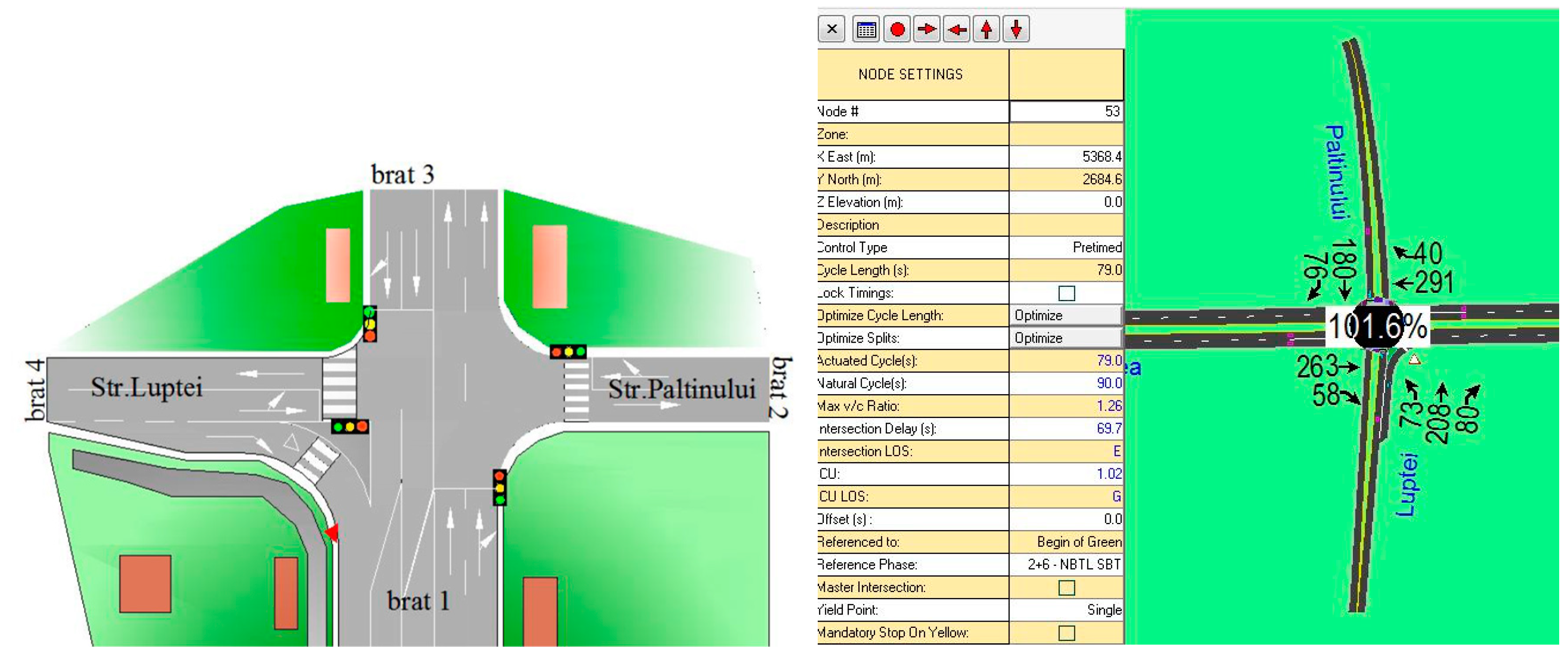
• completing the fields in Synchro Studio 8 modeling software windows with appropriate values [25].

This resulted in a series of data that helped to determine relevant indicators for assessing intersection performance: traffic intensity, peak time factor and intersection service level,

Table 4. Intersection performance.

	Traffic Intensity	Peak Hour Factor	Intersection Level of Service
Intersection 1 Aral-Milea	1378	0.9963	E
Intersection 2—SemaforuluiPaltinului	1157	0.958	E
Intersection 3—SemaforuluiU.Militara	825	0.7265	D
Intersection 4—IBIS	405	0.517	C
Intersection 5—Turismului	843	0.805	D
Intersection 6—Turnisor	892	0.857	E

.

The number of vehicles through each intersection is shown in

Table 5. Average vehicles for the day.

	Average Vehicles for the Day
Intersection 1 Aral-Milea	2173
Intersection 2—Semaforului Paltinului	1247
Intersection 3—Semaforului U.Militara	1649
Intersection 4—IBIS	810
Intersection 5—Turismului	675
Intersection 6—Turnisor	892

.

The intersections considered are shown in Figure 4.

The analysis of the data obtained during the research, as well as the calculations, led to the identification of the critical points from the traffic point of view, such as:

• Number of traffic accidents;
• Vehicle-vehicle and vehicle-pedestrian conflict points;
• High delays at intersection;
• Shaping the queues (number of stationary vehicles) and generating blockages;
• Increasing the service level;
• Big fuel consumption for 100 km; and
• Protection of the environment by assessing the level of pollution.

All these critical points identified lead to a marked decrease in traffic capacity.

Following the study performed at the intersections analyzed in Sibiu and modeled with Synchro Studio 8, (Figure 5) it was found that regardless of the control mode—semaphores, roundabout, the vehicles use common traffic lanes, which lead to the appearance of conflict points.

At the same time, stopping vehicles at intersections long distances before pedestrians, as well as the location of pedestrian crossings very close to the intersection, make it impossible to observe vehicles at the other entrances and oblige drivers to stop in the area of pedestrian crossing, thus generating conflicts and increased accident risk.

Thus, by modeling with Synchro it is noticeable that the obvious decrease in the traffic capacity of an intersection or road sector is due to the following main factors:

• the lane width (lowering the bandwidth from normal to 3.5 m to 2.5 m leads to a 15% decrease in traffic volume);
• the existence of parking facilities within the 50 m distance before the stop line at the entrance to an intersection leads to a decrease of 35% in the case of a single lane and by 20% for two lanes and 65 maneuvers parking per hour;
• the presence of heavy traffic with a weight of 5% leads to a decrease of 6%, and for a weight of 10% to a decrease by 15% of the bandwidth considered.

The pollutants considered in this paper are:

The Pollutants Considered in This Paper Are:	Legislation/Standards
Carbon monoxide	The law that refers to carbon monoxide in Romania is no. 104 of 15 June 2011. The limit value is 10 mg/m3, the limit value for the protection of human health (the maximum daily 8-h mean value)
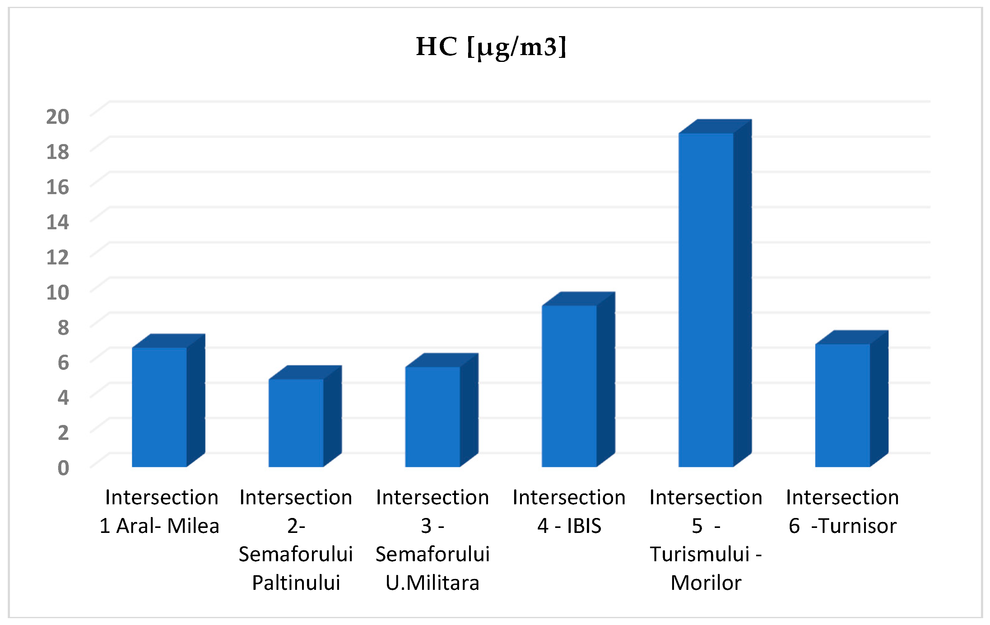
Hydrocarbons (HC)	Low no. 104 of 15 June 2011
NOx	Law no. 278 of 24/10/2013
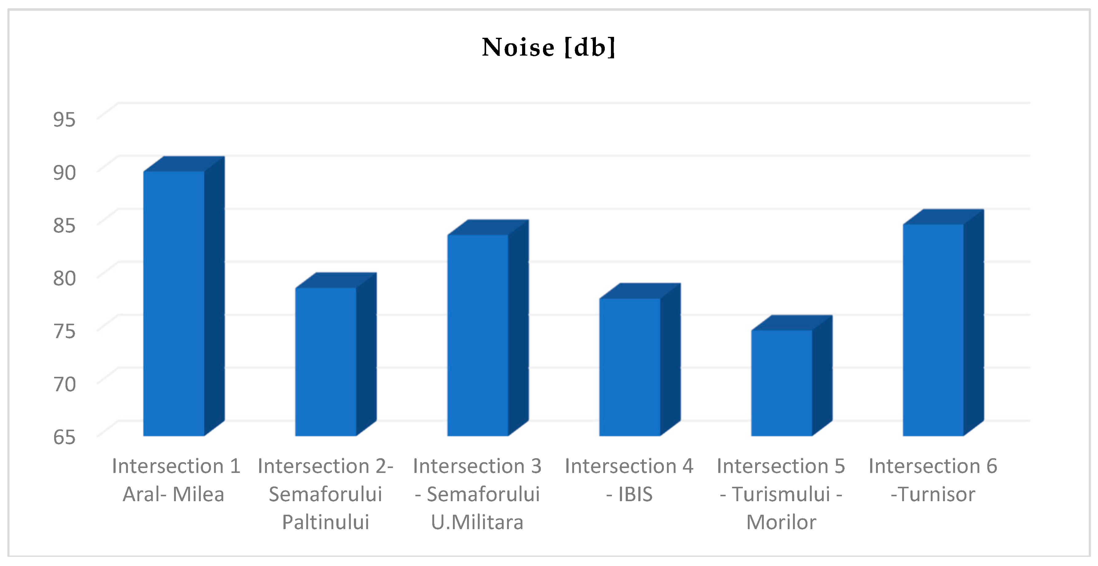
Noise	Order of the Minister of Health 536/1997, STAS 10009-88—Urban Acoustics. Permissible limits of urban noise level.
Ozon	Law no. 278 of 24/10/2013
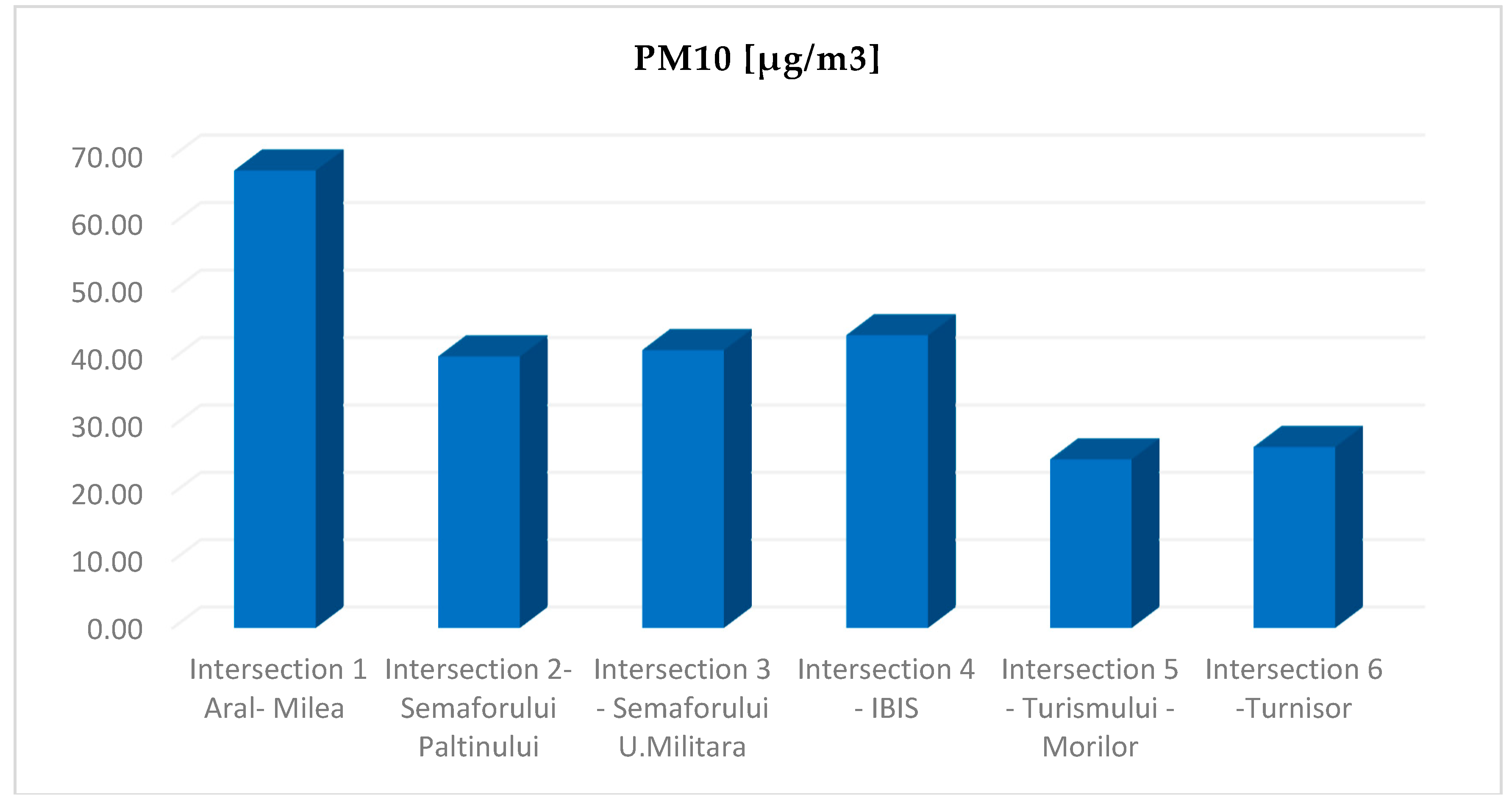
PM10	Law no. 278 of 24/10/2013, Directive 2008/50/EC of the European Parliament and of the Council of the European Union of 21 May 2008

3. Results and Discussions

The pollutants taken into account are presented in

Table 6. Pollutant factors at intersections.

	CO [µg/m3]	HC [µg/m3]	Nox [µg/m3]	Noise [dB]	Ozone Concentration [µg/m3]	PM10 [µg/m3]
Intersection 1 Aral-Milea	187	7	16	91.36	39.14	67.87
Intersection 2 Semaforului Paltinului	170	5	23	80.56	38.22	40.33
Intersection 3 Semaforului-U.Militara	165	6	19	85.3	37.97	41.27
Intersection 4 IBIS	187	10	37	78.1	40.08	43.48
Intersection 5 Turismului-Morilor	245	19	49	76.3	40.33	25.06
Intersection 6 Turnisor	235	7	21	86.32	39.88	26.89

.

The variation of factors taken into account in the analysis is shown in Figure 6.

The importance of each intersection was determined by the average number of cars crossing intersections one day, Figure 7.

In stage 1, as we have shown above, we use the AHP multichannel method to calculate the weight of each factor taken into account.

The Saaty table on the importance of intersections is presented in

Table 7. The Saaty table.

	Intersection 1 Aral-Milea	Intersection 2 Semaforului Paltinului	Intersection 3 Semaforului-U.Militara	Intersection 4 IBIS	Intersection 5 Turismului-Morilor	Intersection 6 Turnisor
Intersection 1 Aral-Milea	1	3	2	4	5	4
Intersection 2 SemaforuluiPaltinului	0.333333333	1	0.5	3	4	3
Intersection 3 Semaforului-U.Militara	0.5	2	1	4	5	4
Intersection 4 IBIS	0.25	0.333333333	0.25	1	2	1
Intersection 5 Turismului-Morilor	0.2	0.25	0.2	0.5	1	0.5
Intersection 6 Turnisor	0.25	0.333333333	0.25	1	2	1

.

Through calculations specific to the AHP method, the percentage of each intersection is calculated. The weight of each intersection according to the average number of cars passing through it is shown in

Table 8. AHP method application.

	Weight Intersections
Intersection 1 Aral-Milea	0.36006879
Intersection 2 Semaforului Paltinului	0.17502927
Intersection 3 Semaforului-U.Militara	0.26339513
Intersection 4 IBIS	0.07663535
Intersection 5 Turismului-Morilor	0.04823611
Intersection 6 Turnisor	0.07663535

.

Carbon monoxide is a toxic gas, with high concentrations being fatal (at concentrations of about 100 mg/m³) by reducing the oxygen transport capacity in the blood, with consequences on the respiratory and cardiovascular system. At relatively low concentrations it:

• affects the central nervous system;
• weakens the heart rate, thus reducing the volume of blood distributed in the body;
• reduces visual acuity and physical capacity;
• short-term exposure may cause acute fatigue;
• can cause breathing difficulties and chest pain in people with cardiovascular disease;
• causes irritability, migraines, rapid breathing, lack of coordination, nausea, dizziness, confusion;
• reduces concentration.

The population segment most affected by carbon monoxide exposure is: children, elderly, people with respiratory and cardiovascular disease, anemic persons, and smokers. The carbon monoxide values are presented in Figure 8.

The Saaty table according to measured CO emissions is shown in

Table 9. Saaty table based on measured CO emissions.

CO	Intersection 1 Aral-Milea	Intersection 2 Semaforului Paltinului	Intersection 3 Semaforului-U.Militara	Intersection 4 IBIS	Intersection 5 Turismului-Morilor	Intersection 6 Turnisor
Intersection 1 Aral-Milea	1	0.5	0.5	1	3	3
Intersection 2 SemaforuluiPaltinului	2	1	1	2	4	4
Intersection 3 Semaforului-U.Militara	2	1	1	2	4	4
Intersection 4 IBIS	1	0.5	0.5	1	3	3
Intersection 5 Turismului-Morilor	0.333333333	0.25	0.25	0.333333333	1	1
Intersection 6 Turnisor	0.333333333	0.25	0.25	0.333333333	1	1

.

Hydrocarbons (HC) are pollutants present in car emissions characterized by varying toxicity depending on the chemical composition. The main hydrocarbons in the exhaust gases of cars are benzene, toluene and xylenes. The HC values measured at intersections are presented in Figure 9.

The Saaty table according to the measured HC emissions is shown in

Table 10. Saaty table based on measured HC values.

HC [µg/m3]	Intersection 1 Aral-Milea	Intersection 2 Semaforului Paltinului	Intersection 3 Semaforului-U.Militara	Intersection 4 IBIS	Intersection 5 Turismului-Morilor	Intersection 6 Turnisor
Intersection 1 Aral-Milea	1	0.5	1	2	4	1
Intersection 2 SemaforuluiPaltinului	2	1	1	3	5	2
Intersection 3 Semaforului-U.Militara	1	1	1	2	3	1
Intersection 4 IBIS	0.5	0.3333	0.5	1	2	0.5
Intersection 5 Turismului-Morilor	0.25	0.2	0.3333	0.5	1	0.333
Intersection 6 Turnisor	1	0.5	1	2	3	1

.

3.1. NOx Nitrogen Oxides

Nitrogen dioxide is known to be a very toxic gas for both humans and animals (the degree of toxicity of nitrogen dioxide is 4 times higher than that of nitrogen monoxide). Exposure to high concentrations can be fatal, and at low concentrations, it affects lung tissue. The population exposed to this type of pollutant may have breathing difficulties, respiratory irritation, lung dysfunctions. Long-term exposure at a low concentration can destroy lung tissue resulting in pulmonary emphysema. People most affected by exposure to this pollutant are children. The NOx values measured at intersections are presented in Figure 10. The Saaty table according to the measured NOx emissions is shown in

Table 11. Saaty table based on measured NOx values.

NOx	Intersection 1 Aral-Milea	Intersection 2 Semaforului Paltinului	Intersection 3 Semaforului-U.Militara	Intersection 4 IBIS	Intersection 5 Turismului-Morilor	Intersection 6 Turnisor
Intersection 1 Aral-Milea	1	2	1	3	4	2
Intersection 2 SemaforuluiPaltinului	0.5	1	1	2	3	1
Intersection 3 Semaforului-U.Militara	1	1	1	2	3	1
Intersection 4 IBIS	0.3333333	0.5	0.5	1	2	0.5
Intersection 5 Turismului-Morilor	0.25	0.3333333	0.3333333	0.5	1	0.3333333
Intersection 6 Turnisor	0.5	1	1	1	3	1

.

3.2. Noise

Noise is defined as a complex of sounds without a periodic character [26], with a random disgusting insurgency that affects the psychological and biological state of humans and other organisms in nature. The physical or objective characteristics of noise refer to strength or sound intensity, duration, and frequency. Intensity is the most important feature that depends on the features of the source, the distance, and the possibilities of transmission or multiplication. It is measured in decibels.

Phono is the physiological unit of perception by the human ear of the weakest sound excitation. It was admitted that the Figure 11 on the scale of decibels, or on the scale of foni AA1, represents the threshold at which the intensity of the sound becomes harmful. Excessive exposure to intense noise over long periods of time causes deafness.

The Saaty table according to the measured noise at intersections is shown in

Table 12. Saaty table based on the measured noise.

Noise	Intersection 1 Aral-Milea	Intersection 2 Semaforului Paltinului	Intersection 3 Semaforului-U.Militara	Intersection 4 IBIS	Intersection 5 Turismului-Morilor	Intersection 6 Turnisor
Intersection 1 Aral-Milea	1	0.25	0.5	0.25	0.2	0.5
Intersection 2 SemaforuluiPaltinului	4	1	2	1	0.5	2
Intersection 3 Semaforului-U.Militara	2	0.5	1	3	0.3333333	1
Intersection 4 IBIS	4	1	2	1	1	2
Intersection 5 Turismului-Morilor	5	2	3	1	1	2
Intersection 6 Turnisor	2	0.5	1	0.5	0.5	1

.

3.3. Ozone

In large quantities, ozone has a negative influence on health. An increase in mortality by 0.66% due to higher ozone concentrations in the summer months is quoted (study in 23 European cities). Moreover, in China a similar study has demonstrated a 0.45% increase in ozone-depleted mortality. The increase in ozone in the environment is followed by a proportional increase of it in homes, schools, hospitals, workplaces and cars with harmful effects [27]. Ozone values measured at intersection are presented in Figure 12.

The Saaty table for ozone concentration measured at intersections is shown in

Table 13. Saaty table based on the measured ozone values.

Ozone	Intersection 1 Aral-Milea	Intersection 2 Semaforului Paltinului	Intersection 3 Semaforului-U.Militara	Intersection 4 IBIS	Intersection 5 Turismului-Morilor	Intersection 6 Turnisor
Intersection 1 Aral-Milea	1	0.5	0.33333	2	3	2
Intersection 2 SemaforuluiPaltinului	2	1	0.5	2	3	2
Intersection 3 Semaforului-U.Militara	3	2	1	3	4	3
Intersection 4 IBIS	0.5	0.5	0.3333333	1	2	1
Intersection 5 Turismului-Morilor	0.3333333	0.3333333	0.25	0.5	1	0.5
Intersection 6 Turnisor	0.5	0.25	0.3333333	1	2	1

.

3.4. Particulate Matter (PM10)

Particulates are among the most dangerous sources of pollution. Suspended particles are a complex mixture of very small particles and liquid droplets [28]. Suspended particulate matter (PM10) comes mainly from pollutant emissions from industry, traffic, and home heating.

These can cause asthma, cardiovascular disease, lung cancer, and premature death. According to Directive 2008/50/EC of the European Parliament and of the Council of the European Union, member states are required to reduce PM2.5 exposure in urban areas by 20% on average by 2020 based on 2010 levels (target value 25 micrograms/m3/day) [29]. Particulate matter (PM10) values measured at intersections are presented in Figure 13.

The Saaty table for susceptible particles, measured at intersections, is shown in

Table 14. Saaty table based on PM10 values measured.

PM10	Intersection 1 Aral-Milea	Intersection 2 Semaforului Paltinului	Intersection 3 Semaforului-U.Militara	Intersection 4 IBIS	Intersection 5 Turismului-Morilor	Intersection 6 Turnisor
Intersection 1 Aral-Milea	1	0.25	0.3333333	0.3333333	0.142857143	0.1666667
Intersection 2 SemaforuluiPaltinului	4	1	2	3	0.3333333	0.5
Intersection 3 Semaforului-U.Militara	3	0.5	1	2	0.25	0.3333333
Intersection 4 IBIS	2	0.3333333	0.5	1	0.2	0.25
Intersection 5 Turismului-Morilor	7	3	4	5	1	2
Intersection 6 Turnisor	6	2	3	4	0.5	1

.

The weights of all pollutants in each intersection are shown in

Table 15. The weights of all pollutant factors.

	CO	HC	Nox	Noise	Ozon Concentration	PM10
Intersection 1 Aral-Milea	0.160119048	0.184407669	0.289578346	0.05137842	0.164619883	0.036097917
Intersection 2 SemaforuluiPaltinului	0.278571429	0.290681785	0.181219149	0.191362738	0.215629984	0.189769821
Intersection 3 Semaforului-U.Militara	0.278571429	0.198733315	0.204474963	0.161340582	0.351222754	0.117817562
Intersection 4 IBIS	0.160119048	0.096134652	0.099693877	0.214947644	0.107057416	0.068218244
Intersection 5 Turismului-Morilor	0.061309524	0.054894169	0.061358375	0.273496794	0.063503456	0.403665814
Intersection 6 Turnisor	0.061309524	0.17514841	0.163675289	0.107473822	0.097966507	0.290537084

.

Variation of pollutants according to their weight is shown in Figure 14.

We calculate the proportion of pollutants according to the importance of intersections (no cars),

Table 16. Weight of pollutants.

Pollutant Name	Weight
CO	0.18084854
HC	0.238524318
NOx	0.227281735
NOISE	0.127603682
OZONE	0.102802982
PM10	0.131070247

. Variation of weights for each pollutant is shown in Figure 15.

These weights will be used as entry data in the second stage of the TOPSIS method.

	CO [µg/m3]	HC [µg/m3]	NOx [µg/m3]	Noise [dB]	Ozone Concentration[µg/m3]	PM10 [µg/m3]
Weight	0.18084	0.23852	0.22728	0.1276036	0.102803	0.13107
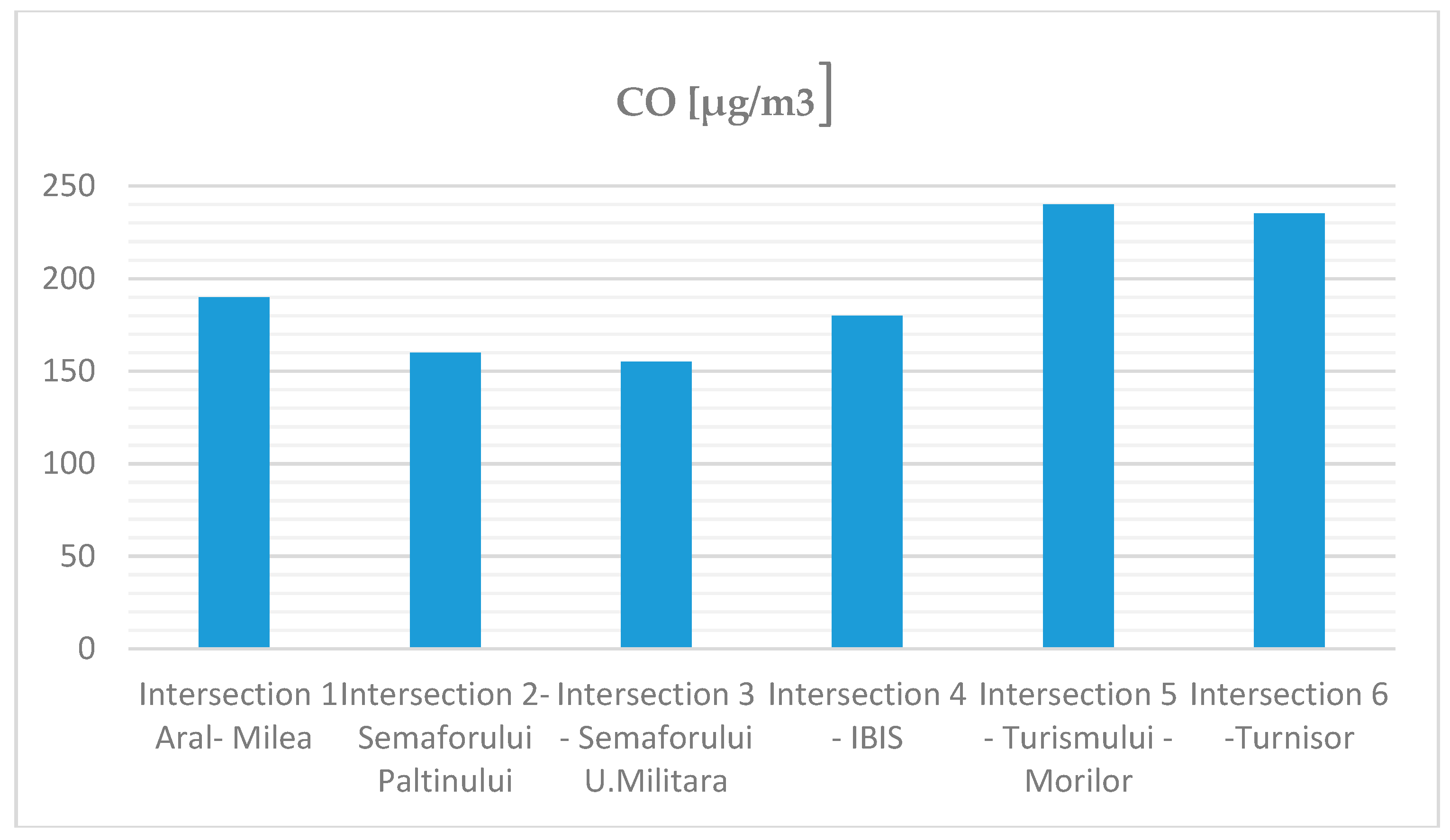
Intersection 1 Aral-Milea	187	7	16	91.36	39.14	67.87
Inter SemaforuluiPaltinului	170	5	23	80.56	38.22	40.33
Intersection 3 Semaforului-U.Militara	165	6	19	85.3	37.97	41.27
Intersection 4 IBIS	187	10	37	78.1	40.08	43.48
Intersection 5 Turismului-Morilor	245	19	49	76.3	40.33	25.06
Intersection 6 Turnisor	235	7	21	86.32	39.88	26.89

Sum of squares of each column

241,313

620

5357

41,485.0956

9257.7586

11,177.64

Matrix V
Intersection 1 Aral-Milea	0.068844025	0.067056	0.049685	0.057236524	0.041818997	0.084141
Intersection 2 SemaforuluiPaltinului	0.062585477	0.047897	0.071422	0.050470385	0.040836026	0.049999
Intersection 3 Semaforului-U.Militara	0.060744728	0.057476	0.059001	0.053439968	0.040568914	0.051164
Intersection 4 IBIS	0.068844025	0.095794	0.114896	0.048929209	0.042823336	0.053904
Intersection 5 Turismului-Morilor	0.090196717	0.182008	0.15216	0.047801519	0.043090448	0.031068
Intersection 6 Turnisor	0.086515219	0.067056	0.065211	0.054078992	0.042609647	0.033336
A+	0.060744728	0.047897	0.049685	0.047801519	0.040568914	0.031068
A−	0.090196717	0.182008	0.15216	0.057236524	0.043090448	0.084141

Positive Ideal Solution
Intersection 1 Aral-Milea	6.55986E-05	3.67E-04	0	8.90193E-05	1.56271E-06	2.8172E-03
Intersection 2 SemaforuluiPaltinului	3.38836E-06	0	4.7E-4	7.12285E-06	7.13486E-08	3.58E-04
Intersection 3 Semaforului-U.Militara	0	9.18E-05	8.68E-05	3.17921E-05	0	4.04E-04
Intersection 4 IBIS	6.55986E-05	2.2942E-03	4.253E-03	1.27168E-06	5.08242E-06	5.21E-04
Intersection 5 Turismului-Morilor	8.67428E-04	1.79861E-02	1.05011E-02	0	6.35813E-06	0
Intersection 6 Turnisor	6.641186E-04	3.673E-04	2.4112E-04	3.94067E-05	4.16459E-06	5.15E-06

Intersection 1 Aral-Milea	0.057792632
Intersection 2 SemaforuluiPaltinului	0.029007895
Intersection 3 Semaforului-U.Militara	0.024782979
Intersection 4 IBIS	0.08449885
Intersection 5 Turismului-Morilor	0.171349608
Intersection 6 Turnisor	0.036345096

Negative Ideal Solution
Intersection 1 Aral-Milea	4.559374E-04	1.32141E-02	1.105011E-02	0	1.61659E-06	0
Intersection 2 SemaforuluiPaltinului	7.6238E-04	1.798E-02	6.519E-03	4.57806E-05	5.08242E-06	1.166E-03
Intersection 3 Semaforului-U.Militara	8.6712E-04	1.5508E-02	8.679E-03	1.44138E-05	6.35813E-06	1.087E-03
Intersection 4 IBIS	4.5593E-04	7.433E-03	1.389E-03	6.90115E-05	7.13486E-08	9.14E-04
Intersection 5 Turismului-Morilor	0	0	0	8.90193E-05	0	2.817E-03
Intersection 6 Turnisor	1.35534E-05	1.3214E-02	7.56E-03	9.97001E-06	2.3117E-07	2.5812E-03

Intersection 1 Aral-Milea	0.155475792
Intersection 2 SemaforuluiPaltinului	0.162737014
Intersection 3 Semaforului-U.Militara	0.161748073
Intersection 4 IBIS	0.101295549
Intersection 5 Turismului-Morilor	0.053905193
Intersection 6 Turnisor	0.152901674

The ranking of intersections according to the TOPSIS multicriteria method [30], from the pollution point of view, in the order of the smallest polluted to the most polluted area, considering the pollutants measured at each intersection, is presented in

Table 17. The ranking of intersections according to the TOPSIS multicriteria method.

Intersection Name	Value of TOPSIS	RANK
Intersection 5 Turismului-Morilor	0.239307633	1
Intersection 4—IBIS	0.545202384	2
Intersection 1 Aral-Milea	0.729014588	3
Intersection 6 Turnisor	0.807948659	4
Intersection 2 Semaforului-Paltinului	0.848716217	5
Intersection 3 Semaforului-U.Militara	0.867137517	6

.

Unfortunately, present-day economics does not provide the conceptual framework needed to build such an economy. It will have to be designed with an understanding of basic ecological concepts such as sustainable yield, carrying capacity, nutrient cycles, the hydrological cycle, and the climate system.

Economic activity is permanently accompanied by negative unwanted factors, such as unemployment, and more recently intensely analyzed, pollution. Since 1991 the environmental Kuznets curve (EKC) has become a standard feature in the technical literature of environmental policy, [31] and as it is challenged, we are not removing the negative external effects that economic development is causing to the planet’s inhabitants and the environment.

Sustainable development also involves an external cost. This cost we are trying to analyze in this paper needs to be reduced to keep it within acceptable limits and sustained so as not to threaten the sustainable development process. This is why the threat is increasingly alarming and even if it has been discussed globally for some time, it is becoming increasingly serious with adverse effects for humanity such as the threat of climate change, the disappearance of some species of plants and animals, a widening of the hole in the ozone layer, and the list could continue.

The international community has decided to deal with environmental issues through global collective action, which it has sought to define and apply through an appropriate international framework. This international framework of action has been built over time and is in a dynamic evolution, encompassing binding legal measures in the form of treaties or conventions or non-binding in the form of declarations, resolutions or sets of guidelines and policy orientations, institutional measures and viable funding mechanisms, and the Declaration of the United Nations Conference on the Human Environment.

The United Nations Conference on Human Environment, 5–16 June 1972, met in Stockholm and considered the need for a common outlook and common principles to inspire and guide the world’s people in preserving and enhancing the human environment. They proclaimed the Declaration of the United Nations Conference on Human Environment, and there are some important points related to this that are connected our study:

For example: The protection and improvement of the human environment is a major issue which affects the well-being of peoples and economic development throughout the world; it is the urgent desire of the peoples of the whole world and the duty of all governments. Local and national governments will bear the greatest burden of large-scale environmental policy and action within their jurisdictions. International cooperation is also needed in order to increase resources to support developing countries in carrying out their responsibilities in this field. A growing class of environmental problems, because they are regional or global in extent or because they affect the common international realm, will require extensive cooperation among nations and action by international organizations in the common interest.

The Conference calls upon governments and peoples to exert common efforts for the preservation and improvement of the human environment, for the benefit of all the people and for their posterity. In principle 18 is proclaimed that: science and technology, as part of their contribution to economic and social development, must be applied to the identification, avoidance and control of environmental risks, the solution of environmental problems, and for the common good of mankind, [32].

If we look at the statistical data, there is obvious evidence that the world’s poor countries exert the slightest pressure on the planet’s balance. They are limited polluters and this is also due to low levels of economic development. It is therefore a reality that the greenhouse effect and the warming of the Earth is not primarily due to poor countries. The present study is conducted in a developed economy and it is observed that in contradictory ways these studies and the attention given to the environment are underway. However, in a contradictory way, care and respect for everything environmental seems to be an attitude embraced by economically developed countries.

When we talk about the eco-economy, we cannot not discuss without connecting it with the bio-economy, and then rediscover the Romanian economist Georgescu-Roegen. More and more papers contain this element of the bio-economy because we cannot discuss sustainable development without quoting Georgescu-Roegen.

Roegen’s suggestions have prompted and still prompted a lively and real interest. Evidence is also that there is no serious work on sustainable development without reference to its original analysis. Even when proposing concrete plans to combat pollution, the authors do not forget that they remain in line with the entropy of roegenian origin. Consumption for the sake of fashion, such as the production of a new machine every year must be considered bioeconomic crime; we must focus on sustainability, designing products for a long life and easy repairs [33].

Classical and neo-classical economic theory has made its monetary economic calculation a support for its rigor and modernity. Attempts from the East to bring reality by replacing monetary terms with physical analysis have, in the final analysis, been ridiculed. Relative to such an unsuccessful experience, there is no reason to renounce a gained asset. At the same time, those concerned with the problems of sustainable development find that there are certain difficulties related precisely to the way in which the environmental elements of value are valued [34].

The inclination to quality “and not to quantity”, to use a preferred expression by Keynes, becomes an imperative because, as Paul Bran warned, The Entropy Value Act will not forgive us if we do not urgently nourish Nature with services to reduce pollution and to repair what we have corrupted in the years of “industrial unleashing”, the theft of low entropy, theft accompanied, in many cases, by environmental crime [35].

4. Conclusions

As a result of the aforementioned emissions of pollutants resulting from traffic, CO₂ has the highest share. For reducing polluting emissions in the atmosphere durable transport needs to be developed.

This can be achieved by:

• Use of fuels with a lower lead content;
• The progressive diminution of the park of highly polluting means of transport;
• Streamlining road traffic at crowded intersections (through the green traffic light, setting unique rolling paths);
• The elaboration and approval of the concept of greening the land near the traffic arteries and the creation of protection screens from the vegetation between the streets and the living spaces;
• Eco-economy was a large multi-element system, and exchanges of material, energy and information existed among various subsystems of the large system. Owing to system complexity, selecting proper factors as far as possible to establish a comprehensive index system was important to eco-economy assessment. According to the representative features of regional eco-environment problems in Sibiu city, including natural conditions, environmental pollution and social economic aspects must be considered. Based on the results, natural environment and human economic activities were the most significant factors affecting eco-economy quality. Nevertheless, pollution was also regarded as sensitive factors to decide the regional eco-economy quality in some particular areas;
• Economic development, the problem of pollution, and the correlation between them and socio-economic variables has lately gained more and more attention among a growing number of ecologists, sociologists, philosophers and increasingly economists. After presenting and analyzing for this paper some of previous research, with some of them quoted here, in this area of pollution transportation and eco-economy, we can further illustrate and conclude the reach of countries that have the most devastating impact on the environment. In those countries and especially in the most developed cities, this model of measurement of pollution in intersection can be applied;
• This research could be applied to other cities for the integrated assessment of ecological environment.

The advantages of using multi-criteria methods are:

• The use of the two AHP and TOPSIS multi-criteria methods allowed an accurate analysis of the intersections in Sibiu for air pollution, noise, and traffic. Although the AHP methods decompose the main problem into a number of subsystems and allow a relatively large number of comparisons, this is not a disadvantage, because the results that we can offer along with the other multicriteria method represent a significant advantage in determining the decisions that should be taken for the health of humans.
• The two methods allow you to connect to different domains from the initial problem. Taking into account the issue of urban traffic, important conclusions can be drawn impacting on the eco-economy.
• Another advantage is that the study can be applied to other areas around the world. In spite of the cost in terms of the measurements made for this analysis, they should not be considered expensive because they are focused on a solution through eco-economy that may reduce disease and save lives.
• Although in the literature the limited number of criteria can be considered a disadvantage of the AHP method, in the context of the study that we conducted in this paper it has not raised any problems, with the nine criteria being sufficient for the evaluation of the multiple factors considered and for the conclusion.

References

- Brown, L.R. The Economy and the Earth: The Option: Restructure or Decline. In Eco-Economy: Building an Economy for the Earth; Earth Policy Institute: Washington, DC, USA, 2001; Chapter 1. [Google Scholar]
- Playtech. Available online: https://playtech.ro/2018/pollution-mortality-deaths-2015 (accessed on 18 June 2018).
- Sinem, D.; Ferhat, B.; Sait, C.S. MCDM analysis of wind energy in Turkey: Decision making based on environmental impact. Environ. Sci. Pollut. Res. 2018, 25, 19753–19766. [Google Scholar]
- Ramanathan, R. A note on the use of the analytic hierarchy process for environmental impact assessment. J. Environ. Manag. 2001, 63, 27–35. [Google Scholar] [CrossRef] [PubMed]
- Tolga, K.; Kahraman, C. An integrated fuzzy AHP–ELECTRE methodology for environmental impact assessment. Expert Syst. Appl. 2011, 38, 8553–8562. [Google Scholar] [CrossRef]
- Ren, J.; Liang, H. Multi-criteria group decision-making based sustainability measurement of wastewater treatment processes. Environ. Impact Assess. Rev. 2017, 65, 91–99. [Google Scholar] [CrossRef]
- Ouyang, X.; Guo, F. Intuitionistic fuzzy analytical hierarchical processes for selecting the paradigms of mangroves in municipal wastewater treatment. Chemosphere 2018, 197, 634–642. [Google Scholar] [CrossRef] [PubMed]
- Air Quality Framework Directive 96/62/ECof the European Parliament and the Council. Available online: http://ec.europa.eu/environment/air/quality/index.htm (accessed on 9 July 2018).
- Beria, P.; Maltese, I.; Mariotti, I. Comparing Cost Benefit and Multi-Criteria Analysis: The Evaluation of Neighbourhoods Sustainable Mobility. Available online: http://ww2.unime.it/sefisast/SEFISAST/Conference_Paper_files/BERIA_MALTESE_MARIOTTI.pdf (accessed on 19 August 2018).
- Wang, J.J.; Jing, Y.-Y.; Zhang, C.-F.; Zhao, J.-H. Review on multi-criteria decision analysis aid in sustainable energy decision-making. Renew. Sustain. Energy Rev. 2009, 13, 2263–2278. [Google Scholar] [CrossRef]
- Misra, S.K.; Ray, A. Comparative study on different multi-criteria decision making tools in software project selection scenario. Int. J. Adv. Res. Comput. Sci. 2012, 3. [Google Scholar] [CrossRef]
- Caterino, N.; Iervolino, I.; Manfredi, G.; Cosenza, E. Applicability and effectivenessof different decision making methods for seismic upgrading building structures. In Proceedings of the XIII Convegno Nazionale L’Ingegneria Sismica, Bologna, Italy, 28 June–2 July 2009. [Google Scholar]
- Wang, M.; Liu, S.; Wang, S.; Lai, K.K. A weighted product method for bidding strategies in multi-attribute auctions. J. Syst. Sci. Complex. 2010, 23, 194–208. [Google Scholar] [CrossRef]
- Chang, Y.H.; Yeh, C.H. Evaluating airline competitiveness using multiattribute decision making. Omega 2001, 29, 405–415. [Google Scholar] [CrossRef]
- Saaty, T.L. The Analytic Network Process; RWS Publications: Pittsburgh, PA, USA, 2001. [Google Scholar]
- Saaty, T.L. What is the Analytic Hierarchy Process? In Mathematical Models for Decision Support; NATO ASI Series; Springer: Berlin/Heidelberg, Germany, 1988; Volume 48, pp. 109–121. [Google Scholar]
- Govindan, K.; Jepsen, M.B. ELECTRE: A comprehensive literature review on methodologies and applications. Eur. J. Oper. Res. 2016, 250, 1–29. [Google Scholar] [CrossRef]
- Buchanan, J.; Sheppard, P.; Vanderpoorten, D. Ranking projects using the ELECTRE method. In Proceedings of the 33rd Annual Conference in Operational Research Society of New Zeeland, Auckland, New Zealand, 30 August–2 September 1998; pp. 42–51. [Google Scholar]
- Hwang, C.L.; Yoon, K. Multiple Attribute Decision Making: Methods and Applications; Springer: New York, NY, USA, 1981. [Google Scholar]
- Boran, F.E.; Genç, S.; Kurt, M.; Akay, D. A multi-criteria intuitionistic fuzzy group decision making for supplier selection with TOPSIS method. Expert Syst. Appl. 2009, 36, 11363–11368. [Google Scholar] [CrossRef]
- Highway Capacity Manual; National Research Council: Ottawa, ON, Canada, 2000; ISBN 0-309-06681-6. Available online: https://sjnavarro.files.wordpress.com/2008/08/highway_capacital_manual.pdf (accessed on 04 September 2018).
- Kijawattanee, U.; Teeratat, A.; Sorawee, W.; Patrachart, K.; Rudjanakanoknad, A.; Chaodit, A. Traffic Data Analysis on Sathorn Road with Synchro Optimization and Traffic Simulation. Eng. J. 2017, 21, 57–67. [Google Scholar] [CrossRef] [Green Version]
- FLOREA, D. ş.a. Managementul traficului rutier; Editura Universităţii “Transilvania din Braşov”: Brașov, Romania, 1998; ISBN 973-98-512-7-43. [Google Scholar]
- FLOREA, D. Sisteme Avansate de Transport Rutier; Editura Universităţii “Transilvania” din Braşov: Brașov, Romania, 2006; ISBN 10-973-635-775-9. [Google Scholar]
- Rajakumara, H.N.; Gowda, R.M.M. Road traffic noise prediction models: A Review. Int. J. Sustain. Dev. Plan. 2008, 3. [Google Scholar] [CrossRef]
- Wikipedia. Available online: https://ro.wikipedia.org/wiki/Poluare_acustic%C4%83 (accessed on 05 September 2018).
- Ziarul Lumina. Available online: http://ziarullumina.ro/ozonul-gazul-cu-doua-fete-40107.html (accessed on 6 September 2018).
- CalitateAer. Available online: http://www.calitateaer.ro/public/assessment-page/pollutants-page/pulbere-suspensie-age/?__locale=ro (accessed on 6 September 2018).
- Dr Office. Available online: http://www.systemlife.ro/pm.php (accessed on 6 September 2018).
- Shih, H.-S.; Shyur, H.-J.; Lee, E.S. An extension of TOPSIS for group decision making. Math. Comput. Model. 2007, 45, 801–813. [Google Scholar] [CrossRef]
- Yandle, B.; Vijayaraghavan, M.; Bhattarai, M. The Environmental Kuznets Curve: A Primer; PERC Research Study 02-1; Property and Environment Research Center: Bozeman, Montana, USA, 2002; Available online: https://www.perc.org/articles/environmental-kuznets-curve (accessed on 7 September 2018).
- UN Documents Gathering a Body of Global Agreements. Available online: http://www.un-documents.net/unchedec.htm (accessed on 7 September 2018).
- Georgescu, N.R. Man and Opera; Expert Publishing House: Bucharest, Romania, 1996; Volume 1, pp. 257–263. [Google Scholar]
- Pohoata, I. Strategii si Politici Europene de Dezvoltare Durabila, Suport Curs. Available online: http://www.cse.uaic.ro/_fisiere/Documentare/Suporturi_curs/II_Strategii_si_politici_europene_de_dezvoltare_durabila.pdf (accessed on 8 September 2018).
- Bran, P. Value Economics; Science Publishing House: Chisinau, Moldova, 1991; p. 87. [Google Scholar]