Seasonal Urban Carbon Emission Estimation Using Spatial Micro Big Data


1
Center for Global Environmental Research, National Institute for Environmental Studies, 16-2 Onogawa, Tsukuba, Ibaraki 305-8506, Japan
2
Department of Statistical Data Science, The Institute of Statistical Mathematics, 10-3 Midori-cho, Tachikawa, Tokyo 190-8562, Japan
3
Center for Spatial Information Science, The University of Tokyo, 5-1-5 Kashiwanoha, Kashiwa, Chiba 277-8568, Japan
*
Author to whom correspondence should be addressed.
Sustainability 2018, 10(12), 4472; https://doi.org/10.3390/su10124472
Submission received: 15 September 2018
/
Revised: 22 November 2018
/
Accepted: 23 November 2018
/
Published: 28 November 2018
(This article belongs to the Special Issue Spatial Analysis of Urbanization towards Urban Sustainability)
Abstract
:The objective of this study is to map direct and indirect seasonal urban carbon emissions using spatial micro Big Data, regarding building and transportation energy-use activities in Sumida, Tokyo. Building emissions were estimated by considering the number of stories, composition of use (e.g., residence and retail), and other factors associated with individual buildings. Transportation emissions were estimated through dynamic transportation behaviour modelling, which was obtained using person-trip surveys. Spatial seasonal emissions were evaluated and visualized using three-dimensional (3D) mapping. The results suggest the usefulness of spatial micro Big Data for seasonal urban carbon emission mapping; a process which combines both the building and transportation sectors for the first time with 3D mapping, to detect emission hot spots and to support community-level carbon management in the future.
1. Introduction
Low carbon urban/regional management has attracted considerable attention from stakeholders regarding urban sustainability, especially after the Paris Agreement was adopted in December 2015. To date, 228 cities have pledged that by 2020 they will have reduced carbon dioxide emissions (carbon emissions, hereafter) by a combined total of 454 giga-tons/year [1].
Carbon emissions management is an important issue not only in a top-down manner (e.g., emissions regularization by government), but also as a bottom-up approach that each local municipality can use to promote low carbonization on its own [2]. For this, carbon mapping is an effective approach for encouraging/supporting effective carbon management by policy makers [3]. Carbon mapping allows us to compare the relative influences of each emission source (e.g., residences, offices, vehicles), make effective policies, quantify the impact of these policies, and identify hot spots and unexpected emissions—e.g., due to congestion—in a near real-time manner [1]. Further, carbon mapping is useful in avoiding greenwashing, a term used to describe deceptive claims about the environmental benefits of a product, service, or technology, which often inhibit cities from enacting real, sustainable measures.
Because cities have thousands or millions of emission sources, including residences, shops, restaurants, and vehicles, the acquisition of micro geodata is a fundamental component of accurate and high-resolution carbon mapping [4,5]. Fortunately, in recent years, data from individual buildings and vehicle movements has become increasingly easier to obtain, owing to the development of the Internet of Things and sensor technologies [6,7]. These data allow for monitoring building conditions, human movements, market transactions, and many other activities in cities that will offer new and useful insights [8,9,10]. However, the use of these data for carbon monitoring is still quite limited [1,11,12]. It is increasingly important to clarify to what extent micro geodata helps in the visualizing and reduction of carbon, concerning sustainable urban development [13,14,15].
2. Approach to Carbon Mapping
Our study attempts to estimate and visualize the carbon emissions of individual buildings and road links, through a data-driven three-dimensional (3D) carbon mapping approach. According to the existing literature, the main advantages of 3D visualization is to render the shape of complex objects through the integration of dimensions [16,17], to provide public audiences with a more familiar form of illustration [18,19,20], to show absolute or relative object heights [21,22], and to provide a fruitful approach for examining human activity patterns in a dynamic and interactive space–time orientated environment [23]. The target area was Sumida ward, Tokyo (see Figure 1). Sumida ward includes a major commercial district called Kinshi-cho; a redevelopment area around SkyTree, which is a 634 m high tower; and the rest of the area is mainly downtown residential. Note that our objective is not the development of a new 3D mapping method. Rather, we aim to study to what extent spatial Big Data are useful with regards to carbon mapping/monitoring/management. This understanding would be an important first step towards smart carbon management.
2.1. Model
We used a bottom-up approach, which multiplies the number of emission sources with emission factors (i.e., emissions per unit) [24]. Specifically, we used the following model to estimate the building emissions from i-th building in t-th time period, measured in 30 min intervals, with the p-th purpose of use:
where is the total building emissions in Sumida ward with p-th purpose, which is given by [the total emissions with p-th purpose in Japan, ] × [the population share of Sumida ward in Japan] (see Section 2.3). is the total floor area (TFA) used for the p-th purpose in i-th building, and represents the per area emissions. Equation (1) proportionally distributes building emissions in accordance with the weight, , which quantifies the relative magnitude of emissions. For data sources, see the next sub-section.
Likewise, the transportation/car emissions at i-th road link in t-th time period were estimated using the following model:
where is the total car emissions in Sumida ward, given by [the total emissions from cars in Japan, ] × [the population share of Sumida ward]. Equation (2) proportionally distributes the car emissions in proportion to the traffic volume at the i-th road link in t-th time period, . Unlike Equation (1) that assumes different emission intensities by building use, Equation (2) assumes the same emission intensity across vehicles. This assumption was needed because it was difficult to classify global positioning system (GPS) points, which were used to evaluate car volume, into passenger vehicle, freight vehicle, and so on. The estimation of vehicle types from GPS points would be an interesting topic of research in the future.
Emissions are split between direct and indirect emissions. Direct emissions refer to on-site emissions from individuals, buildings, or vehicles, resulting from urban activities. Indirect emissions occur not on-site but at power plants during energy production. For example, indirect emissions on roads are attributable to gasoline production for gasoline vehicles, or electricity production for electric or hybrid vehicles.
This study attempts to estimate these two emissions by disaggregating the total direct and indirect emissions in the Sumida ward, ( and ), which we will introduce in Section 2.2. Section 2.3 and Section 2.4 respectively explain the unit emission and the intensity that are used to define the weights and for the disaggregation. Finally, Section 2.5 explains how to visualize the carbons estimated by substituting these variables into Equations (1) and (2).
2.2. The Total Emissions ( and )
While the above discussed how unit intensities were used to describe the “relative” change of building and transportation emissions, the absolute emission amounts were constrained to the 2016 estimates provided by the Greenhouse Gas Inventory Office (GIO) of Japan, National Institute for Environmental Studies [25]. Specifically, the total direct emissions in Sumida ward were evaluated by [the GIO direct estimate across Japan] × [0.00203 = (population in Sumida ward)/(population in Japan); sources: Census 2015 (Statistics Bureau, Ministry of Internal Affairs and Communications, Japan [26])]. Indirect emissions were also estimated in the same way. Hence, direct emissions were defined as emissions that accompany activities such as energy conversion, production, and transportation, the values of which are allocated to emission sites. On the other hand, indirect emissions were defined as values allocated to users (the end demand category) and manufactured goods according to their respective energy consumption.
The estimated total emissions, which were used as and , are summarized in Table 1. The building emissions were dominated by indirect emissions, whereas transportation emissions were dominated by direct emissions. Based on this result, mapping both types of emissions was required to understand the underlying emission patterns appropriately.
2.3. The Unit Emissions ()
To evaluate the intensity of emissions from individual buildings in Equation (1), we used a report provided by the Japan Institute of Energy [27]. This report summarizes typical hourly energy consumption per TFA in each month for residences, offices, retail, hotels, and hospitals. We used the typical hourly consumption as the basic unit . In other words, we assume that the amount of emissions is proportional to the energy consumption.
Annual emissions per floor area of 1 m2 (i.e., ) are summarized in Table 2. This table clearly shows the difference between residential and non-residential sectors.
Figure 2 plots the relative monthly changes in the energy consumption (i.e., normalized ). Residential energy consumption was lowest late at night and highest in the evening, probably because of cooking, heating, cooling, and so on. Consumption patterns in the office, retail, and hospital sectors were similar; emissions were the highest in August as a result of cooling demand, while they were low in winter. It is also conceivable that the peak in summer is daytime, and at around 09:00 in winter. By contrast, emissions from hotels tended to increase in the afternoon. Emissions from sports facilities had relatively flat patterns in daytime across the summer months from June to September, due to air conditioners being in continuous operation. To better estimate building carbon emissions accurately, consideration must be given to these emission patterns.
Because these data are relatively old, from 2008, we used the data only to evaluate the relative temporal change in emissions. For the absolute amount of emissions, we used statistical data from 2015, which will be explained in the next sub-section.
2.4. The Micro Intensities ( and )
To use the basic unit for carbon mapping, we needed to know the TFA by purpose of use (residential, office, retail, hospital, hotel, and sports) in each building. Fortunately, Zenrin Co. Ltd. (Kitakyushu, Fukuoka, Japan)’s Building Point Data 2013 includes this information [28]. We applied the TFAs in the dataset for , which is in Equation (1).
Note that this data does not include information about building shape. For clear carbon mapping, we used Z-Map TOWN II of Zenrin Co. Ltd., which was provided by the Center for Spatial Information Science, University of Tokyo.
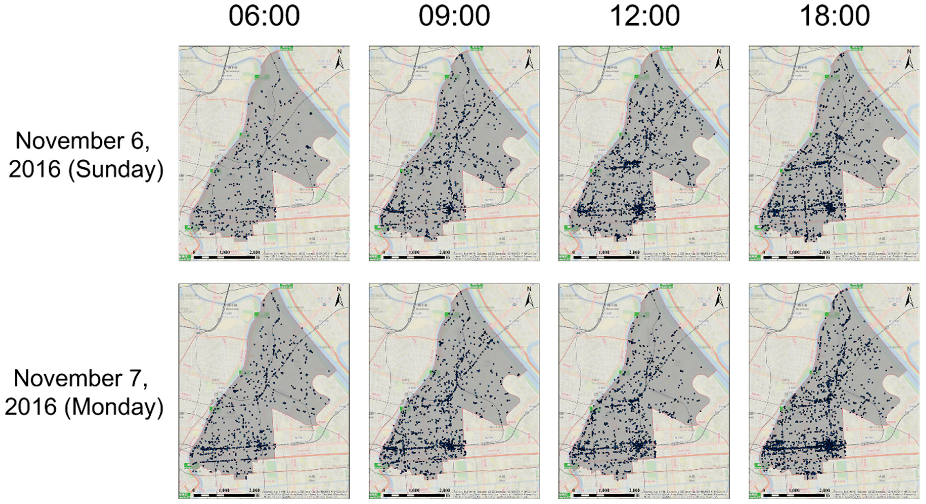
Regarding the intensity of on-road emissions (see Equation (2)), we used the mobile GPS data from 2016 provided by Agoop Coop. (Shibuya, Tokyo, Japan) [29]. This data tracks the location of a specific smartphone application’s users on Android at 30 min intervals, or at 500m intervals on iOS. As an example, Figure 3 plots the GPS points at 08:00, 14:00, and 20:00 for November 6 and 7. The figure shows the ability of this data to capture micro-scale transportation behaviour that changes from day to day. On November 7 (a weekday) the highest activity counts occurred at 08:00 and 20:00, whereas activity peaked at 14:00 on November 6 (a holiday/weekend). Consideration of these differences is important when measuring the daily fluctuation of transportation emissions.
Unfortunately, the GPS data have no information on mode of transportation (i.e., walk, train, or car). To estimate the emissions from vehicles, we needed to identify which GPS points represented vehicles. To achieve this, we assumed that the movement between two GPS points satisfying the following requirements were vehicles: (i) the average speed between two points was more than 6 km/h; and (ii) either or both of these points were more than 50 m away from the railway. Figure 4 plots the GPS points classified as walk (C, green points), train (D, blue points), and vehicle (E, red points) on November 7 using OpenStreetMap (A and B). The points associated with vehicles (Figure 4E) are distributed along major roads. This result is intuitively reasonable. The points assigned to walk (Figure 4D) are concentrated around railways and around Kinshi-cho, a central commercial area containing many pedestrians. These results confirm that we accurately separated GPS points representing cars from those representing train users or pedestrians.
This study focused only on vehicle trips because their emissions are dominant. We defined by the number of vehicles that passed through i-th road link within each 30-min interval indexed by t.
2.5. Mapping Method
Direct and indirect emissions from individual buildings and road links for each month and hour were estimated by substituting the variables explained in Section 2.2, Section 2.3 and Section 2.4 into the model presented in Section 2.1. Estimation results were visualized using ArcScene 10.5, which is a plugin for ArcGIS 10.5 provided by Environmental Systems Research Institute, Inc. (Redlands, California, United States) [30], used for mapping. For easier understanding of carbon emissions on each road and in each building, we displayed temporal (seasonally and hourly) changes in a 3D manner. All tests were conducted for an average weekday in a typical month for each of the four seasons in 2016.
3. Results
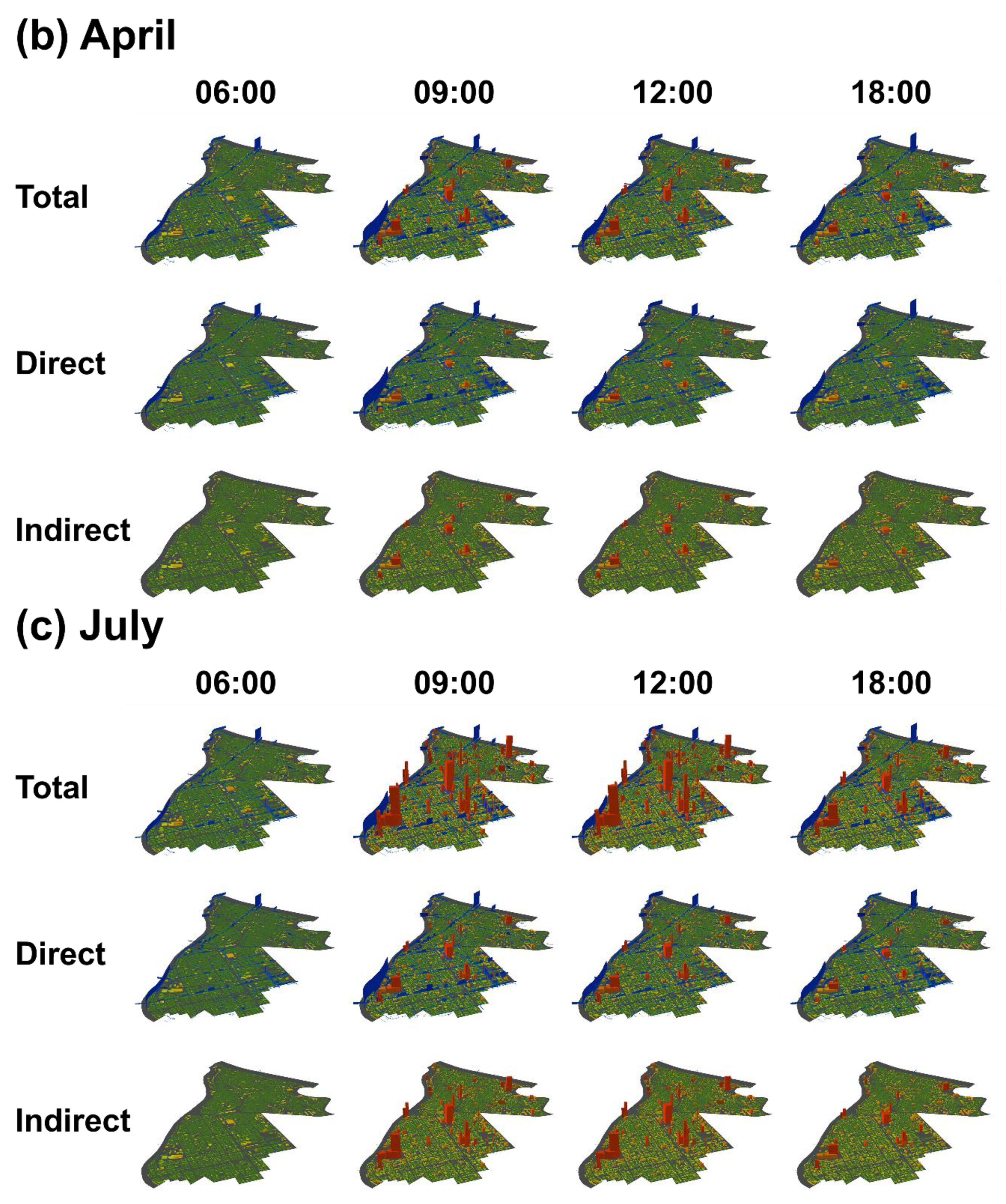
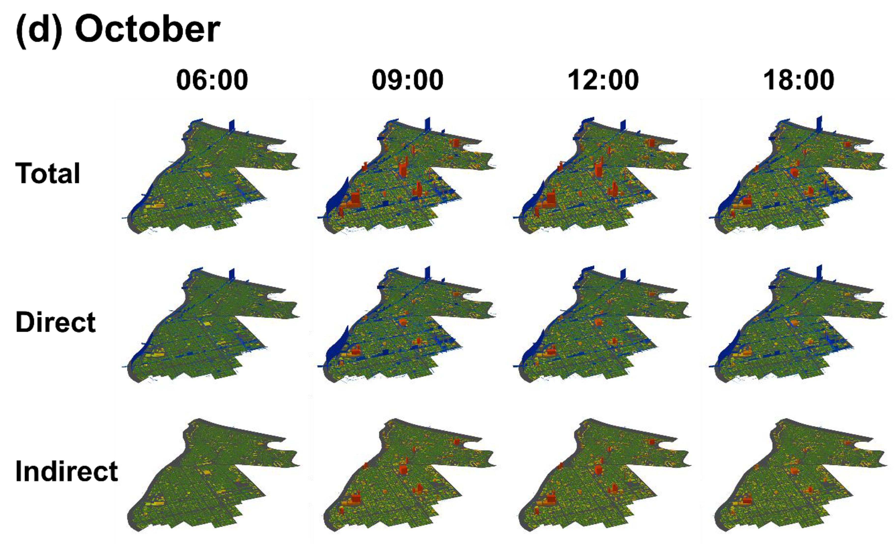
Figure 5 displays the estimated total, direct, and indirect carbon emissions at 06:00, 09:00, 12:00, and 18:00 in January, April, July, and October. Red represents emissions from individual buildings while blue represents emissions at each road link. The number of buildings and road links in our target area (Figure 1) were 46,352 and 7928, respectively. Supplementary material (CO2mapping.gif) displays annual average estimated total carbon emissions in 3D movie.
Our discussion of the results focuses on four viewpoints. Firstly, in terms of time, road emissions increased rapidly between 06:00 and 09:00, following which building emissions drastically increased and accounted for the majority of emissions until 18:00. This trend was caused by intensive commuting in the morning (06:00–09:00) and activities during working hours (09:00–18:00). Although road emissions also increased during evening commuting hours (15:00–18:00), these were lower than those in the morning. Secondly, regarding the seasons, building emissions in the summer (July) were remarkably larger than those in the other months, probably due to the high demand for cooling. This result suggests that low carbon management for cooling is the top priority. Furthermore, cooling management will be increasingly important as global warming advances. A comparison of cooling systems, such as greening and mist, will be an important first step to cost-effective cooling management. Building emissions in the winter (January) were slightly larger than those in autumn (October); suggesting effective heat management, e.g., using wasting heat is secondarily important based on the seasonal patterns of building emissions. Thirdly, in terms of direct or indirect emissions, building and road emissions showed totally different patterns. Regarding road emissions, direct emissions were dominant; this implies the potential of greatly decreasing transportation emissions if gasoline vehicles are replaced with electric vehicles (EVs), which do not emit direct emissions. This suggests the huge impact EVs can have. However, EVs increase indirect emissions through their electricity generation. Comparison of carbon maps before and after the installation of EVs will be an interesting future research topic, to visualize the impact of EVs. Finally, regarding places, building emissions were especially large in the Kinshi-cho area (see Figure 1), which is a principal commercial district. By contrast, somewhat unexpectedly, emissions from the SkyTree area, which is another commercial district, were estimated to be not very large; only one or two buildings indicated large emissions around SkyTree. Visualization using 3D carbon mapping is useful to help people intuitively correct their common sense-based misunderstandings, such as emissions in the SkyTree area being larger than the Kinshi-cho area. SkyTree’s smaller emissions are due to new energy-efficient buildings arranged in a well-planned zoning scheme. In contrast, Kinshi-cho’s large emissions are attributable to the unplanned, densely packed nature of the restaurant district. Regarding road emissions, a single bridge crossing the Ara river, a principal river, was estimated as significantly contributing to total emissions. The large emissions might be due to traffic congestion caused by vehicles attempting to cross the river. An interesting finding was that the bridge’s large emissions lasted throughout the day. The detection of such a hot spot is also an unexpected outcome that would never been found without carbon mapping.
These results show that visualizing temporal (seasonally and hourly) changes in a 3D manner would be useful to better understand current carbon emissions, thus facilitating the implementation of context-specific carbon emission management strategies for the purpose of reducing carbon emissions. Generally, citizens are often unaware of the carbon emissions from their activities because the emissions effects are not immediately visible. Therefore, this approach using spatial big data would be an effective tool to facilitate carbon management by local stakeholders such as municipality governments and companies, and to urge them to de-carbonize their activities.
4. Concluding Remarks
We showed that micro geodata are useful in estimating carbon emissions from individual buildings and roads that change over time, by visualizing them in a 3D manner. A benefit of micro geodata is its application in considering individual spatio-temporal activities on road networks and in buildings. Furthermore, when coupled with visualizing the data in a 3D manner it becomes easier to interpret the absolute and relative differences by height and colour. In value classification systems only using colours, we do not know the difference in magnitudes within the same class. Visualizing in a 3D manner could provide stakeholders, who want to implement certain strategies and reduce carbon emission, an easy-to-understand explanatory material for citizens as 3D figures are more easily interpretable and closer to human scale. However, our bottom-up approach did not consider carbon monitoring data, which are provided by the Carbon Dioxide Information Analysis Center [31], Greenhouse Gases Observing Satellite (GOSAT) project [32], and so on. In addition, on an urban scale, carbon dioxide sensors have often been distributed to monitor district-level carbon concentrations [33]. Integration of the bottom-up estimation with global and local monitoring, e.g., through data assimilation, would be an interesting research endeavour in the future.
Supplementary Materials
The following are available online at https://www.mdpi.com/2071-1050/10/12/4472/s1, CO2mapping.gif displays annual average estimated total carbon emissions in 3D movie.
Author Contributions
Conceptualization, Y.Y.; Data curation, Y.A.; Methodology, Y.Y., T.Y., D.M., and T.M.; Visualization, T.Y.; Writing—original draft, Y.Y., T.Y., and D.M.; Writing—review and editing, T.M. and Y.A.
Acknowledgments
This study was supported by joint research projects with Center for Spatial Information Science, the University of Tokyo (Research Numbers: 698 and 827). We appreciate Michael Tobey for his useful comments.
Conflicts of Interest
The authors declare no conflict of interest.
References
- Gurney, K.R.; Romero-Lankao, P.; Seto, K.C.; Hutyra, L.R.; Duren, R.; Kennedy, C.; Grimm, N.B.; Ehleringer, J.R.; Marcotullio, P.; Hughes, S.; et al. Climate change: Track urban emissions on a human scale. Nature 2015, 525, 179–181. [Google Scholar] [CrossRef] [PubMed] [Green Version]
- Gately, C.K.; Hutyra, L.R.; Wing, I.S.; Brondfield, M.N. A bottom up approach to on-road CO2 emissions estimates: Improved spatial accuracy and applications for regional planning. Environ. Sci. Technol. 2013, 47, 2423–2430. [Google Scholar] [CrossRef] [PubMed]
- Geertman, S.; Stillwell, J. Planning Support Systems in Practice; Springer: New York, NY, USA, 2003. [Google Scholar]
- Akiyama, Y. Applications of micro geodata for urban monitoring. In Proceedings of the 16th International Conference on Geographic Information Systems: Spatial Big Data Technologies and Applications for Future Society, Soul, Korea, 16 August 2014; pp. 103–116. [Google Scholar]
- Akiyama, Y.; Nishimoto, Y.; Shibasaki, R. Projecting future distributions of facility deserts for smart regional planning: A micro geodata approach in Japan. In Proceedings of the 15th International Conference on Computers in Urban Planning and Urban Management, Adelaide, Australia, 11–14 July 2017; p. 35081. [Google Scholar]
- Li, M.; Li, Z.; Vasilakos, A.V. A survey on topology control in wireless sensor networks: Taxonomy, comparative study, and open issues. Proc. IEEE 2013, 101, 2538–2557. [Google Scholar] [CrossRef]
- Rashid, B.; Rehmani, M.H. Applications of wireless sensor networks for urban areas: A survey. J. Netw. Comput. Appl. 2016, 60, 192–219. [Google Scholar] [CrossRef]
- Batty, M.; Axhausen, K.W.; Giannotti, F.; Pozdnoukhov, A.; Bazzani, A.; Wachowicz, M.; Portugali, Y. Smart cities of the future. Eur. Phys. J. Spec. Top. 2012, 214, 481–518. [Google Scholar] [CrossRef] [Green Version]
- Batty, M. Big data, smart cities and city planning. Dialogues Hum. Geogr. 2013, 3, 274–279. [Google Scholar] [CrossRef] [PubMed] [Green Version]
- Batty, M. Big data and the city. Built Environ. 2016, 42, 321–337. [Google Scholar] [CrossRef]
- Yamagata, Y.; Murakami, D.; Yoshida, T. Dynamic urban carbon mapping with spatial big data. Energy Procedia 2017, 142, 2461–2466. [Google Scholar] [CrossRef]
- Sharifi, A.; Yihan Wu, Y.; Khamchiangta, D.; Yoshida, T.; Yamagata, Y. Urban carbon mapping: Towards a standardized framework. Energy Procedia 2018, 152, 799–808. [Google Scholar] [CrossRef]
- Goodchild, M.F. Citizens as sensors: The world of volunteered geography. GeoJournal 2007, 69, 211–221. [Google Scholar] [CrossRef]
- Li, W.; Li, L.; Goodchild, M.F.; Anselin, L. A geospatial cyberinfrastructure for urban economic analysis and spatial decision-making. ISPRS Int. J. Geo-Inf. 2013, 2, 413–431. [Google Scholar] [CrossRef]
- Miller, H.J.; Shaw, S.L. Geographic information systems for transportation in the 21st century. Geogr. Compass 2015, 9, 180–189. [Google Scholar] [CrossRef]
- Kraak, M.J. Computer-Assisted Cartographical Three-Dimensional Imaging Techniques; Delft University Press: Delft, The Netherlands, 1988. [Google Scholar]
- Zhou, Y.; Dao, T.; Thill, J.C.; Delmelle, E. Enhanced 3D Visualization Techniques in Support of Indoor Location Planning. Comput. Environ. Urban Syst. 2015, 50, 15–29. [Google Scholar] [CrossRef]
- Shepherd, I.D.H. Travails in the third dimension: A critical evaluation of three-dimensional geographical visualization. In Geographic Visualization: Concepts, Tools and Applications; Dodge, M., McDerby, M., Turner, M., Eds.; John Wiley: Chichester, UK, 2008; pp. 199–222. [Google Scholar]
- Lovett, A.; Appleton, K.; Warren-Kretzschmar, B.; Haaren, C. Using 3D Visualization Methods in Landscape Planning: An Evaluation of Options and Practical Issues. Landsc. Urban Plan. 2015, 142, 85–94. [Google Scholar] [CrossRef]
- Lange, E. 99 volumes later: We can visualise. Now what? Landsc. Urban Plan. 2011, 100, 403–406. [Google Scholar] [CrossRef] [Green Version]
- Blaschke, T.; Donert, K.; Gossette, F. Virtual Globes: Serving Science and Society. Information 2012, 3, 372–390. [Google Scholar] [CrossRef] [Green Version]
- Bleisch, S.; Dykes, J.; Nebiker, S. Evaluating the Effectiveness of Representing Numeric Information Through Abstract Graphics in 3D Desktop Virtual Environments. Cartogr. J. 2008, 45, 216–226. [Google Scholar] [CrossRef] [Green Version]
- Kwan, M.P.; Lee, J. Geovisualization of human activity patterns using 3D GIS: A time-geographic approach. In Spatially Integrated Social Science; Goodchild, M.F., Janelle, D.G., Eds.; Oxford University Press: New York, NY, USA, 2004; pp. 48–66. [Google Scholar]
- Nakamichi, K.; Yamagata, Y.; Seya, H. An integrated model for assessing carbon dioxide emissions considering climate change mitigation and flood risk adaptation interaction. In Monitoring and Modeling of Global Changes: A Geomatics Perspective; Li, J., Yang, X., Eds.; Springer: Dordrecht, The Netherlands, 2015; pp. 241–262. [Google Scholar]
- The Greenhouse Gas Inventory Office of Japan. Available online: http://www-gio.nies.go.jp/ (accessed on 14 October 2018).
- Statistics Bureau, Ministry of Internal Affairs and Communications, Japan. Available online: http://www.stat.go.jp/english/index.html (accessed on 14 October 2018).
- Japan Institute of Energy. Cogeneration Plan and Design Manual; Japan Industrial Publishing: Tokyo, Japan, 2008.
- Zenrin, Co. Ltd. Available online: http://www.zenrin.co.jp/english/ (accessed on 14 October 2018).
- Agoop, Coop. Available online: https://www.agoop.co.jp/en/ (accessed on 14 October 2018).
- Environmental Systems Research Institute, Inc. Available online: https://www.esri.com/ (accessed on 14 October 2018).
- Carbon Dioxide Information Analysis Center. Available online: http://cdiac.ornl.gov/ (accessed on 14 October 2018).
- Yokota, T.; Yoshida, Y.; Eguchi, N.; Ota, Y.; Tanaka, T.; Watanabe, H.; Maksyutov, S. Global concentrations of CO2 and CH4 retrieved from GOSAT: First preliminary results. Sola 2009, 5, 160–163. [Google Scholar] [CrossRef]
- Mao, X.; Miao, X.; He, Y.; Li, X.Y.; Liu, Y. CitySee: Urban CO2 monitoring with sensors. In Proceedings of the IEEE INFOCOM, Orlando, FL, USA, 25–30 March 2012; pp. 1611–1619. [Google Scholar] [CrossRef]
Figure 1.
Study area: Sumida ward, Tokyo, Japan.

Figure 2.
Monthly energy consumptions (Source: Japan Institute of Energy [27]).
Figure 2.
Monthly energy consumptions (Source: Japan Institute of Energy [27]).

Figure 3.
Examples of Global Positioning System (GPS) points at 6:00, 9:00, 12:00, and 18:00 on 6 and 7 November 2016.
Figure 3.
Examples of Global Positioning System (GPS) points at 6:00, 9:00, 12:00, and 18:00 on 6 and 7 November 2016.

Figure 4.
GPS classification results on 7 November 2016 as an example: (A) OpenStreetMap; (B) the results around Tokyo SkyTree; (C) Walk; (D) Train; (E) Vehicle.
Figure 4.
GPS classification results on 7 November 2016 as an example: (A) OpenStreetMap; (B) the results around Tokyo SkyTree; (C) Walk; (D) Train; (E) Vehicle.

Figure 5.
Carbon mapping of total, direct, and indirect emissions at 06:00, 09:00, 12:00, and 18:00 in (a) January; (b) April; (c) July; and (d) October.
Figure 5.
Carbon mapping of total, direct, and indirect emissions at 06:00, 09:00, 12:00, and 18:00 in (a) January; (b) April; (c) July; and (d) October.


Table 1.
Estimated total carbon emissions in Sumida ward (kt).
| Emission Type | Residential | Non-residential | Transport |
|---|---|---|---|
| Direct | 113 | 167 | 421 |
| Indirect | 250 | 277 | 17 |
Table 2.
Annual energy consumptions (kWh/m2) (Source: Japan Institute of Energy [27]).
Table 2.
Annual energy consumptions (kWh/m2) (Source: Japan Institute of Energy [27]).
| Residence | Office | Retail | Hospital | Hotel | Sport facility |
|---|---|---|---|---|---|
| 21 | 156 | 226 | 170 | 200 | 210 |
© 2018 by the authors. Licensee MDPI, Basel, Switzerland. This article is an open access article distributed under the terms and conditions of the Creative Commons Attribution (CC BY) license (http://creativecommons.org/licenses/by/4.0/).
Share and Cite
MDPI and ACS Style
Yamagata, Y.; Yoshida, T.; Murakami, D.; Matsui, T.; Akiyama, Y. Seasonal Urban Carbon Emission Estimation Using Spatial Micro Big Data. Sustainability 2018, 10, 4472. https://doi.org/10.3390/su10124472
AMA Style
Yamagata Y, Yoshida T, Murakami D, Matsui T, Akiyama Y. Seasonal Urban Carbon Emission Estimation Using Spatial Micro Big Data. Sustainability. 2018; 10(12):4472. https://doi.org/10.3390/su10124472
Chicago/Turabian StyleYamagata, Yoshiki, Takahiro Yoshida, Daisuke Murakami, Tomoko Matsui, and Yuki Akiyama. 2018. "Seasonal Urban Carbon Emission Estimation Using Spatial Micro Big Data" Sustainability 10, no. 12: 4472. https://doi.org/10.3390/su10124472
Note that from the first issue of 2016, this journal uses article numbers instead of page numbers. See further details here.