Article

Responses of Urban Land Surface Temperature on Land Cover: A Comparative Study of Vienna and Madrid

1
Remote Sensing and Digital Earth Institute, Chinese Academy of Sciences, Beijing 100094, China
2
University of Chinese Academy of Sciences, Beijing 100049, China
3
Institute of Geography, Slovak Academy of Sciences, Bratislava 814 73, Slovakia
*
Author to whom correspondence should be addressed.
Sustainability 2018, 10(2), 260; https://doi.org/10.3390/su10020260
Submission received: 24 October 2017 / Revised: 10 January 2018 / Accepted: 11 January 2018 / Published: 23 January 2018

Abstract

:
The relationship between the land cover (LC) characteristics and the land surface temperature (LST) is significant for surface urban heat island (SUHI) study and for sustainability research. To better understand how the land surface temperature (LST) responds to LC, two urban areas, Vienna and Madrid, with different climatic conditions are selected and compared, using Landsat-8 OLI data and urban atlas data. To determine a suitable scale for analyzing the relationship between LC and LST, a correlation analysis at different sizes of spatial analytical scales is applied. To demonstrate the LC composition effects on LST, a regression analysis of the whole study area and in the specific circumstance is undertaken. The results show that: (1) In the summer, Vienna presents high temperature in the urban areas and low temperature in the surrounding rural areas, while Madrid displays the opposite appearance, being relatively cooler in the urban areas as compared to the rural areas, with the main different factors affecting elevated urban LST; (2) Suitable analytical scales are suggested in studying the LC–LST relationship between different LC characteristics in the two study areas; (3) Negative effects on the LST appear when the area of cooling sources, such as water or urban greenery, reaches 10% at a 990 × 990 m2 scale in Vienna. Built-up area is the main factor affecting elevated urban LST where such areas cover the majority at a 990 × 990 m2 scale in Madrid. These findings provide a valuable view regarding how to balance the urban surface thermal environment through urban planning.

Graphical Abstract

1. Introduction

Urban heat islands (UHIs) describe the phenomenon of atmospheric and surface temperatures being higher in urban areas than in surrounding rural areas [1,2]. T. J. Chandler began to study the factors that affected the urban climate in the 20th century by analyzing urban temperature data [3]. The problem of extreme UHIs was observed in cities worldwide, and was found to directly affect circulation inside the urban boundary layer [4,5] as well as human health [6]. Consequently, how to balance the urban thermal environment became a major research focusing on urban ecology and urban planning [7,8,9].
With the development of data acquisition technology, thermal remote sensing provides the radiative surface temperature information about the underlying surface and the interaction between the surface and the solar radiation [10,11]. The surface temperature significantly affects the urban thermal environment by modulating the temperature of the lowest layers of the urban atmosphere, and is therefore relevant in UHI study [12]. Land surface temperature (LST) retrieved by remote sensed data, which is a powerful indicator presently [13,14], becomes a convenient approach for studying the effects of the land cover to the surface temperature. However, the resolution of the commonly used thermal remote sensed data is not high, which reflects the knowledge limitation of the finer investigation of the urban environment or urban features.
The proposition that LST relates directly to the land surface characteristics [12,15,16,17] has been proven in numerous studies. Considerable research has been conducted concerning the effects of LC on LST and these studies have provided valuable insights into how land cover impacts the surface thermal environment, and what land cover composition can mitigate the extreme underlying thermal environment [13,17,18,19]. Researchers study the relevant effects using a variety of analytical units with different sizes such as grids or pixels, city blocks, sub-districts, or self-defined polygons. The compositions of the land cover in urban areas are complex, and the responses of the information retrieved by remote sensed data to various features are different. The differences of the scale between the retrieved information and other kinds of geo-information, as well as the different analytical scales existing in different studies, lead to the inconsistencies, which remain largely unaddressed in this kind of study [20,21,22,23]. Therefore, selecting an appropriate scale is significant, when we do the analysis of the information retrieved by remote sensed data and other kinds of geo-information.
New studies have evaluated the relationships between different LC values and LST at various scales, with a view to better understanding the scaling effects between LC and LST [18,24,25]. Quantifying the indeterminacy and complexity of the LST response to urban land cover requires a flexible and effective method of investigation, since suitable scales must also be selected to evaluate the composite effects [18,24,25,26]. Grid analysis is used in this study due to its flexibility of analysis with scale variation, bounding of quantitative values and locations, and statistics of area proportions in these regular shapes. Consequently, the relationships between LC and LST have been investigated using different spatial analysis scales [27,28,29,30]. As the spatial analysis scale increases in size, the land cover patterns in the grid unit change from simple to diverse patches with different combinations [25]. We aim to characterize the LC–LST relationship, based on the responses of LST at a different level of complexity in the land cover combination, in order to identify the most suitable scale at which to conduct the LC–LST analysis.
A number of studies have proved that the patterns of the urban thermal environment in different areas differ because of climatic divergences [26,31,32,33]. Previous studies have also demonstrated that the different appearances of the LST patterns are mostly caused by the differences in physical and biochemical properties of the land cover [32,33]. However, the inconsistency of these studies has, to the best of our knowledge, been less well-studied: the LST responses to one LC class can be different in various studies [15,32,34,35]. The reasons for the inconsistency can be concluded as due to two factors: (1) the standards of classification of land cover, and the resolution of the based LC image ranging from meter level to kilometer level; (2) the analytical conditions, for example, the difference between day and night [7,36] or different seasons [15], and different climatic conditions. Moreover, in studies relating to the responses of LST to LC, urban built-up areas and urban greenery are investigated by many researchers for their typical and significant heating and cooling impacts on surface urban heat islands (SUHIs) [6,18,20,23,37,38,39,40,41]. However, the anomalies of urban surface temperature are not caused by a single type land cover, but are the result of the combined impacts of multiple land cover patterns. In light of these inconsistencies, we select Vienna and Madrid as target cities, as they are distinct in terms of their climatic conditions, with detailed LC classes aggregated by the original land cover data with a harmonized legend and statistics frame. We aim to find not only the characteristic of the LST patterns, but also the factors affecting LST in the different climatic urban areas based on detailed land cover types.
Since UHI effects may cause energy waste [36,42] and an abnormal of local urban climate [4,5], thermal environmental considerations should play an important role in urban planning. The aim of this study is to solve the following questions: (1) How do LST patterns differ between cities with different climates? (2) What is the most influential factor affecting the surface thermal environment? (3) What analytical scale is suitable for analyzing the LC–LST relationship? (4) To what extent can land cover achieve the observed effects? To address these questions, we have attempted to determine the responses of LST to LC with a detailed LC classification, which concentrate on LST characteristics in different climatic conditions at various analytical scales, in order to identify a more appropriate land cover composition for urban design and planning.

2. Materials and Methods

In this study, we aim to obtain more comprehensive information about the relationship between LC and LST through three approaches:
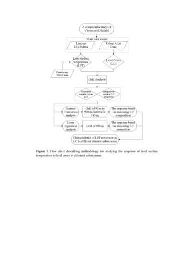
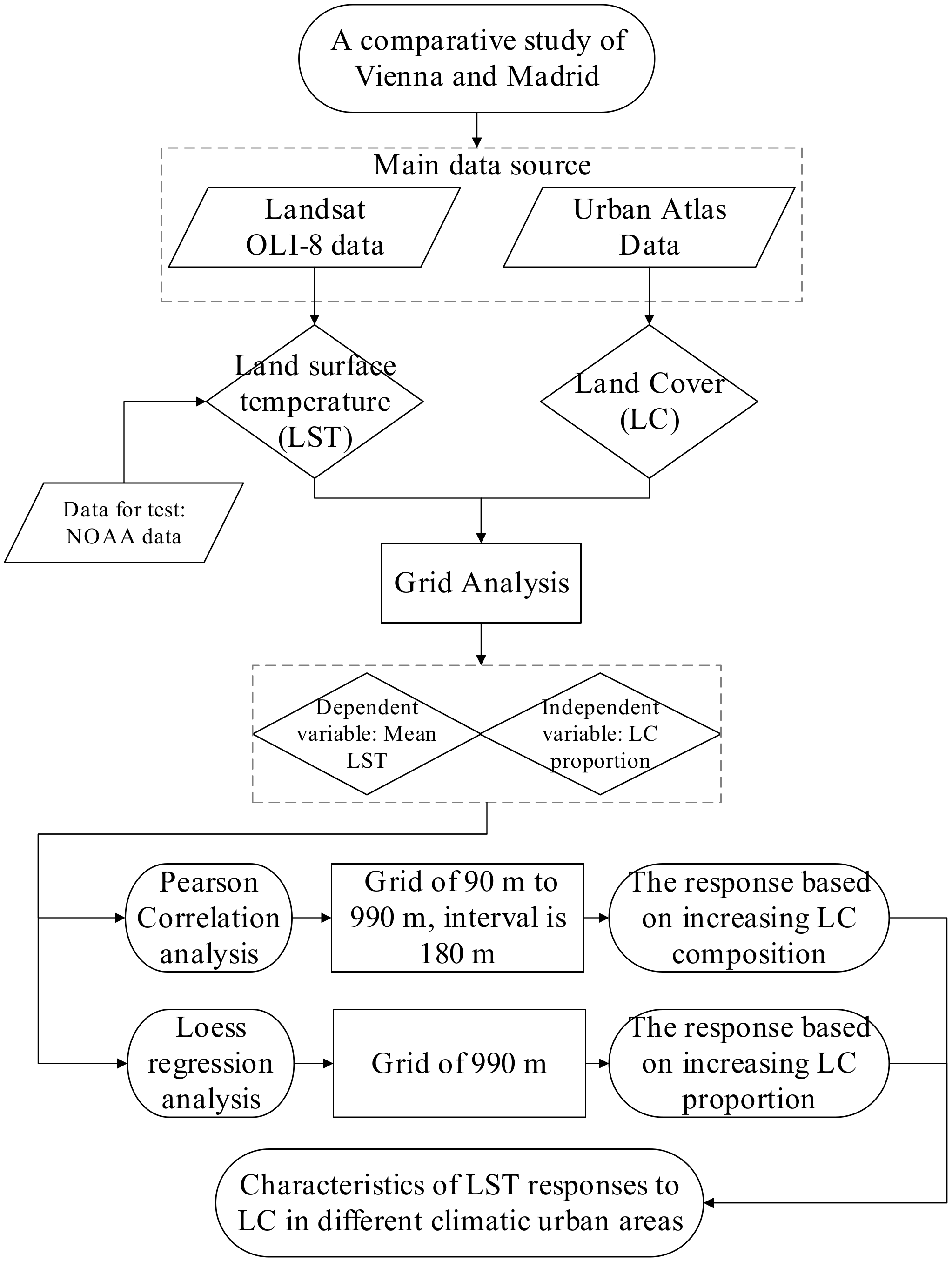
  • Comparing two study areas with different climates, to increase the credibility and comprehensiveness of the results, and to acquire a better understanding of the relationship between LCs and LST patterns in different climatic areas.
  • Accounting for the variability in vegetation, we use an NDVI-based emissivity method to calculate land surface emissivity, which is a critical value for LST [43,44].
  • Using grid analysis to build quantitative relationships between LST and LC at different analytical scales, to find a suitable scale for measuring the responses, by using the differences between the simple LC patterns at fine spatial analytical scales and the multiple LC combinations under larger spatial scales.
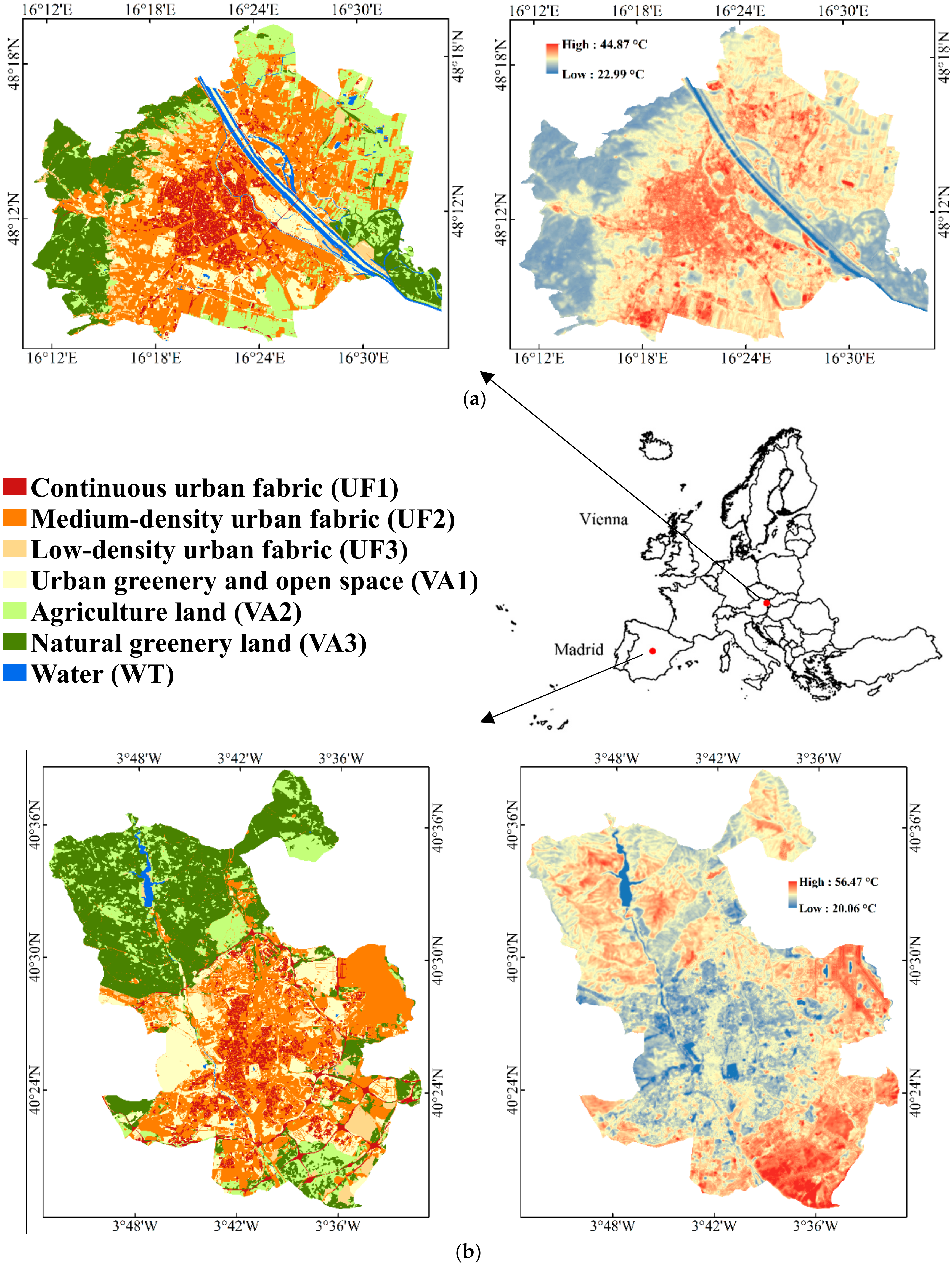
The flow chart about the materials and approaches of this study is showing in Figure 1.

2.1. Study Area

The study is conducted in two European cities with contrasting climatic conditions, Vienna and Madrid: Vienna has a humid continental climate [45], while Madrid has a hot-summer Mediterranean climate with continental influence [45]. The mean monthly value of the relative humidity in August is different between the two cities, as it is 68% in Vienna and 41% in Madrid [46]. Vienna, which has a large amount of urban open space and greenery [47], was named one of the world’s most livable cities by The Economist [48]. Madrid is the city with a high-level amount of urban trees and area of green surface per inhabitant [49]. The information about the study areas is showing in Table 1.
In a previous study, we investigated 15 European cities to find the cities with different climatic conditions, but with similar social conditions and land cover distribution. The general proportions of land cover types in the two cities are very close. The similar social conditions of the two cities, such as similar population density [50], and city size, make it possible to compare the relationship between LC and LST in different climatic conditions.

2.2. Data Sources and Image Pre-Processing

2.2.1. Land Cover Data and Aggregation

In this study, we map land cover based on the high-resolution land cover map data of the European Urban Atlas, which provides pan-European comparable land use and land cover data with the support of the European Space Agency and the European Environment Agency [51]. The harmonized legend and statistics frame of this product provide the opportunity to conduct analysis across different cities [52]. The data used in this study was collected and observed in 2012.
The Urban Atlas nomenclature contains 27 land cover classes. We focus on the urban fabric of different densities, the vegetation areas with different functions, and water land cover. Based on this consideration, we aggregate 27 categories into 7 types, including 3 types of urban fabric, 3 types of vegetation area and water land cover. The 7 types are: continuous urban fabric (UF1); medium-density urban fabric (UF2); low-density urban fabric (UF3); urban greenery and open space (VA1); agricultural land (VA2); natural greenery land (VA3); and water (WT). The rule used for aggregation is shown in Table 2.

2.2.2. Land Surface Temperature Retrieval

The LST data is derived from the thermal infrared (TIR) Band10 (10.30–11.30 µm, resolution of 100 m, resampled to 30 m) of Landsat-8 OLI [53]. A previous study showed that the effects of UHI effects are more drastic in summer [54]. Moreover, as summer has the largest canopy of vegetation, it offers an opportunity to analyze the effects of green space on LST [55]. Based on these considerations and the time correspondence to Urban Atlas data, we utilize data from the summer of 2013 (1 June to 31 September) to study the relationship between LC and LST. Three and five images taken under clear atmospheric conditions were acquired during this period in Vienna and Madrid, respectively. The data acquisition times are 9:05 a.m. Greenwich Mean Time (GMT) in Vienna and 10:45 a.m. GMT in Madrid. The information of the images is shown in Table 3.
Land surface emissivity (LSE) is a determining factor in the LST estimating process [15,18,56,57]. Recent studies have addressed the relationship between LST and surface characteristics via vegetation indices [30,58,59]. Valor and Caselles proved that LSE relates to Normalized Difference Vegetation Index (NDVI) and is capable of explaining the experimental behavior of LST [60]. To calculate LST, fundamental surface descriptors such as NDVI are used instead of qualitative LC classes, due to their better biophysical expression [43,44]. Therefore, an NDVI-based emissivity method (NBEM) is used in this study to calculate the LSE [61,62]. In order to obtain the LST, the following process of calculation are used:
  • Calculation of the Top of Atmospheric radiance (TOA);
  • Transformation of spectral radiance to blackbody temperature ( T B );
  • Calculation of NDVI;
  • Calculation of the fractional vegetation cover ( P V )
  • Calculation of LSE;
  • Calculation of LST.
We calculate the TOA, T B and NDVI values during the basic image processing. Based on the calculation, the fourth step is the calculation of the fractional vegetation cover—Pv value:
P V = [ NDVI     NDVI min NDVI max + NDVI min ] 2
where NDVImin = 0.2 and NDVImax = 0.5 are the NDVI values for bare soil and full vegetation, respectively.
An NDVI thresholds method with Pv is used for LSE estimation from Landsat OLI8 imagery as the following equation [43,60]:
ε = { a ρ r e d + b   ,                                         NDVI < 0.2       ε v P V + ε s ( 1 P V ) + C ,     0.2 NDVI 0.5 ε v + C ,                                                     NDVI > 0.5      
The value of a and b on band 10 of Landsat OLI8 derived from MODIS UCSB (University of California, Santa Barbara, CA, USA) emissivity library is a = 0.047 and b = 0.973 , when the pixel is considered as bare soil (PV = 0 which is the representation of NDVI < 0.2).   ε v and ε s are emissivities of vegetation and soil for band 10 of Landsat OLI8, which are also calculated from the MODIS UCSB emissivity library. ε v = 0.9863 ; ε s = 0.9668 .   C in Equation (2) is a term which takes the cavity effect into account due to the surface roughness (C = 0 for flat surfaces). Sobrino et al. suggest that C can be estimated as following [30,63]:
C = ( 1 ε s ) ε v · F · ( 1 P V )
where F is the geometrical factor which is typically 0.55.
Further, with the result of LSE, the land surface temperature is estimated by this equation as following [30,63]:
LST =   T B /   [ 1 + ( λ T B ρ ) ln ε ]
where:
  • T B = Black body Temperature;
  • λ = Wavelength of emitted radiance;
  • ρ = h × c/σ =1.438 × 10⁻² mK (σ = Boltzmann constant = 1.38 × 10⁻²³ J/K, h = Planck’s constant = 6.626 × 10⁻³⁴ Js, c = velocity of light = 2.998 × 10⁸ m/s);
  • ε = Land surface emissivity (LSE)
We calculate the LST result of each image in order to obtain the average LST result, which represents the summer LST of the study areas.
In addition, NOAA hourly climate data [64] is used to exclude the uncertainty of weather factors. There are three weather stations in Vienna and two in Madrid. Checking the NOAA data demonstrated that there was no extreme weather locally in the 72 h before the acquisition of the image. Therefore, the LST result can be considered to be credible.

2.3. Statistics

Since the LST response is a consequence of multiple LCs, the relationship between LST and LC can be highlighted and quantified by changing the size of spatial analytical scale. The principal aim is to investigate a suitable scale for LC–LST relationship analysis, and to determine the impacts of LC composition on LST via the change of LST responses with simple to complicated LC combinations. It can be analyzed according to the following steps:
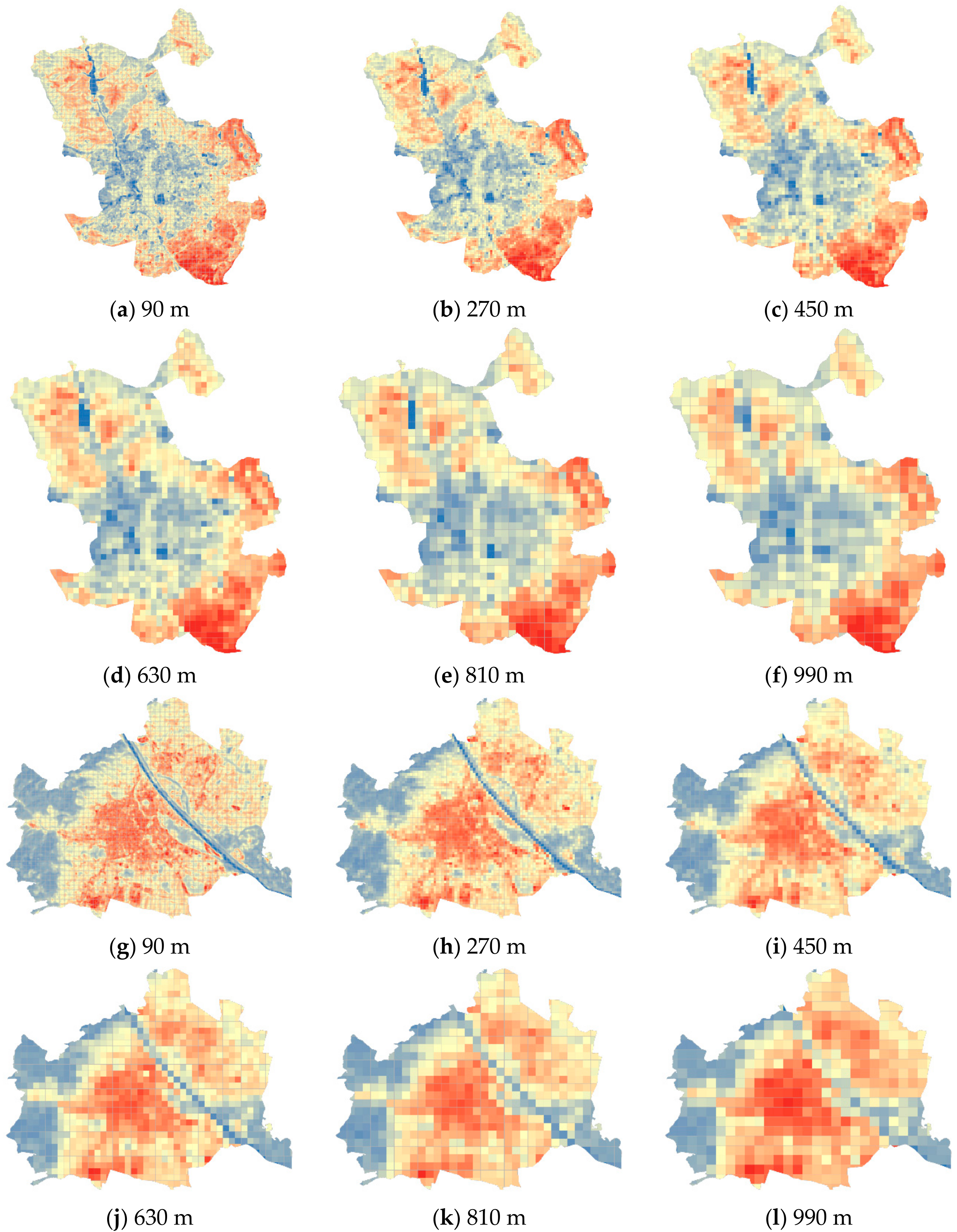
  • The original LST images are resampled at six spatial scales with the following grid sizes: 1. 90 × 90 m2 (3 × 3 pixels); 2. 270 × 270 m2 (9 × 9 pixels); 3. 450 × 450 m2 (15 × 15 pixels); 4. 630 × 630 m2 (21 × 21 pixels); 5. 810 × 810 m2 (27 × 27 pixels); 6. 990 × 990 m2 (33 × 33 pixels). We build the grids with six different sizes based on the template extent of the study area with the origin coordinate. Then, the mean LST of each grid at the six scales is extracted with the spatial statistics tool (zonal statistics) of ArcGIS 10.2, and the resulting images are shown in Figure 2.
  • We acquire the mean LST of each grid as the dependent variable, and the proportion of each LC type on the corresponding grid as the independent variable. A Pearson correlation analysis is firstly conducted at each of the analytical scales to identify the correlation coefficient between the LST and the proportion of each LC. With the increase of the spatial scale, the resulting analysis allowed for the determination of the change of the LST-LC correlation coefficient based on variable LC combinations, which provides an interpretation of the suitable scale for analyzing the LC–LST relationship.
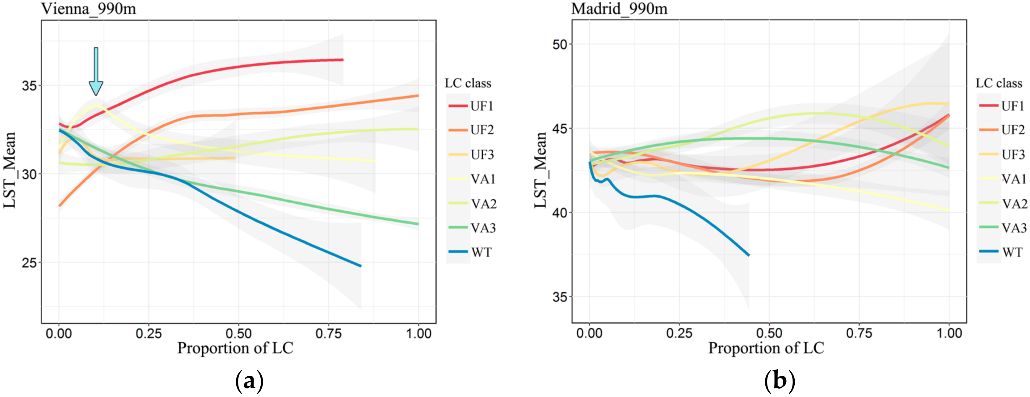
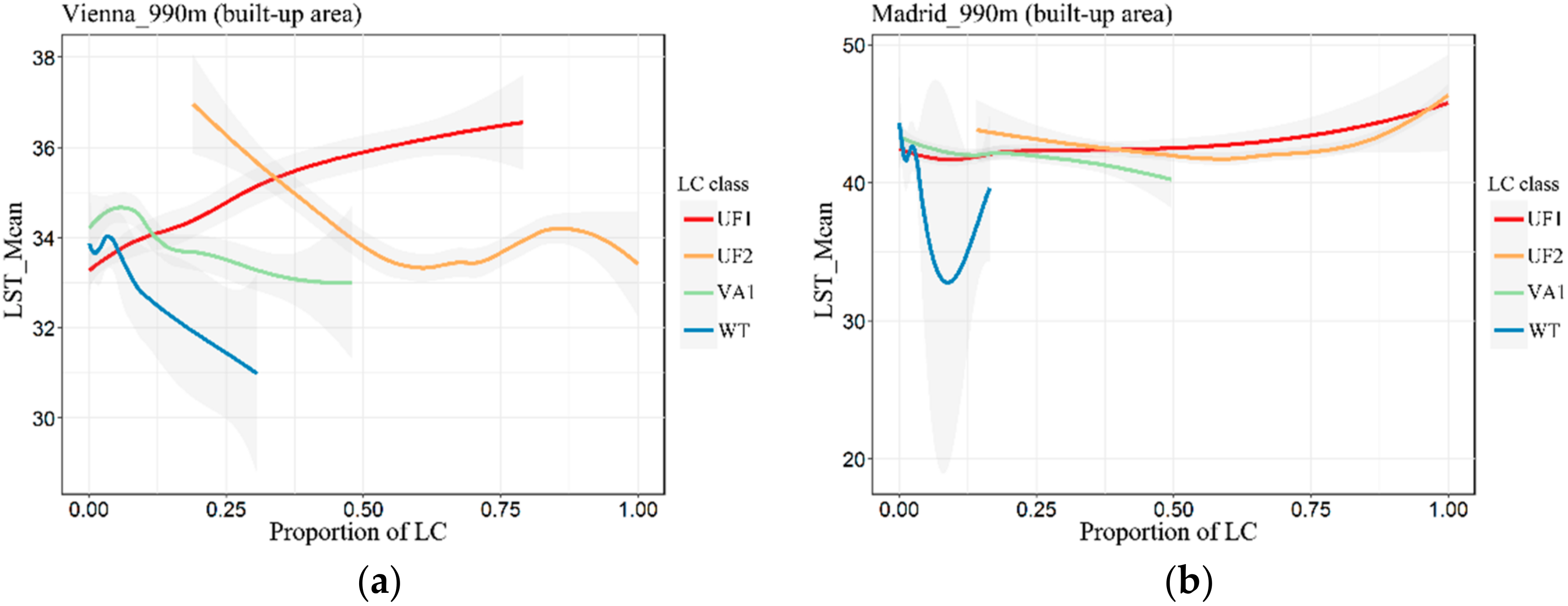
  • A Loess regression analysis is next applied to reveal the characteristics of LST responses based on a changing LC proportion, with attention paid to the LC compositions that display negative or positive effects on LST. We select the spatial analytical scale of 990 × 990 m2 due to its advantage of combination expression to analyze the combined effects.
At the 90 m scale, which size is much smaller than the land cover patches, the analysis at this scale signifies the response of LST at relatively simple LC combinations. As the size of the spatial analysis scale increases, more types of LC are contained in the grid, and the combinations are more complicated. At the analytical scale of 990 m, we find that 95.4% of the grids in Vienna and 94.1% in Madrid are covered by multiple LC classes.

3. Results

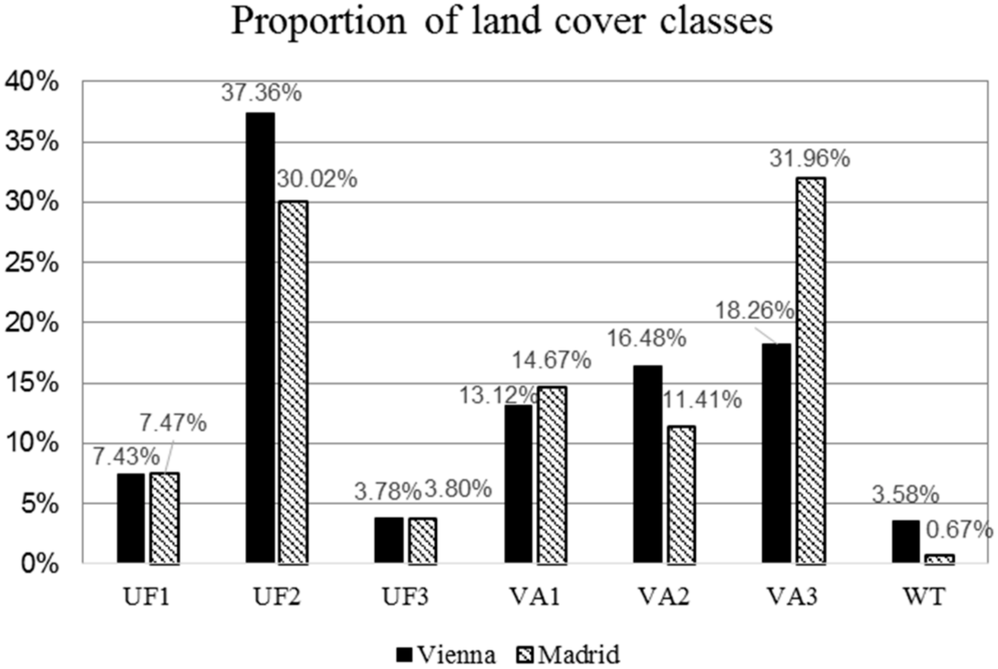
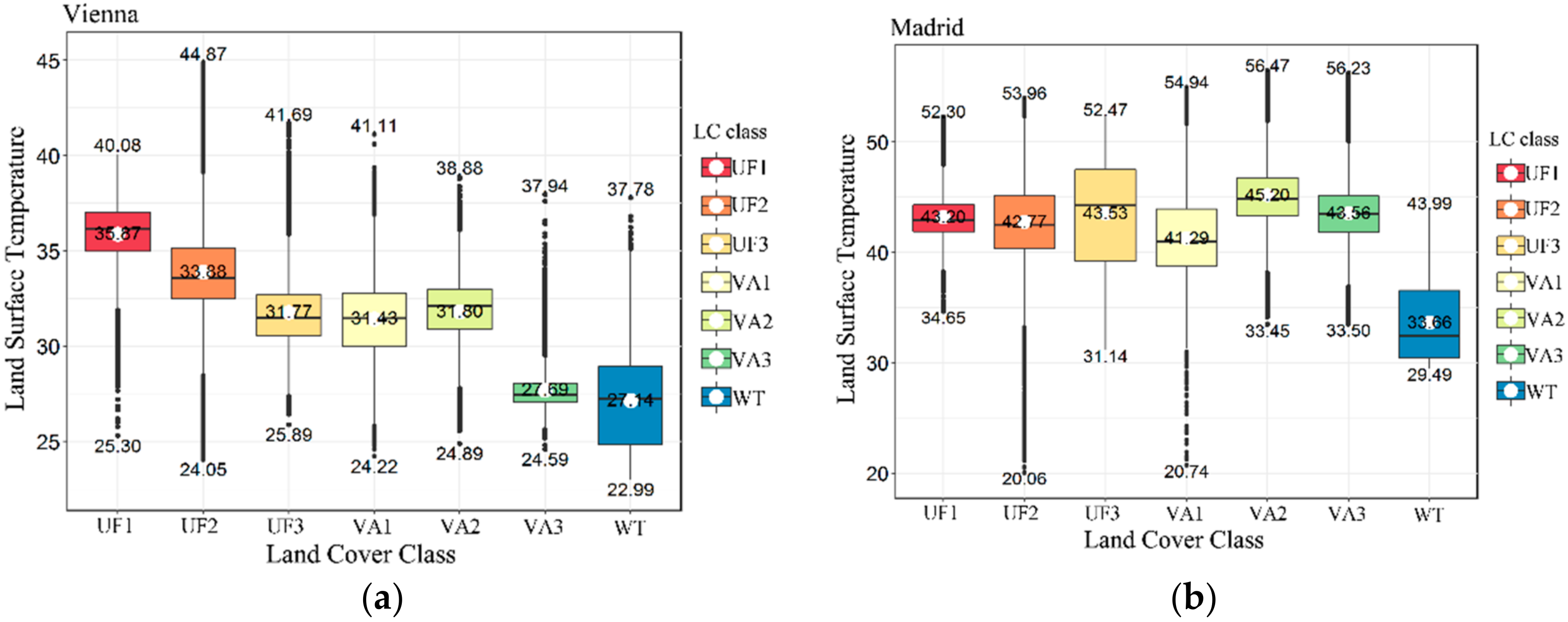
3.1. The Distribution and Characteristics of LC and LST in the Two Study Areas

After the aggregation from 27 to 7 LC classes based on the rule in Table 2, and the calculation of the summer LST of the two study areas, we map the result on the land cover maps and LST images. The results are shown in Figure 3. The proportion of each LC classes in the two study areas is calculated and shown in Figure 4.
Figure 4 shows that the proportion of the seven LC classes in the two study areas are similar, which is one of the reasons for choosing these two cities for comparative analysis. The main difference between the two cities is that the proportion of natural greenery land (VA3) is higher in Madrid than Vienna, by 13.70%. Moreover, the species of VA3 are different in the two cities: a large area of grassland and shrubbery is distributed in the north of Madrid [65], while the main type of VA3 in Vienna is forest [66].
From Figure 3, we can observe that the city center shows a higher temperature in Vienna. The response of continuous urban fabric (UF1) is significant, and the LST decreases from the center to the rural areas covered with natural greenery land (VA3) and agricultural land (VA2). The figure shows that the cool temperature patches correspond to water (WT) and urban greenery and open space (VA1) inside the city. In Madrid, the opposite phenomenon of LST pattern appears. There is a higher temperature in the rural areas, and a relatively lower temperature in the urban areas. There is no obviously high LST patch inside the city. The high-temperature patches appear in the north, northeast, and south, outside of the urban built-up area, corresponding to natural greenery land (VA3), and the areas of mixed with VA3 and agricultural land (VA2).
To obtain detailed information about the different LST response to each LC, the minimum, maximum, and mean values of LST based on each LC types are calculated and shown in Figure 5. The range of LST value calculated in the whole study area is 14.53 °C higher in Madrid than in Vienna. The highest temperature was observed in medium-density urban fabric (UF2) in Vienna and in agricultural land (VA2) in Madrid.
In terms of the urban fabric areas, the mean LST value order is greatest in UF1, then UF2, and lowest in UF3 (continuous to low-density urban fabric). In Madrid, low-density urban fabric (UF3) has the highest mean LST value, followed by continuous urban fabric (UF1), with the lowest in medium-density urban fabric (UF2). In Vienna, the mean LST values are similar for UF3, urban greenery and open space (VA1), and agricultural land (VA2). The mean LST of natural greenery land (VA3) is 3.73 °C lower than urban greenery and open space (VA1) in Vienna, but 2.26 °C higher in Madrid. In addition, the mean LST of VA1 is the lowest among all LC types except water (WT) in Madrid. The mean LST of natural greenery land (VA3) is slightly higher than that of water in Vienna, while the value of WT is significantly different from the other LCs in Madrid. Water (WT) has the lowest mean LST in the two study areas, while the highest mean LST values were observed in UF1 in Vienna and VA2 in Madrid.

3.2. The Relationship of LC to LST in Different Spatial Analysis Scales

A Pearson correlation analysis is carried out with LC proportion, mean LST values at increasing spatial scale. The correlation coefficients can demonstrate the responses of LST on increasing complexity of LC combinations, through providing information at different spatial scales. The correlation coefficients of LST and LC are presented in Table 4 and Table 5.
The results are illustrated and discussed in three parts: urban fabric area (UF1/UF2/UF3); vegetation area (VA1/VA2/VA3); and water (WT).
(1)
Urban fabric area (UF1/UF2/UF3) contrast: For Vienna, the correlation coefficient between LST and LC is highest in continuous urban fabric (UF1), at all analytical scales. The positive correlation coefficients of UF1 and medium-density urban fabric (UF2) increase as the spatial scale increases in size. The low-density urban fabric (UF3) in Vienna does not clearly correlate with LST, and it shows a negative correlation coefficient when the scale of analysis is over 270 m. In Madrid, there is no significant correlation for any of the three kinds of urban fabric, including UF1 and UF2, in contrast to Vienna. Moreover, the correlation coefficients do not differ significantly as the scale of analysis increases.
(2)
Vegetation area (VA1/VA2/VA3) contrast: Urban greenery and open space (VA1) and natural greenery land (VA3) show negative correlations, and agricultural land (VA2) shows a positive correlation with LST, under all analytical scales in the two study areas. For Vienna, the correlations between LST and VA3 are stronger than VA1 and VA2 across all the analytical scales. In addition, the correlation coefficients of VA1 and VA3 are very similar at the 90 m scale of analysis, in which the interior LC type is relatively simple. As the analytical scale increases, the correlation coefficients of VA1 and LST decline, while the correlation coefficients of VA3 increase. For Madrid, the correlation coefficients of the three kinds of vegetation area are all relatively low. It can’t be ignored that VA1 has the second most negative correlation coefficient (lower than water). With the increase of the scale, the negative correlation coefficients of VA1 to LST increase, in diametric opposition to Vienna.
(3)
Water (WT) contrast: The correlation coefficients of WT are notable in the two cities at all analytical scales, which indicates significant cooling effects. In Madrid, the correlation coefficients between LC and LST are all below 0.3, except for WT, for which the correlation coefficient is significantly different. The correlation coefficient is highest at the analytical scale of 270 m. The correlation coefficient of WT is lowest at the analysis scale of 990 m.
The correlation coefficients between LST and each LC are higher in Vienna than in Madrid, and the variation across the seven LC classes and six analytical scales are more obvious.

3.3. The Effects of LC in Specific Urban Combinations

Based on the results, we choose the largest analytical scale (990 m × 990 m) to evaluate the effects of LC composition on LST, because of the advantage it offers in terms of combination expression. Simple Loess regression lines are generated in the LC proportion, mean LST-regression diagram. The results are as follows:
Figure 6a illustrates that in Vienna, the mean LST of the grid responds negatively at all LC proportions to an increase in natural greenery land (VA3) and water (WT) proportion, which indicates that VA3 and WT have a cooling effect independent of area size. Mean LST increases as the proportions of UF1 and UF2 increase. However, we found that mean LST and urban greenery and open space (VA1) are at first positively correlated at low proportions, and then negatively correlated at higher proportions, with a peak at around 0.1.
Figure 6b illustrates that both continuous urban fabric (UF1) and medium-density urban fabric (UF2) are negatively correlated at low proportions and positively correlated at higher proportions with LST. The LC which has the main cooling effects on the urban built-up area in Madrid is water (WT), as shown in Figure 6b. However, the proportion of WT in the total urban land cover is low, and there is no grid that is mostly covered with water. Notably, that the LST response to urban greenery and open space (VA1) is negative at all LC proportions. The relationships between LST and agricultural land (VA2) and natural greenery land (VA3) are first positive and then negative, with a gradual inflexion. The inflexion of VA3 occurs before that of VA2.

4. Discussion

4.1. Characteristics of LST Patterns and the Factors Affecting LST in Different Climatic Areas

The urban thermal environments of different areas differ because of climatic divergences, a point which has been proved by many researchers such as Yang, Q, Zhou, D and others. [26,31,32,33]. The SUHI phenomenon can be found in the majority of cities, while the surface urban cool island (SUCI) phenomenon is observed in some areas such as Mexico City [32]. Differences of LST patterns in the two climatic areas are also presented in this study. The research regarding the Madrid SUHIs carried by José A. Sobrinoa demonstrated that low SUHI values (sometimes negative values) are obtained at noon, since the rural surfaces appear warmer than the urban ones [16]. We can clearly see that Vienna presents higher temperatures in the center of the city with lower temperatures around the city. However, in Madrid, the typical urban hot spots do not appear and instead the opposite trend occurs such that it is cooler in the center of the city compared to the rural areas.
The main factors affecting elevated urban LST of the two cities are different. Generally, the anthropogenic landscape is considered to be one of the main causes of high LST, and vegetation area and water area are considered to be the cooling sources for the thermal environment [13,67,68,69]. The continuous urban fabric (UF1) and medium-density urban fabric (UF2) are indeed strongly correlated with LST in Vienna, but in Madrid, built-up areas are not the primary determinant of the urban-rural thermal environment, but instead agriculture land cover (VA2), which is a type of vegetation area, is the factor affecting elevated LST. Water shows a significant negative correlation with LST in the two cities, especially in Madrid, and water land cover is the most significant cooling source.
The research regarding the urban local climate of Vienna carried by Milena Vuckovic, put forward the further suggestion that the UHI phenomenon can vary considerably depending on such factors as urban density, surface properties, extent of vegetation, etc. [7,70]. Figure 5 reveals that, in Vienna, the urban fabric area with higher urban fabric density shows a higher LST with obvious differences. Combined with Table 4, the correlation coefficients are continuous urban fabric (UF1) > medium-density urban fabric (UF2) > low-density urban fabric (UF3) across all scales of spatial analysis in Vienna, which is the same order as the mean LST value (Figure 5). While in Madrid, the low-density urban fabric (UF3) shows a higher temperature compared to the continuous urban fabric (UF1) and medium-density urban fabric (UF2) which are in the city center.
The hypothesis that urban vegetation types affect the thermal environment [58] has been supported by several studies. An experiment carried out by Krehbiel proved that the annual cropland has seasonal impacts on UHIs [71]. In this study, we observe that although urban greenery and open space (VA1), agricultural land (VA2), and natural greenery land (VA3) are all types of vegetation area, these three LC classes impact LST differently. For instance, the agricultural land (VA2) has relatively high positive effects on LST in the two study areas, especially in Madrid, where many farmlands are harvested in summer. Additionally, the relationship between LST and the vegetation areas inside and outside of the city are different. The LST of vegetation areas outside the city, which are mostly classified into natural greenery land (VA3), is much lower than that of urban greenery and open space (VA1) areas, which are located inside the city in Vienna. However, this relationship is the opposite in Madrid. Rural areas in both Vienna and Madrid are covered by natural greenery land (VA3), but with different vegetation species, which could explain the different LST responses to VA3 in the two cities.

4.2. Characteristics of LST Responses to Land Cover: Difference between Cities and Various Analytical Scales

The different analytical scales that have been employed in various studies lead to an inconsistency in the analysis of the LC–LST relationship. To better understand the relationship, a number of studies have evaluated the relationship of different LCs with LST at various scales [18,24,25]. Here, we undertake the research employing analysis at different spatial scales to investigate the impacts of scale with two aims: to quantify the relationships between LST and LCs at various analysis scales, and to find a suitable scale for measuring these relationships.
The correlation coefficients of continuous urban fabric (UF1) are significant and increase with the increasing scale. The correlation coefficients of medium-density urban fabric (UF2) increase to the highest value when the scale increase to 810 m. Low-density urban fabric (UF3) has a low correlation coefficient with LST at all scales. Through the results, the relationship between urban fabric area and LST can be highlighted at a large scale. The results also demonstrate that an urban fabric with a higher building density shows more persistent positive effects on LST. In Madrid, the three kinds of urban fabric areas show low correlation coefficients with LST, especially the continuous urban fabric (UF1). The difference between the three kinds of urban fabric areas is not notable.
Moreover, the correlation coefficients of urban greenery and open space (VA1) and natural greenery land (VA3) in Vienna are very similar at fine scales. As the scale increases, the correlation coefficients of VA1 decrease, while the correlation coefficients of VA3 increase. This may be due to the urban greenery and open space (VA1) areas are at a smaller mess, which are mostly located in the urban zone. With the surrounding environment, which is covered by built-up areas or other urban facilities, VA1 shows a weakening negative correlation compared with the VA3 outside the city. In Vienna, the natural greenery land (VA3), which has the larger canopy and biomass of forest, displays the most significant negative impact on LST, even showing higher correlation coefficients than water at large spatial scales with a complex combination. According to this result, we suggest using a large scale to analyze the relationship between natural greenery (VA3) and LST, but a small scale for urban greenery and open space (VA1). In Madrid, the correlation coefficients of all the vegetation areas are not significant. The negative impacts on LST of the vegetation areas in the urban zone, which are mostly classified as VA1, are relatively larger than the other LC types.
In Vienna, the correlation coefficients of water (WT) and LST are all above 0.6 at all scales except the scale of 90 m. While, in Madrid, the correlation coefficients of water (WT) and LST are all significant but decline as the scale increases, up to a scale of 270 m. This may due to the average size of the water landscape is small in Madrid, which calculated as 115,664.02 m2. This area accounts for 57% of the single grid at the scale of 450 × 450 m2. When the area of the analytical scale is much larger than the patch area, the impacts of LC are reduced. Water resources in arid areas are particularly rare, which indicates that there is no sizable water parcel in the urban area to perform the cooling function. It is more suitable to use a fine scale to analyze the effects of water in Madrid.
Overall, the correlation coefficients of LC and LST in Vienna are relatively more significant than the correlation coefficients in Madrid. And the differences between the correlation coefficients for different LC classes are relatively larger in Vienna. Continuous urban fabric (UF1) and natural greenery land (VA3) have the most significant positive and negative correlation coefficient with LST. The correlation coefficients of the two LCs increase to the peaks at a scale of 990 m. Therefore, for Vienna, a scale between 810 m and 990 m is suggested to quantify the relationship of LC and LST. In Madrid, the negative correlation between water (WT) and LST is obvious, and the correlation coefficients of other LCs, either positive or negative, are not significant. Considering this, for Madrid, an analytical scale of the size between 270 m and 450 m is suggested for use in the study of LC–LST relationship.

4.3. The Effects of Land Cover Composition on LST in Two Urban Areas and Further Suggestion for Urban Planning

Previous studies have shown that LST is directly influenced by land surface characteristics [12,15,16,17,72], which includes the attribute, shape, composition, and configuration of land cover (LC) [34,69,73]. We observed that Madrid shows a low LST in built-up areas. To what extent can built-up areas display positive effects on LST at local scale? The effects of urban greenery and open space (VA1) decline with increasing scale in Vienna. What composition of urban greenery is necessary to perform a cooling function and to regulate the temperature? We found answers to these questions in a detailed study based on a regression analysis of LC proportion and mean LST at the 990 m analytical scale.
Although Madrid shows a relatively low temperature in built-up areas, the high cover of built-up areas is a potential factor of affecting elevated LST. Figure 6 demonstrates that the relationships between LST and the cover of urban fabric areas (UF1 and UF2) are first negative and then positive with an increasing of proportion, which indicates that the built-up areas will still be a factor in the formation of high LST when the urban fabric areas (UF1 and UF2) cover the majority of the analytical grid.
The urban greenery area has strong negative effects on LST which can counteract the impacts of the built-up areas. Some studies, for instance, Skoulika, F. researched on the relationship of thermal characteristics and urban park size, and have shown that the parks must reach a certain size in order to contribute a more obviously to a thermostat effect [74]. In Figure 6, we can observe that the cooling effects of urban green and open space (VA1) appear when the total area accounts for more than 10% of the grid in Vienna.
Here, we aim at giving detailed composition suggestions regarding urban greenery and water areas, which can be considered as cooling sources, to balance the thermal environment. To study the effects of different LC combinations, and to verify the results in specific urban environments, we select a grid of built-up areas based on urban fabric proportions. We then display four LC classes (UF1, UF2, VA1, and WT), which are located in the urban area. The selection condition and results are showing as follows:
Urban built-up area: The summed proportion of UF1 and UF2 is above 50%.
In Figure 7, the urban greenery and open space (VA1) and water (WT) areas in the grids (which are selected to be a majority of urban fabric) of Vienna have inflexions. The results verify the conclusion that the cooling sources, such as water and urban greenery, have a negative influence on LST when their proportions reach a certain level. In Madrid, the temperature of built-up areas is over 45 °C, when the proportion reaches to a high level, which indicates a highly thermal risk in built-up areas. The water-LST relationship in built-up areas is unstable. Moreover, the urban greenery and open space (VA1) displays a negative effect on LST at all proportions of built-up areas.
Based on the above analysis, we put forward several suggestions for urban planning. For Vienna, the building density ratio should be a focus. The contiguous high-density building is likely to cause highly thermal patches. Incorporating urban greenery, open spaces, and water should be prioritized in urban planning in Vienna, since these land cover types play a significant role in mitigating temperature in high-density urban fabric areas. To effectively mediate urban surface temperature, more than 10% of the area at the 990 × 990 m2 scale should consist of the patches of these cooling sources. For urban planning in Madrid, the thermal effects of the farmland during the period after harvest and the low-density residential areas located on the urban fringe should be considered. Although the built-up area is cooler than the rural area, the heating effects inside the city should not be ignored. The urban fabric of high density becomes the main factor when its proportion is over 50%. Studies have shown that urban planners are trying to build parks in arid areas to maintain the SUCI and regulate the urban local climate [74]. Since the water scarcity in the arid areas in Madrid, the ability of urban greenery to play a regulating function should be fully acknowledged in urban planning.
There are still shortcomings and deficiencies of this study. Using more urban areas as case studies would be more sufficient. A follow-up study will investigate the current study areas in other seasons. Moreover, the study is being expanded to cover Munich, London, Paris, Amsterdam, and other cities, in order to elicit more detailed information about the relationship between land cover and land surface temperature.

5. Conclusions

Vienna and Madrid have been selected as case studies to address the suitable scale for the analysis of the relationship between LC and LST, due to their different climatic conditions. They are analyzed with remote sensing and land cover data as follows: (a) LST patterns are analyzed by comparing LST maps and land cover maps; (b) the correlation coefficient of LC proportion and mean LST is obtained at the increasing scale (increase from 90 m to 990 m in 180 m interval) to determine a suitable analytical scale for the study of LC–LST relationship; (c) detailed analysis is conducted at the 990 m scale and a specific grid with over 50% built-up area to demonstrate the composite effects. This last step enables us to analyze the effects of land cover composition on LST with a regression analysis of LC proportion and mean LST. The main results of the study are as follows:
(1)
In summer, Vienna presents high temperatures in the urban areas and low temperatures in the surrounding rural areas. The continuous urban fabric area (VA1) shows the strongest positive correlations with LST. Madrid displays relatively cooler in urban areas compared to rural areas. Water (WT) is the most negative factor affecting LST. None of the correlation coefficients between other LC classes and LST is above 0.3 in Madrid.
(2)
Suitable analytical scales are suggested for studying the LC–LST relationship between different LCs and different study areas. In Vienna, to analyze the urban fabric areas (UF1 and UF2) and natural greenery land (VA3) a large scale is appropriate, but a fine scale should be used for urban greenery and open space (VA1). In Madrid, we suggest using a relatively fine analytical scale to study the effects of water (WT), since the correlation coefficients of water (WT) decreased when the analysis scale exceeded 270 m. Considering the main factors affecting LST in the two study areas, for Vienna, the analytical scale between 810 m and 990 m is suggested to quantify the relationship of LC and LST, while for Madrid, an analytical scale between 270 m and 450 m is suggested.
(3)
The negative effects of LC on LST appear when the area of the cooling sources, such as water (WT) or urban greenery and open space (VA1), reaches 10% at the 990 m scale in Vienna. Built-up areas become the main factor of affecting elevated LST when they cover the majority at the 990 m scale in Madrid.
The LST analysis should be combined with local climate characteristics and land cover characteristics including LC attributes and compositions. The results are more precise when various analytical scales are integrated into the analysis of LST and LC.

Acknowledgments

This paper is one of the outputs of the following projects: “The research of urban ecological renovation based on remote sensing technology in Sanya, China” (Remote Sensing and Digital Earth Institute, Chinese Academy of Sciences, No. Y6H0800034) and “Effect of impermeable soil cover on urban climate in the context of climate change” (Slovak Research and Development Agency—Grant Agency No. APVV-15-0136).

Author Contributions

Han Xiao, Shan Guo, Yanning Guan and Monika Kopecká conceived and designed the experiments; Han Xiao, Shan Guo, and Danlu Cai performed the experiments; Han Xiao, Monika Kopecká, Yanning Guan, Shan Guo, Xiaoxin Zhang and Chunyan Zhang analyzed the data; Danlu Cai and Chunyan Zhang contributed analysis tools; Han Xiao, Yanning Guan, Shan Guo, Danlu Cai and Chunyan Zhang wrote the paper. All authors contributed to the revising of the manuscript.

Conflicts of Interest

The authors declare no conflict of interest.

References

  1. Oke, T.R. Boundary Layer Climates, 2nd ed.; Routledge: London, UK, 1988. [Google Scholar]
  2. Gabriel, K.M.A.; Endlicher, W.R. Urban and rural mortality rates during heat waves in Berlin and Brandenburg, Germany. Environ. Pollut. 2011, 159, 2044–2050. [Google Scholar] [CrossRef] [PubMed]
  3. Chandler, T.J. The Climates of London; Hutchinson: London, UK, 1965. [Google Scholar]
  4. Pal, S.; Xueref-Remy, I.; Ammoura, L.; Chazette, P.; Gibert, F.; Royer, P.; Dieudonné, E.; Dupont, J.C.; Haeffelin, M.; Lac, C.; et al. Spatio-temporal variability of the atmospheric boundary layer depth over the Paris agglomeration: An assessment of the impact of the urban heat island intensity. Atmos. Environ. 2012, 63, 261–275. [Google Scholar] [CrossRef]
  5. Lac, C.; Donnelly, R.P.; Masson, V.; Pal, S.; Riette, S.; Donier, S.; Queguiner, S.; Tanguy, G.; Ammoura, L.; Xueref-Remy, I. CO2 dispersion modelling over Paris region within the CO2-MEGAPARIS project. Atmos. Chem. Phys. 2013, 13, 4941–4961. [Google Scholar] [CrossRef]
  6. Rosenfeld, A.H.; Akbari, H.; Bretz, S.; Fishman, B.L.; Kurn, D.M.; Sailor, D.; Taha, H. Mitigation of urban heat islands: Materials, utility programs, updates. Energy Build. 1995, 22, 255–265. [Google Scholar] [CrossRef]
  7. Vuckovic, M.; Kiesel, K.; Mahdavi, A. The Extent and Implications of the Microclimatic Conditions in the Urban Environment: A Vienna Case Study. Sustainability 2017, 9, 177. [Google Scholar] [CrossRef]
  8. Norton, B.A.; Coutts, A.M.; Livesley, S.J.; Harris, R.J.; Hunter, A.M.; Williams, N.S.G. Planning for cooler cities: A framework to prioritise green infrastructure to mitigate high temperatures in urban landscapes. Landsc. Urban Plan. 2015, 134, 127–138. [Google Scholar] [CrossRef]
  9. Revell, G.; Anda, M. Sustainable Urban Biophilia: The Case of Greenskins for Urban Density. Sustainability 2014, 6, 5423–5438. [Google Scholar] [CrossRef]
  10. Rajeshwari, A.; Mani, N. Estimation of land surface temperature of Dindigul district using Landsat 8 data. Int. J. Res. Eng. Technol. 2014, 3, 122–126. [Google Scholar]
  11. Alipour, T.; Sarajian, M.; Esmaeily, A. Land surface temperature estimation from thermal band of landsat sensor, case study: Alashtar City. Int. Arch. Photogramm. Remote Sens. Spat. Inf. Sci. 2003, 36, 1020–1044. [Google Scholar]
  12. Voogt, J.A.; Oke, T.R. Thermal remote sensing of urban climates. Remote Sens. Environ. 2003, 86, 370–384. [Google Scholar] [CrossRef]
  13. Alavipanah, S.; Wegmann, M.; Qureshi, S.; Weng, Q.; Koellner, T. The Role of Vegetation in Mitigating Urban Land Surface Temperatures: A Case Study of Munich, Germany during the Warm Season. Sustainability 2015, 7, 4689–4706. [Google Scholar] [CrossRef]
  14. Guan, Y.; Qian, D.; Zhang, C.; Cai, D.; Liu, X.; Guo, S. Urban Surface Energy Distribution and Related Characteristics: An Remote Sensing Based Research Applied to the International Livable Cities. J. Geo-Inf. Sci. 2014, 16, 806–814. [Google Scholar]
  15. Zhou, W.; Qian, Y.; Li, X.; Li, W.; Han, L. Relationships between land cover and the surface urban heat island: Seasonal variability and effects of spatial and thematic resolution of land cover data on predicting land surface temperatures. Landsc. Ecol. 2013, 29, 153–167. [Google Scholar] [CrossRef]
  16. Sobrino, J.A.; Oltra-Carrió, R.; Sòria, G.; Jiménez-Muñoz, J.C.; Franch, B.; Hidalgo, V.; Mattar, C.; Julien, Y.; Cuenca, J.; Romaguera, M.; et al. Evaluation of the surface urban heat island effect in the city of Madrid by thermal remote sensing. Int. J. Remote Sens. 2013, 34, 3177–3192. [Google Scholar] [CrossRef]
  17. Zhou, W.; Huang, G.; Cadenasso, M.L. Does spatial configuration matter? Understanding the effects of land cover pattern on land surface temperature in urban landscapes. Landsc. Urban Plan. 2011, 102, 54–63. [Google Scholar] [CrossRef]
  18. Zhou, W.; Wang, J.; Cadenasso, M.L. Effects of the spatial configuration of trees on urban heat mitigation: A comparative study. Remote Sens. Environ. 2017, 195, 1–12. [Google Scholar] [CrossRef]
  19. Vasishth, A. Ecologizing Our Cities: A Particular, Process-Function View of Southern California, from within Complexity. Sustainability 2015, 7, 11756–11776. [Google Scholar] [CrossRef]
  20. Grimm, N.B.; Faeth, S.H.; Golubiewski, N.E.; Redman, C.L.; Wu, J.; Bai, X.; Briggs, J.M. Global change and the ecology of cities. Science 2008, 319, 756–760. [Google Scholar] [CrossRef] [PubMed]
  21. Zhou, B.; Rybski, D.; Kropp, J.P. The role of city size and urban form in the surface urban heat island. Sci. Rep. 2017, 7, 4791. [Google Scholar] [CrossRef] [PubMed]
  22. Cai, D.; Fraedrich, K.; Guan, Y.; Guo, S.; Zhang, C. Urbanization and the thermal environment of Chinese and US-American cities. Sci. Total Environ. 2017, 589, 200–211. [Google Scholar] [CrossRef] [PubMed]
  23. Yang, J.C.; Wang, Z.H.; Kaloush, K.E.; Dylla, H. Effect of pavement thermal properties on mitigating urban heat islands: A multi-scale modeling case study in Phoenix. Build. Environ. 2016, 108, 110–121. [Google Scholar] [CrossRef]
  24. Zhou, J.; Liu, S.; Li, M.; Zhan, W.; Xu, Z.; Xu, T. Quantification of the Scale Effect in Downscaling Remotely Sensed Land Surface Temperature. Remote Sens. 2016, 8, 975. [Google Scholar] [CrossRef]
  25. Liu, H.; Weng, Q. Scaling effect on the relationship between landscape pattern and land surface temperature. Photogramm. Eng. Remote Sens. 2009, 75, 291–304. [Google Scholar] [CrossRef]
  26. Schwarz, N.; Lautenbach, S.; Seppelt, R. Exploring indicators for quantifying surface urban heat islands of European cities with MODIS land surface temperatures. Remote Sens. Environ. 2011, 115, 3175–3186. [Google Scholar] [CrossRef]
  27. Pauleit, S.; Ennos, R.; Golding, Y. Modeling the environmental impacts of urban land use and land cover change—A study in Merseyside, UK. Landsc. Urban Plan. 2005, 71, 295–310. [Google Scholar] [CrossRef]
  28. Liao, F.-C.; Cheng, M.-J.; Hwang, R.-L.; Yang, W.-S. The effect of land cover and land use on urban heat island in Taiwan. In Proceedings of the World SB14, Barcelona, Spain, 28–30 October 2014; pp. 1–8. [Google Scholar]
  29. Murphy, D.J.; Hall, M.H.; Hall, C.A.; Heisler, G.M.; Stehman, S.V.; Anselmi-Molina, C. The relationship between land cover and the urban heat island in northeastern Puerto Rico. Int. J. Climatol. 2011, 31, 1222–1239. [Google Scholar] [CrossRef]
  30. Weng, Q.; Lu, D.; Schubring, J. Estimation of land surface temperature-vegetation abundance relationship for urban heat island studies. Remote Sens. Environ. 2004, 89, 467–483. [Google Scholar] [CrossRef]
  31. Stewart, I.D.; Oke, T.R. Local Climate Zones for Urban Temperature Studies. Bull. Am. Meteorol. Soc. 2012, 93, 1879–1900. [Google Scholar] [CrossRef]
  32. Yang, Q.; Huang, X.; Li, J. Assessing the relationship between surface urban heat islands and landscape patterns across climatic zones in China. Sci. Rep. 2017, 7, 9337. [Google Scholar] [CrossRef] [PubMed]
  33. Zhou, D.; Zhao, S.; Liu, S.; Zhang, L.; Zhu, C. Surface urban heat island in China’s 32 major cities: Spatial patterns and drivers. Remote Sens. Environ. 2014, 152, 51–61. [Google Scholar] [CrossRef]
  34. Sun, R.; Chen, L. Effects of green space dynamics on urban heat islands: Mitigation and diversification. Ecosyst. Serv. 2017, 23, 38–46. [Google Scholar] [CrossRef]
  35. Brunori, E.; Salvati, L.; Mancinelli, R.; Smiraglia, D.; Biasi, R. Multi-temporal land use and cover changing analysis: The environmental impact in Mediterranean area. Int. J. Sustain. Dev. World Ecol. 2017, 24, 276–288. [Google Scholar] [CrossRef]
  36. Azevedo, J.; Chapman, L.; Muller, C. Quantifying the Daytime and Night-Time Urban Heat Island in Birmingham, UK: A Comparison of Satellite Derived Land Surface Temperature and High Resolution Air Temperature Observations. Remote Sens. 2016, 8, 153. [Google Scholar] [CrossRef]
  37. Akbari, H.; Pomerantz, M.; Taha, H. Cool surfaces and shade trees to reduce energy use and improve air quality in urban areas. Sol. Energy 2001, 70, 295–310. [Google Scholar] [CrossRef]
  38. Zipper, S.C.; Schatz, J.; Singh, A.; Kucharik, C.J.; Townsend, P.A.; Loheide, S.P. Urban heat island impacts on plant phenology: Intra-urban variability and response to land cover. Environ. Res. Lett. 2016, 11, 054023. [Google Scholar] [CrossRef]
  39. Zhang, X.X.; Wu, P.F.; Chen, B. Relationship between vegetation greenness and urban heat island effect in Beijing City of China. Procedia Environ. Sci. 2010, 2, 1438–1450. [Google Scholar] [CrossRef]
  40. Chen, L.; Yu, B.L.; Yang, F.; Mayer, H. Intra-urban differences of mean radiant temperature in different urban settings in Shanghai and implications for heat stress under heat waves: A GIS-based approach. Energy Build. 2016, 130, 829–842. [Google Scholar] [CrossRef]
  41. Oke, T.R. The Heat Island of the Urban Boundary Layer: Characteristics, Causes and Effects. In Wind Climate in Cities; Cermak, J.E., Davenport, A.G., Plate, E.J., Viegas, D.X., Eds.; Springer: Dordrecht, The Netherlands, 1995. [Google Scholar]
  42. Park, J.; Kim, J.-H.; Lee, D.K.; Park, C.Y.; Jeong, S.G. The influence of small green space type and structure at the street level on urban heat island mitigation. Urban For. Urban Green. 2017, 21, 203–212. [Google Scholar] [CrossRef]
  43. Yu, X.; Guo, X.; Wu, Z. Land Surface Temperature Retrieval from Landsat 8 TIRS—Comparison between Radiative Transfer Equation-Based Method, Split Window Algorithm and Single Channel Method. Remote Sens. 2014, 6, 9829–9852. [Google Scholar] [CrossRef]
  44. Yuan, F.; Bauer, M.E. Comparison of impervious surface area and normalized difference vegetation index as indicators of surface urban heat island effects in Landsat imagery. Remote Sens. Environ. 2007, 106, 375–386. [Google Scholar] [CrossRef]
  45. Kottek, M.; Grieser, J.; Beck, C.; Rudolf, B.; Rubel, F. World Map of the Köppen-Geiger climate classification updated. Meteorol. Z. 2006, 15, 259–263. [Google Scholar] [CrossRef]
  46. Relative Humidity Database. Humidity Data Is Obtained from World Meteorological Organization. Available online: http://worldweather.wmo.int/en/home.html (accessed on 15 June 2017).
  47. Thompson, B.; Rotenberg, R. Landscape and Power in Vienna. Environ. Hist. 1997, 2, 113. [Google Scholar] [CrossRef]
  48. The Economist Intelligence Unit’s Livability Survey. The Economist, 2016. Available online: https://www.economist.com/blogs/graphicdetail/2016/08/daily-chart-14 (accessed on 17 June 2017).
  49. Street Tree Layer (STL). European Environment Agency. The Urban Atlas. 2012. Available online: http://land.copernicus.eu/local/urban-atlas/street-tree-layer-stl/view (accessed on 20 May 2017).
  50. Population Data. Eurostat, 2016. Available online: http://ec.europa.eu/eurostat (accessed on 17 June 2017).
  51. European Environment Agency (EEA). Urban Atlas Data. Programme. 2012. Available online: http://land.copernicus.eu/local/urban-atlas/ (accessed on 20 May 2017).
  52. Pazúr, R.; Feranec, J.; Štych, P.; Kopecká, M.; Holman, L. Changes of urbanised landscape identified and assessed by the Urban Atlas data: Case study of Prague and Bratislava. Land Use Policy 2017, 61, 135–146. [Google Scholar] [CrossRef]
  53. USGS. Landsat 8 Data. 2013–2018. Available online: https://glovis.usgs.gov/ (accessed on 17 May 2017).
  54. Oke, T.R. The energetic basis of the urban heat island. Q. J. R. Meteorol. Soc. 1982, 108, 1–24. [Google Scholar] [CrossRef]
  55. Spronken-Smith, R.; Oke, T. The thermal regime of urban parks in two cities with different summer climates. Int. J. Remote Sens. 1998, 19, 2085–2104. [Google Scholar] [CrossRef]
  56. Sobrino, J.A.; Jiménez-Muñoz, J.C.; Sòria, G.; Romaguera, M.; Guanter, L.; Moreno, J.; Plaza, A.; Martínez, P. Land surface emissivity retrieval from different VNIR and TIR sensors. IEEE Trans. Geosci. Remote Sens. 2008, 46, 316–327. [Google Scholar] [CrossRef]
  57. Njoku, E.G. Land Surface Emissivity Introduction; Springer: Berlin, Germany, 2014. [Google Scholar]
  58. Amiri, R.; Weng, Q.; Alimohammadi, A.; Alavipanah, S.K. Spatial-temporal dynamics of land surface temperature in relation to fractional vegetation cover and land use/cover in the Tabriz urban area, Iran. Remote Sens. Environ. 2009, 113, 2606–2617. [Google Scholar] [CrossRef]
  59. Singh, S.K.; Nishith Dharaiya, S.D. Estimation of Land Surface Temperature-Vegetation Aboundance Relationship Using LANDSAT TM 5 Data. Int. J. Eng. Sci. Res. Technol. 2015, 270–275. [Google Scholar]
  60. Valor, E.; Caselles, V. Mapping land surface emissivity from NDVI: Application to European, African, and South American areas. Remote Sens. Environ. 1996, 57, 167–184. [Google Scholar] [CrossRef]
  61. Majkowska, A.; Kolendowicz, L.; Półrolniczak, M.; Hauke, J.; Czernecki, B. The urban heat island in the city of Poznań as derived from Landsat 5 TM. Theor. Appl. Climatol. 2016, 128, 769–783. [Google Scholar] [CrossRef]
  62. Sobrino, J.A.; Jiménez-Muñoz, J.C.; Paolini, L. Land surface temperature retrieval from LANDSAT TM 5. Remote Sens. Environ. 2004, 90, 434–440. [Google Scholar] [CrossRef]
  63. Artis, D.A.; Carnahan, W.H. Survey of emissivity variability in thermography of urban areas. Remote Sens. Environ. 1982, 12, 313–329. [Google Scholar] [CrossRef]
  64. National Oceanic and Atmospheric Administration. Surface Hourly Abbreviated Format. Available online: https://gis.ncdc.noaa.gov/maps/ncei/cdo/hourly/ (accessed on 22 June 2017).
  65. Hewitt, R.; Escobar, F. The territorial dynamics of fast-growing regions: Unsustainable land use change and future policy challenges in Madrid, Spain. Appl. Geogr. 2011, 31, 650–667. [Google Scholar] [CrossRef]
  66. Hauleitner, F.; Hauleitner, R. Wiener Hausberge: 52 Ausgewählte Wanderungen und Spaziergänge im Schneeberg-, Rax-, Semmering-und Wechselgebiet mit Gutensteiner Alpen, Hoher Wand, Rosaliengebirge und Buckliger Welt; Bergverlag Rother GmbH: Oberhaching, Germany, 2001. [Google Scholar]
  67. Rasul, A.; Balzter, H.; Smith, C.; Remedios, J.; Adamu, B.; Sobrino, J.; Srivanit, M.; Weng, Q. A Review on Remote Sensing of Urban Heat and Cool Islands. Land 2017, 6, 38. [Google Scholar] [CrossRef]
  68. Rodríguez-Álvarez, J. Surface urban heat island and buildings energy: Visualization of urban climatic flows. Pós. Revista do Programa de Pós-Graduação em Arquitetura e Urbanismo da FAUUSP 2016, 23, 122. [Google Scholar] [CrossRef]
  69. Li, X.; Zhou, W.; Ouyang, Z.; Xu, W.; Zheng, H. Spatial pattern of greenspace affects land surface temperature: Evidence from the heavily urbanized Beijing metropolitan area, China. Landsc. Ecol. 2012, 27, 887–898. [Google Scholar] [CrossRef]
  70. Drezner, T.D.; Shaker, R.R. A new technique for predicting the sky-view factor for urban heat island assessment. Geogr. Bull. 2010, 51, 85. [Google Scholar]
  71. Krehbiel, C.; Zhang, X.; Henebry, G. Impacts of Thermal Time on Land Surface Phenology in Urban Areas. Remote Sens. 2017, 9, 499. [Google Scholar] [CrossRef]
  72. Wang, Y.; Zhan, Q.; Ouyang, W. Impact of Urban Climate Landscape Patterns on Land Surface Temperature in Wuhan, China. Sustainability 2017, 9, 1700. [Google Scholar] [CrossRef]
  73. Skoulika, F.; Santamouris, M.; Kolokotsa, D.; Boemi, N. On the thermal characteristics and the mitigation potential of a medium size urban park in Athens, Greece. Landsc. Urban Plan. 2014, 123, 73–86. [Google Scholar] [CrossRef]
  74. Bowler, D.E.; Buyung-Ali, L.; Knight, T.M.; Pullin, A.S. Urban greening to cool towns and cities: A systematic review of the empirical evidence. Landsc. Urban Plan. 2010, 97, 147–155. [Google Scholar] [CrossRef]
Figure 1. A flow chart describing the methodology for studying the response of land surface temperature to land cover in different urban areas.
Sustainability 10 00260 g001
Figure 2. Illustration of land surface temperature (LST) images as the scale increases. Present images are the mean LST in each grid at the scale ranging from 90 m to 990 m ((af) are of Madrid, (gl) are of Vienna). The original images of LST at 30 m resolution are in Figure 3.
Sustainability 10 00260 g002
Figure 3. Land cover and land surface temperature maps from summer 2013 of (a) Vienna; (b) Madrid.
Sustainability 10 00260 g003
Figure 4. Bar chart of the proportion of land cover classes. Abbreviation of land cover classes: continuous urban fabric (UF1); medium-density urban fabric (UF2); low-density urban fabric (UF3); urban greenery and open space (VA1); agricultural land (VA2); natural greenery land (VA3); and water (WT).
Sustainability 10 00260 g004
Figure 5. The LST boxplot figure based on seven LC classes. The number in the two graphs represent the minimum (MIN), maximum (MAX), and mean (MEAN) value of land surface temperatures (LST, °C) of each land cover class ((a) Vienna; (b) Madrid). Abbreviation of land cover classes: continuous urban fabric (UF1); medium-density urban fabric (UF2); low-density urban fabric (UF3); urban greenery and open space (VA1); agricultural land (VA2); natural greenery land (VA3); and water (WT).
Sustainability 10 00260 g005
Figure 6. Regression analysis of land surface temperature and land cover proportion in 990 m × 990 m analytical scale ((a) Vienna; (b) Madrid). Abbreviation of land cover classes: continuous urban fabric (UF1); medium-density urban fabric (UF2); low-density urban fabric (UF3); urban greenery and open space (VA1); agricultural land (VA2); natural greenery land (VA3); and water (WT).
Sustainability 10 00260 g006
Figure 7. Regression analysis of land surface temperature based on the proportion of built-up area ((a) Vienna; (b) Madrid). Abbreviation of land cover classes inside the city: continuous urban fabric (UF1); medium-density urban fabric (UF2); urban greenery and open space (VA1); and water (WT).
Sustainability 10 00260 g007
Table 1. Basic characteristics of the study areas.
CityLocationClimateAltitudeAreaPopulation Density
Vienna48°12′N, 16°22′ EHumid continental climate193 m414.65 km24326/km2
Madrid40°23′ N, 3°43′ WInland Mediterranean climate646 m604.3 km25390/km2
Table 2. Aggregation scheme based on original land cover classes from the European Urban Atlas.
IDSimplified Class NameClass Code/Original Urban Atlas Data Class 1
UF1Continuous urban fabric11100 Continuous urban fabric (S.L.: >80%); 12210 Fast transit roads and associated land
UF2Medium-density urban fabric11210 Discontinuous dense urban fabric (S.L.: 50–80%); 11220 Discontinuous medium density urban fabric (S.L.: 30–50%); 12100 Industrial, commercial, public, military and private units; 12220 Other roads and associated land; 12230 Railways and associated land; 12400 Airports; 13300 Construction sites
UF3Low-density urban fabric11230 Discontinuous low density urban fabric (S.L.: 10–30%); 11240 Discontinuous very low density urban fabric (S.L.: <10%); 11300 Isolated structures; 12300 Port areas; 13100 Mineral extraction and dump sites; 33000 Open spaces with no or little vegetation
VA1Urban greenery and open space13400 Land without current use; 14100 Green urban areas; 14200 Sports and leisure facilities
VA2Agricultural land21000 Arable land (annual crops); 22000 Permanent crops (vineyards, fruit trees, olive groves); 23000 Pastures
VA3Natural greenery land31000 Forests; 32000 Herbaceous vegetation associations (natural grassland, moors)
WTWater50000 Water
1 There are three types of LC features in urban atlas data but are not to be considered here (24000 Complex and mixed cultivation, 25000 Orchards and 40000 Wetlands) for they are not present in the study areas.
Table 3. Information of the Landsat OLI-8 images used in this study.
City/Path and RowAcquisition DateCloud Cover Land (%)
Vienna/19002618/06/20130.25
05/08/20130.66
06/09/20130.90
Madrid/20103215/06/20130.08
17/07/20134.88 1
02/08/20130.22
18/08/20130.10
03/09/20130.00
1 The cloud is not over the study area.
Table 4. The correlation coefficients of land surface temperature and proportion of different land cover types at various spatial analysis scales in Vienna (The correlation coefficient greater than 0.5 is key marked in bold).
Vienna90 m270 m450 m630 m810 m990 m
Continuous urban fabric (UF1)0.39 ***0.49 ***0.49 ***0.48 ***0.62 ***0.63 ***
Medium-density urban fabric (UF2)0.21 ***0.35 ***0.39 ***0.49 ***0.51 ***0.45 ***
Low-density urban fabric (UF3)0.07 ***−0.01−0.08 *−0.03−0.12 *−0.10
Urban greenery and open space (VA1)−0.24 ***−0.31 ***−0.29 ***−0.29 ***−0.25 ***−0.18 ***
Agricultural land (VA2)0.10 ***0.16 ***0.24 ***0.15 ***0.19 ***0.14 *
Natural greenery land (VA3)−0.28 ***−0.45 ***0.56 ***0.53 ***0.51 ***0.85 ***
Water (WT)−0.49 ***0.71 ***0.67 ***0.64 ***0.69 ***0.63 ***
*** p < 0.001, ** p < 0.01, * p < 0.05, p < 1.
Table 5. The correlation coefficients of land surface temperature and proportion of different land cover types at various spatial analysis scales in Madrid (The correlation coefficient greater than 0.5 is key marked in bold).
Madrid90 m270 m450 m630 m810 m990 m
Continuous urban fabric (UF1)0.09 ***0.03−0.01−0.03−0.02−0.04
Medium-density urban fabric (UF2)0.01 *−0.04 ***−0.06 **−0.06 *−0.07 *−0.13 **
Low-density urban fabric (UF3)0.20 ***0.19 ***0.17 ***0.11 *0.19 ***0.22 ***
Urban greenery and open space (VA1)−0.10 ***−0.13 ***−0.17 ***−0.22 ***−0.25 ***−0.26 ***
Agricultural land (VA2)0.09 ***0.12 ***0.17 ***0.29 ***0.16 ***0.12 **
Natural greenery land (VA3)−0.09 ***−0.12 ***−0.13 ***−0.13 ***−0.10 **−0.08
Water (WT)0.55 ***0.72 ***0.70 ***0.60 ***0.63 ***0.41 ***
*** p < 0.001, ** p < 0.01, * p < 0.05, p < 1.

