Minimization of the Environmental Emissions of Closed-Loop Supply Chains: A Case Study of Returnable Transport Assets Management


Department of Engineering and Architecture, University of Parma, viale G.P. Usberti 181/A, 43124 Parma, Italy
*
Author to whom correspondence should be addressed.
Sustainability 2018, 10(2), 329; https://doi.org/10.3390/su10020329
Submission received: 17 October 2017
/
Revised: 18 January 2018
/
Accepted: 19 January 2018
/
Published: 27 January 2018
(This article belongs to the Special Issue Reverse Logistics: An Interdisciplinary Approach)
Abstract
:This study investigates the issue of minimizing the environmental burden of a real closed-loop supply chain (CLSC), consisting of a pallet provider, a manufacturer and several retailers. A simulation model is developed under Microsoft Excel™ (Microsoft Corporation, Washington, US) to reproduce the flow of returnable transport items (RTIs) in the CLSC and to compute the corresponding environmental impact. Multi-objective optimization, including some relevant environmental key performance indicators (KPIs), is then carried out exploiting the commercial software ModeFRONTIER™ (ESTECO S.p.A., Trieste, Italy), to determine the settings that minimize emissions of the CLSC. In addition, economic and strategic metrics are taken into account in the optimization, to make the analysis more comprehensive. Three scenarios are considered (one “base” scenario and two scenarios examined in a sensitivity analysis) with different relative importance assigned to the metrics subject to optimization. Results show that the asset retrieving operations contribute to the environmental impact of the system to the greatest extent, mainly because of the quite relevant distance between Company A and its customers. Conversely, emissions due to the purchase of new assets contribute to the total environmental impact of the system to a very limited extent. Because the analysis is grounded on a real CLSC, the results are expected to provide practical indications to logistics and supply chain managers, to minimize the environmental performance of the system.
1. Introduction
A closed-loop supply chain (CLSC) is a system where the forward and reverse flows of items occur and should be managed simultaneously [1,2]. It therefore embodies various reverse logistics practices, i.e., the collection of returned items from the end-users and the management of their end-of-life through different decisions, including recycling, remanufacturing, repairing or final disposal [3]. The proper management of a CLSC requires the design, control and operation of the system to maximize value creation over the entire life cycle of a product, with dynamic recovery of value from different types and volumes of returned items.
Returns of items in a CLSC can occur for a number of reasons [4]. Production- and distribution-related returns [5,6], which are the focus of this paper, reflect the situation where products are returned by consumers to the vendor within some days after the purchase [7], or where products and/or components are first remanufactured or recovered, then returned to like-new quality standards [8], respectively. This paper deals, in particular, with the case of returnable transport items (RTIs), which are used for internal transport of materials, components, semi-finished products and for the distribution of finished products. RTIs are “means to assemble goods for transportation, storage, handling and product protection in the supply chain which are returned for further usage” [9]. Among RTIs, pallets as well as all forms of reusable crates, totes, trays, boxes, roll pallets, roll cages, barrels, trolleys, pallet collars, racks, lids and refillable liquid or gas containers can be mentioned [10]. In a CLSC, RTIs can be handled either by direct/deferred exchange or by asset pooling [11]. In the latter situation, a pool operator owns the RTIs and manages their deliveries and returns, while in the former, supply chain players own some RTIs, which are exchanged among the actors of the chain. The exchange is “direct” if assets are returned immediately and in the same quantity as that shipped, or “deferred” if the return is completed later. The direct/deferred exchange is widely adopted by companies, because of its simplicity and ease of implementation. Moreover, exchanged RTIs can be reused and do not add to the amount of items to be recycled or destroyed, which is relevant to ensure sustainability of logistics activities [12] and is crucial to CLSCs [9,13].
In recent years, there has been increasing concern about the environmental impact of supply chain processes and of CLSCs in particular [12]; this is why CLSCs are becoming more and more important areas of research [14,15]. Compared to the traditional forward supply chain, CLSCs tend to save energy, consume less material and be more environmentally friendly [16]. Moreover, they are attracting attention both in developed countries, because of legislation and social pressures, and in developing ones, where the adoption of reverse logistics practices may become a leverage of competitive advantage [17]. Recovering value from returned products and assets is an important activity of CLSCs from a sustainability perspective [3], since one of the ways to “green” a supply chain is to involve the players in downstream activities like product or asset recovery [18,19]. In addition, as asset returns are common in CLSC, these systems should also embody an appropriate asset recovery strategy [20]. Despite the relevance of these concepts, however, most of the research relating to supply chain sustainability has been focused on analyzing and greening the forward flows of products, while it is significantly less frequent that reverse flows of returned items are included in the analysis [21,22,23,24]. The aim of this paper is to contribute to the literature by evaluating and minimizing the environmental impact of an existing CLSC. A simulation model, which takes inspiration from a previous study [25], is used to support the analysis and specifically to quantify the environmental impact caused by the key activities of the asset management process. Starting from the previous study, which focused on evaluating the economic performance of the CLSC, this paper goes ahead by minimizing the environmental impact of the asset management process in the same system. This paper represents the second part of a research project whose general aim is to model and optimize the sustainability of supply chains.
The paper proceeds as follows. Section 2 reviews the literature relevant to this research. Section 3 provides some information about the case study under examination. Section 4 describes the simulation model developed to evaluate the environmental impact of the targeted CLSC. In Section 5, we describe the logic used to carry out the simulation and multi-objective optimization. In Section 6, we report the results of the simulated scenarios, of the optimization procedure and of the solutions ranking. Section 7 concludes by summarizing the key findings of the study, highlighting the main limitations and suggesting future research directions.
2. Literature Analysis
The scientific literature on CLSCs offers numerous topics of interest to logistics and production managers, including the development of methods for vendor selection in reverse logistics [26], the relationships between CLSCs and third party logistics service providers [27], the product eco-redesign process and its impact on the performance of a CLSC [28] and the development of taxonomies for CLSC activities [29]. In line with the aim of this study, the review of the literature was focused on those papers that developed quantitative models to analyze the sustainability of CLSCs. Georgiadis and Besiou [30] proposed one of the first examples of these studies. By means of a system dynamics model, the authors have evaluated the importance of the environmental sustainability strategies and the operational features of a CLSC, their interactions and the corresponding impact on the environmental and economical sustainability of the system, in the context of waste of electric and electronic equipment. Gao and Ryan [31] have examined a CLSC design problem that takes into account the impact of carbon emission regulations. The authors considered three regulatory policy settings, namely: (a) firms are subject to mandatory carbon caps on the amount of carbon they emit; (b) firms are taxed on the amount of emissions; (c) firms can participate in a carbon cap and trade system. Shi and Min [32] investigated two critical environmental factors of the product weight and the collection rate, as well as their environmental consequence on the landfill quantity, in the context of CLSCs. They modelled three closely related CLSCs, consisting of a manufacturer, who also recycles the used products, and a collector of used products. Alfonso-Lizarazo et al. [12] showed how the potential for managing reverse logistics flows could be implemented in the agro-industrial sector. To this end, they developed a mathematical model that considers simultaneously the forward and reverse flows in a CLSC of agri-food products and evaluated different scenarios of interactions between forward and reverse flows. The authors found that taking into account the direct and reverse flows simultaneously has a positive impact on the economic profits of the CLSC considered. Hasanov et al. [33] have developed a CLSC model that considers the economic value and energy content of products. Lot-sizing problems were also investigated thanks to the model. Chen et al. [34] have examined an integrated CLSC network design problem with sustainable concerns in the solar energy industry. The authors developed a deterministic multi-objective mixed-integer programming model which considers the trade-offs between the total cost and the CO2 emissions of the system, with the aim of capturing both the economic and environmental facets of the problem. Chen et al. [35] proposed a comprehensive CLSC model, composed of eight players, all operating in the existing cartridge recycling scenario of Hong Kong. They developed an integer-programming model to study both the delivery routes of cartridges and the corresponding quantity, and solved it by means of a two-stage genetic algorithm. A similar analysis was carried out by Garg et al. [36]. These authors dealt with the environmental issues to be faced in the design of a CLSC network and to this end modelled a nine-echelon network (four echelons in the forward chain and five echelons in the backward chain). To assess the environmental impact of the resulting network, they formulated a bi-objective integer nonlinear programming problem that was solved by means of an interactive multi-objective programming approach algorithm. Alimorandi et al. [37] modelled a CLSC with recovery options for treating returned products. The recovery system consists in collection centers, remanufacturing plants and disposal centers. In a similar study, Govindan et al. [38] have developed a multi-objective mixed integer mathematical problem for a generic CLSC, to evaluate how a product recovery system helps improve manufacturing sustainability. The network modelled includes a hybrid manufacturing facility, a warehouse, some distribution and collection centers and a hybrid recovery facility. Bottani et al. [25] developed a simulation model to reproduce the reorder process of RTIs in a CLSC and to optimize the cost of the asset management process. With the purpose of enhancing the return rate of used products in CLSCs, Dutta et al. [39] developed a recovery framework that makes use of buy-back offer at retailer level. The proposed recovery framework was integrated with an optimization model for a multi-period problem under demand and capacity uncertainty.
Table 1 summarizes the main studies about CLSC networks, along with their aim and characteristics. All the papers listed in Table 1 proposed quantitative models for CLSCs, which highlights the interest toward a quantitative analysis of these systems. However, some gaps exist. More specifically, most of the studies reviewed addressed mainly the economic perspective of sustainability, while only few of them (e.g., [34,36]) tried to model the environmental impact of CLSCs. However, evaluating also the environmental burden of logistics activities is an increasingly important topic, as these activities are likely to generate undesired by-products, such as inefficient (or excessive) use of fossil fuels and their CO2 emissions [12,24,40]. Secondly, the case of RTIs management is not much explored in literature, despite the fact that RTIs are always subject to forward and reverse flows (as they are expected to be returned after usage) and therefore represent typical items to be managed in a CLSC. This paper contributes to the literature by addressing these gaps, in that it proposes a detailed evaluation of the environmental impact of a CLSC, targeting a real case of RTIs management, and suggests ways to minimize it.
3. Case Study
As mentioned, this paper builds upon the study by Bottani et al. [25] and focuses on the same CLSC, which includes a manufacturer, an asset (pallet) provider and seven customers (retail stores). For the sake of clarity, a short description of the CLSC analyzed is provided in the following; for further details, the reader is referred to Bottani et al. [25].
The manufacturer, which will be referred to as “Company A”, is a fast moving consumer goods producer, operating in the north of Italy. Company A is the focus of the analysis, as it owns a stock of proprietary RTIs (pallets), manages their forward and reverse flows in the CLSC and is therefore responsible for the environmental impact of the asset management process. To be more precise, Company A receives orders of finished products from its customers and fulfils them by preparing and shipping stock keeping units (SKUs), which require a corresponding amount of empty pallets. SKUs are then loaded into trucks and shipped to the customers. Shipments are performed by road using 33-pallet lorries. At the delivery point, the palletized SKUs are unloaded and stored in the customer’s warehouse. Company A adopts the “deferred exchange” practice for asset recovery. This means that, in general, customers are unable to immediately return the whole amount of pallets received and typically return only some empty pallets, available at their warehouse when a shipment is received. To retrieve the remaining pallets, Company A needs to organize dedicated trips to its customers. Retrieving activities, however, do not ensure that the whole amount of pallets will be recovered: more precisely, Company A estimates that it loses approximately 2.5% of the pallets shipped per retrieving cycle. A further quota of pallets (1%) should be replenished annually due to damages. In managing the assets flow, Company A should finally avoid the occurrence of out-of-stock situations, because lack of pallets in stock means that the company is not able to ship the finished products to its customers, resulting in a sale loss. To avoid out-of-stock situations, Company A can either recover assets from its customers, purchase new assets from the pallet provider through regular orders or purchase new assets with urgency.
The process described above causes environmental emissions because of transport activities from Company A to its customers (shipments), from the pallet provider to Company A (regular order or urgent order) and from the customers to Company A (retrieving). A further environmental impact of the system modelled is caused by the assets lost or damaged, which can be considered in the same way as for wasted pallets.
4. Modelling Framework
4.1. Computation of the Environmental Emissions
According to Eriksson et al. [41], the environmental impact of transport activities should include CO2, NOx and SOx emissions. The unitary (i.e., kg/km) values of NOx and SOx emissions are significantly lower than that of CO2 emissions; more precisely, they account for 0.00021 kg/km and 0.00008 kg/km on average for a heavy vehicle, while for the same kind of vehicle, CO2 emissions account for 0.699 kg/km (≈3000 times as much) [42]. Nonetheless, the effect of NOx and SOx on the environment is relevant, as these pollutants can cause acidification of surface water and soil, damages to forests and coastal eutrophication [43]. Looking at the effect on the human population, NOx and SOx are responsible for respiratory illness, such as asthma and bronchitis [43]. Therefore, in the model we have computed the CO2, NOx and SOx emissions of transport activities.
As far as the lost and damaged pallets are concerned, their environmental impact takes into account the CO2 emissions only, according to Carraro et al. [44]; in particular, it is estimated by calculating the CO2 eq. produced in pallet manufacturing, maintenance and end-of-life.
The relevant equations for the computation of the environmental emissions were added to the model developed by Bottani et al. [25] to describe the flow of assets in a CLSC, using the notation in Table 2. Such flow is controlled by two variables, denoted as OP and MPQ. OP is the reorder point of the traditional economic order quantity (EOQ) policy [45] and triggers the decision of replenishing the stock of assets; MPQ, instead, reflects the minimum amount of pallets that should be available at a customer’s site to trigger the retrieving process. For the sake of brevity, the description below is limited to the equations that were added to the original model with the purpose of computing the CO2 eq. emissions of the CLSC.
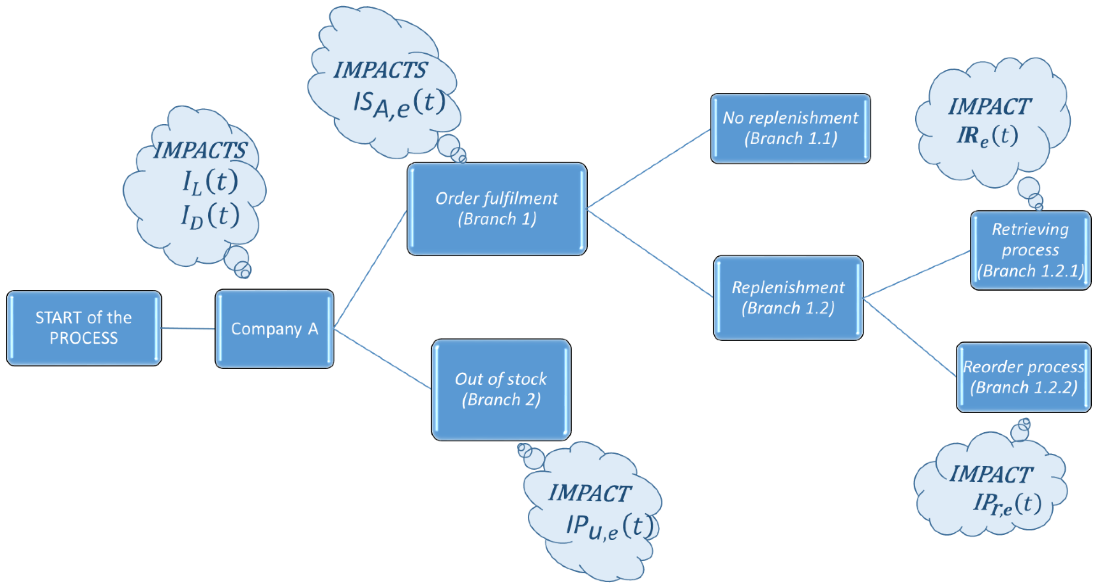
Start of the process. At time , Company A receives orders from its customers and checks whether the amount of orders received can be fulfilled exploiting the “physical” stock of assets. If the stock is sufficient (i.e., ), Company A will follow the order fulfilment process (Branch 1); otherwise, it will incur an out-of-stock situation (Branch 2).
Branch 1—order fulfilment. To fulfil the request, Company A will prepare the order, load the trucks and ship the pallets to its customers. This causes emissions in the environment, which depend on the type of truck used and on its saturation level. Indeed, it can always happen that the 33-pallet lorry used for shipping is not fully saturated (LF < 100%). Infras [46] estimates that the fuel consumption and therefore the emissions of an empty () truck of gross weight 24–40 tons account for approx. 61% of those of a full load () truck. For intermediate values of LF, the impact of a truck can be estimated using Equation (1):
where indicates the amount of emissions type e of a full load truck [47]. To calculate the saturation and the emissions of the trucks used to ship the SKUs to the delivery points, the number of vehicles required for shipment at customer , should be first estimated; the following equation can be used:
where is a fixed quantity describing the amount of palletised SKUs that can be loaded on a 33-pallet truck during shipping. Obviously, the result of Equation (2) should be rounded up to the next whole number; for example, a result of 1.76 means that 2 trucks are required for the shipment. The average saturation of the trucks used for shipment at customer at time , , is computed starting from the total amount of pallets loaded on a truck of given capacity and from the number of pallets shipped, as follows:
The unitary emission type e of truck during shipping at customer , can be computed as follows:
The overall emissions type e of a shipment at time is finally obtained by adding up the contribution of each truck and taking into account the transport distance, as follows:
Further emissions relating to the shipment activities are due to the quota of assets lost and damaged, which, as mentioned, can be considered in the same way as wasted pallets. At day , their environmental impacts, in terms of CO2 emissions, can be calculated as follows:
Product shipment causes the update of the assets inventory at Company A, which will then check whether the stock is lower than OP. If , Company A will not need to replenish its stock of assets (Branch 1.1); otherwise, it will follow the replenishment procedure (Branch 1.2).
Branch 1.1—no replenishment. If the stock of pallets is not replenished, there are no transport activities and therefore the emissions associated with this branch score zero.
Branch 1.2—asset replenishment. If Company A needs to replenish its stock of pallets, transport activities are required, because of either retrieving operations or regular orders. To be more precise, in the case that one (or more) customers own more than MPQ assets in its stock, the Company will start the retrieving process (Branch 1.2.1); otherwise, it will order new assets (Branch 1.2.2).
Branch 1.2.1—retrieving process. Once the customer from which empty assets should be retrieved has been chosen, Company A should estimate the number of vehicles needed for retrieving (), their and their emissions. The former is computed applying the following expression:
where is a fixed quantity describing the amount of empty pallets that can be loaded on a 33-pallet lorry (i.e., 500 pallets). Again, the result of Equation (8) should be rounded up to the next whole number. The average saturation of the trucks used in the retrieving process can be derived starting from the amount of pallets loaded on each truck and the amount of pallets recovered, as follows:
The unitary emission type e of truck during retrieving operations can be finally computed as follows:
The emission type e of all the trucks used to retrieve the pallets from customer at time is finally obtained by adding up the contribution of each truck and taking into account the transport distance, as follows:
Branch 1.2.2—reorder process. In line with the EOQ policy, the amount of new pallets purchased by means of a regular order is fixed and accounts for , which reflect the maximum number of empty pallets that can be loaded on a 33-pallet lorry. Therefore, always score 100% and always score 1 in this process. The amount of emissions of type e generated by a regular order at time thus accounts for
Branch 2—out-of-stock. In the case , Company A will incur an out-of-stock situation and will place a urgent order to the pallet provider. In line with the aim of minimizing the environmental impact of the CLSC, in the model it is assumed that , meaning that whenever an urgent order is required, the transport will be a full truck load. This is expected to decrease the number of transports required and consequently their environmental impact. Hence, as per branch 1.2.2, in this process and always score 100% and 1 respectively. The amount of emissions of type e caused by an urgent order at time thus accounts for:
Figure 1 summarizes the environmental impacts generated in each branch of the decision process.
4.2. Environmental Key Performance Indicators
The following key performance indicators (KPIs), averaged on , are used to assess the environmental performance of the CLSC.
- (1)
- Total impact of retrieving for emissions of type e :
- (2)
- Total impact of shipments for emissions of type e :
- (3)
- Total impact of purchase for emissions of type e :
- (4)
- Total impact of lost and damaged pallets :
- (5)
- Total environmental impact of the CLSC for emissions of type e (, computed by adding up the contributions listed above, as follows:
4.3. Strategic and Economic Performance
Besides the environmental performance, some further economic and strategic KPIs were to assess the efficiency of the asset management process of Company A. Such KPIs reflect those already detailed in Bottani et al. [25]; hence, in the following paragraphs we simply define them, without proposing a detailed computational procedure, which can be found in the previous paper.
The main economic performance of the CLSC is the total cost Company A incurs in managing the flow of assets. For the CLSC considered, takes into account the cost of retrieving assets from the delivery points, the cost of purchasing new assets (by means of regular or urgent orders), the cost of holding the stock of assets and the opportunity cost. Although the economic performance is not the main focus of this study, from a strategic point of view computing allows the observation of how the cost of the CLSC varies when trying to optimize its environmental impact.
Further strategic KPIs considered are:
- (1)
- The amount of proprietary assets , which reflects the average number of pallets owned by Company A and is expressed in (pallets);
- (2)
- Asset rotation , i.e., the number of times per year that the pallet stock rotates. It is expressed in (year−1);
- (3)
- Pallet utilization rate , computed as the ratio between the time (days) of real usage of the asset in the CLSC, either at the delivery point or in transportation activities, and its cycle time (days), which measures the time required for an asset to complete a cycle in the CLSC considered (i.e., from Company A to the customer and back to Company A);
- (4)
- Out of stock , which provides a quantitative measure of those critical situations where Company A does not have pallets available to ship products to its customer (days/year).
4.4. Input Data
To apply the model described in the previous sub-sections, several input data were collected, by means of the direct examination of Company A and from other available sources. The full list of input data is provided in Table 3.
4.5. Software Implementation
The set of equations described in Section 4.1, Section 4.2 and Section 4.3 was implemented in a Microsoft Excel™ simulation model, which consists of two spreadsheets. The first one is the complete database of the inbound/outbound flows of assets recorded by Company A in 2016, including the forward shipments to the customers and the reverse flows of the assets returned. In this spreadsheet, the environmental impacts of the retrieving process are also computed (Equations (8)–(11)). The second spreadsheet reproduces the flow of assets in the CLSC and computes the environmental impacts of shipments, purchases and losses/damages of assets (Equations (1)–(7), (12) and (13)). In the same spreadsheet, the KPIs related to the environmental performance of Company A (Equations (14)–(18)) and the economic/strategic KPIs are also calculated. As far as the OP and MPQ parameters are concerned, simulation was used to vary them in a range of suitable values (from 50 to 1200, step 5) to determine the setting that optimizes the overall performance of the CLSC.
5. Optimization and Ranking Procedures
5.1. Optimization Procedure
As already mentioned, the system under examination generates emissions because of transport activities from Company A to its customers (shipments), from the pallet provider to Company A (regular order or urgent order) and from the customers to Company A (retrieving); a further environmental burden is caused by the amount of assets lost or damaged. A multi-objective optimization procedure was set up using the commercial software ModeFRONTIER™ release 4.6.2 (Esteco S.p.A.), to:
- minimize the emissions of the system;
- minimize the occurrence of out-of-stock situations;
- maximize the use of assets;
- maximize the number of rotations of assets.
As far as the emissions are concerned, the CO2 emissions (i.e., ) are set as the KPI to be minimized, for simplicity; therefore, the results reported in section 6.1 refer to this specific KPI. Nonetheless, minimizing the CO2 emissions is expected to lead to the minimization of the whole environmental impact of the system (i.e., of NOx and SOx emissions too), as the computational procedure is the same for the three types of emissions. Therefore, NOx and SOx emissions are likely to exhibit the same trend as the CO2 emissions.
ModeFRONTIER™ was integrated with the Microsoft Excel™ simulation model, by setting the input data in Table 3 and defining the range for the OP and MPQ variables. A constraint on the maximum number of proprietary pallets () was introduced in the simulation, to take into account the fixed storage capacity of Company A. The solutions returned by ModeFRONTIER™ are marked as “feasible” (green dots in Figure 2, Figure 3, Figure 4 and Figure 5) if they satisfy this constraint and “unfeasible” (yellow dots) otherwise. Finally, only integer values were allowed for , OP and MPQ.
According to the list proposed above, the main outputs returned by the simulation are , , and . Further outcomes provided are , and ; however, these KPIs are not taken into account in the optimization procedure, because the Company has a limited control over them. In fact, depends only on the demand for finished products and therefore cannot be modified by Company A; similarly, depends on the percentage of assets lost or damaged by the customers, over which Company A has no control. , instead, is not taken into account in the optimization procedure because it has a very low value compared to the remaining environmental KPIs (as it will be shown later in the paper); minimizing this component would not lead to significant savings in the environmental emissions of the system.
A two-stage optimization procedure was implemented on ModeFRONTIER™; that procedure consists in the preliminary application of the Design of Experiments (DOE) technique and then in the use of a genetic algorithm. To be more precise, in the DOE stage only the boundary values and the intermediate value of OP and MPQ (i.e., 50, 625 and 1200) were considered, resulting in a 32 full factorial design. Outcomes of the DOE provided some preliminary insights about the solution space and were used to guide the non-dominated sorting genetic algorithm (NSGA-II) towards the optimal solution in the second stage of the optimization. The NSGA-II was selected after a preliminary testing of two additional algorithms, i.e., the multi-objective genetic algorithm (MOGA) and real-coded multi-objective genetic algorithm (ARMOGA). The preliminary testing showed that the NSGA-II was more effective than the remaining algorithms with respect to the computational time, as it explored a lower number of solutions (261 vs. more than 900), without a significant difference in the results returned. This is consonant with the better performance of the NSGA-II in converging near the true Pareto-optimal front compared to other evolutionary algorithms [48]. Overall, the number of configurations simulated is 270 per scenario, which is significantly less than the number of simulations required if the model was simply run under Microsoft Excel™ by varying the OP and MPQ in their range of values (i.e., simulations).
The optimization procedure was run on an Intel® Xeon®E3, 16 GB RAM desktop equipped with Windows 7 Professional. Simulating each scenario (with = 20,000) required approximately 1 h and 2 min.
5.2. Ranking Procedure
As a last step, the multi-criteria decision making (MCDM) tool of ModeFRONTIER™ was exploited to rank the feasible configurations on the basis of their score against the objectives set in the optimization, to enable an effective final choice of the dyad MPQ-OP which returned the best solutions in terms of all the relevant KPIs. A linear MCMD model was chosen to rank the configurations, as it is the simplest approach to ranking. This approach computes a sort of weighted sum of the scores of each KPI subject to optimization, after the user has set a relative importance (weight) for the KPIs. In the “base” configuration, the highest relative importance was assigned to the total CO2 emissions (0.40), in line with the focus of the study, and to the (0.40), because configurations that avoid the occurrence of out-of-stock situations should be preferred for a practical implementation at Company A. The lowest weights (0.10) were assigned to and .
However, because determining the relative importance of the KPIs is a subjective process, two additional scenarios were analyzed in a sensitivity analysis, with different weights assigned to the KPIs. The weights set in these scenarios are:
- 0.25 for all the KPIs. This scenario should capture the situation where Company A attributes the same importance to all KPIs considered in the optimization;
- 0.40 for and and 0.10 for the total environmental impact and for the . This scenario should capture the situation where Company A attributes the highest importance to the strategic KPIs, while the environmental impact is perceived as less important.
6. Results
6.1. Simulation Results
The main results of the simulation runs are reported in the form of trend of the KPIs chosen for the optimization as a function of two problem variables, i.e., OP and MPQ. Such representation is effective in highlighting the impact of these parameters on the environmental performance of the system. A correlation analysis on the simulation outcomes was also performed to help identify relationships among the variables and the KPIs.
The trends of , , and as a function of OP and MPQ are proposed in Figure 2, Figure 3, Figure 4 and Figure 5.
Starting from the environmental KPI, from Figure 2a it can be seen that varies approximately from 75 to 150 kg CO2 eq./day, while solutions with kg CO2 eq./day are all unfeasible. The design space includes (feasible) solutions with the same (e.g., 75 kg CO2 eq./day), which stem from very different values of OP (from 150 up to 1200 pallets). Similarly, the same value of OP (e.g., 150 or 450 pallets) generates very different . Therefore, the relationships between these parameters are not immediately easy to identify. The correlation analysis confirms this consideration: indeed, the correlation between OP and is very weak (0.09). Figure 2b shows, instead, a clear relationship between and MPQ. More precisely, the increase in MPQ involves a corresponding decrease in , which is confirmed by the quite strong negative correlation (−0.68) between these variables. When MPQ is higher, Company A will use recovery operations less frequently, resulting in lower CO2 emissions of the retrieving activities and in a better environmental performance.
With respect to the strategic KPIs, Figure 3a shows that the highest (>200 rotations/year) is obtained with OP ≈ 150–200 pallets. Solutions with OP < 100 pallets are almost all unfeasible. In general, it is reasonable to expect that the increase in OP involves a corresponding increase in the number of . This, in turn, increases the cycle time of assets, worsening the . This is confirmed by the negative correlation between these variables (−0.66). The relationship between and MPQ (Figure 3b) is very similar (−0.49). When the MPQ is higher, Company A will reduce the recovery operations and will probably increase the number of orders, resulting in a higher and thus decreasing the usage of each asset.
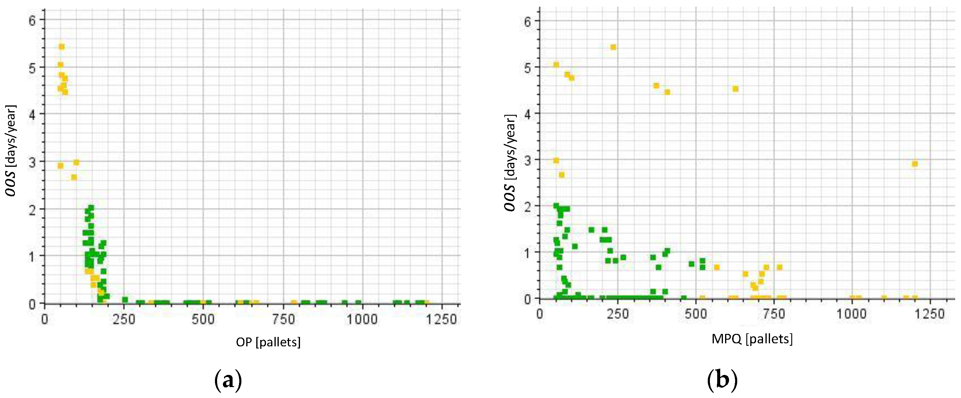
The relationship between and OP is evident from Figure 4a and quite easy to explain. Higher OP generates higher inventory available when orders are placed and therefore, out-of-stock situations are less likely to occur. Accordingly, these variables exhibit a negative correlation (−0.59). From Figure 4a it can also be seen that configurations with OP > 250 pallets always generate null (or almost null) , which is an important evidence for Company A. Conversely, with values of OP from 100 to 200 pallets situations are particularly likely to occur, although the resulting configurations are unfeasible. The relationship between and MPQ is slightly less evident (Figure 4b). In general, lower MPQ seems to generate higher , probably because higher MPQ involves a higher , thus making situations less likely to occur. Nonetheless, it should also be noted that, in feasible configurations, stock-out situations are very unlikely to occur, as their maximum value is 2 days/year. The low correlation coefficient (−0.14) confirms a weak relationship between these variables.
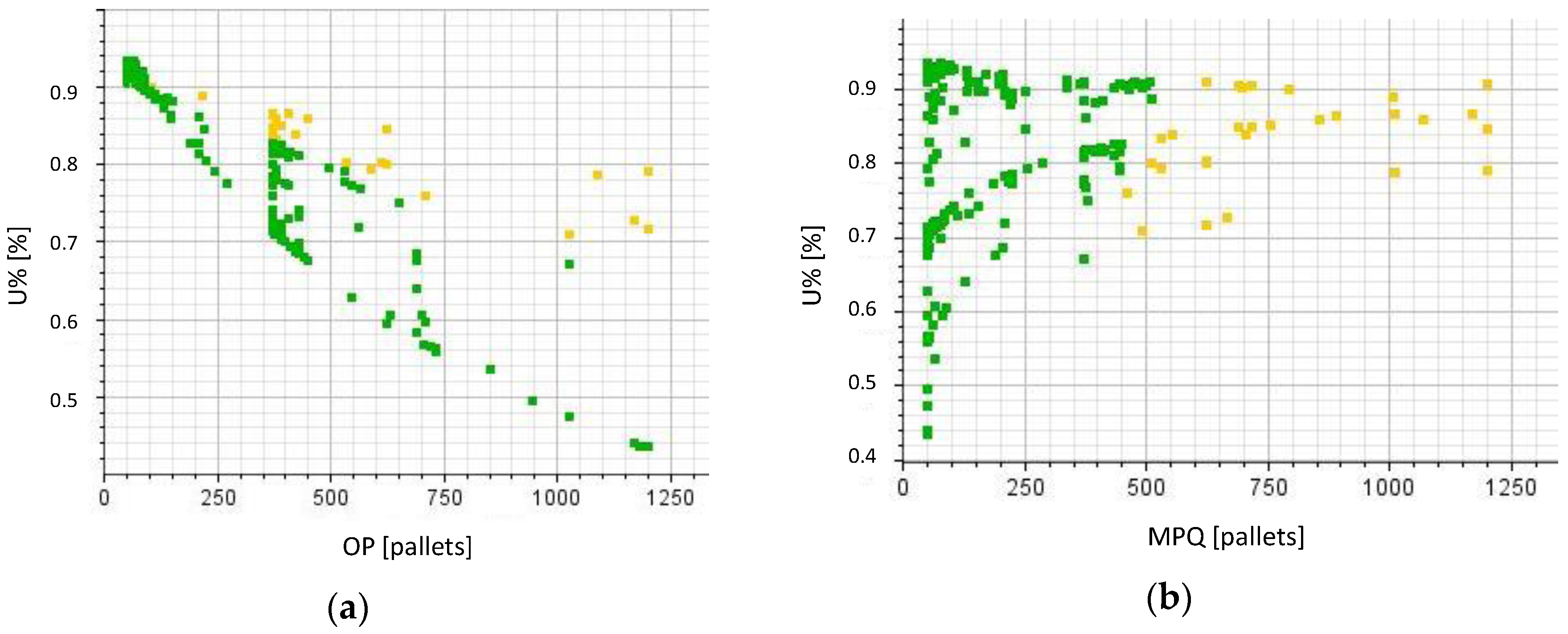
Figure 5a shows that tends to decrease with the increase in OP. Increasing OP causes a corresponding increase in the number of and, consequently, a higher cycle time of assets. Since is inversely proportional to the cycle time, it decreases accordingly. The two variables thus exhibit a strong negative correlation (−0.81). Conversely, the relationship between and MPQ (Figure 5b) seems to be opposite, i.e., the increase in MPQ involves a corresponding increase in . However, this relationship is weaker than the previous one (0.31).
6.2. Multi-Criteria Ranking
The solutions described in the previous paragraph were subject to multi-criteria ranking using the linear MCDM tool of ModeFRONTIER™. We start by considering the “base” scenario, in which the highest importance (0.4) is assigned to the environmental KPI and the , while the importance of the remaining KPIs is set at 0.1. Table 4 shows an extract of the top-5 simulation runs after ranking.
From Table 4 it is easy to see that the top-5 configurations are similar in terms of all environmental emissions (, and ), which confirms that these KPIs follow the same trend. , which was subject to minimization, turns out to be in the range 75.50 to 76.43 kg CO2 eq./day. It is also easy to see that, as already recalled, does not vary as a function of OP and MPQ, as it depends only on the amount of pallets lost and damaged. Such contribution accounts for approximately 38.28% of the total CO2 emission of Company A. does not vary either, as shipments are triggered by the customers’ demand and as such do not depend on OP and MPQ.
In all the top-5 configurations, is almost constant; for instance, always accounts for 0.23 kg CO2/day, corresponding to approximately 0.30% of the total CO2 emissions of the system. and account, instead, for approximately 0.50% of and , respectively. Therefore, purchasing activities have very limited impact on the environmental performance of the CLSC. The last environmental KPIs, i.e., , turns out to be the most important quota of the environmental emissions of the CLSC. To be more precise, ranges from 42.76 to 43.69 kg CO2 eq./day, corresponding to 56–57% of ; the contribution of and to and is even higher (ca. 91%). This suggests that minimizing basically corresponds to minimizing for the system considered.
With respect to the strategic KPIs, the top-5 configurations do not exhibit a significant difference in terms of , which accounts for 0.15 days/year in the first two configurations and is null in the remaining ones. Despite an greater than 0, the first ranked configuration, obtained setting OP = 175 and MPQ = 360 pallets, shows a very high and a good . Configurations 196, 237 and 170 are instead interesting because of the null , which could be of practical interest to Company A; however, and are slightly worse compared to the first two ranked configuration.
6.3. Sensitivity Analysis
We now consider the case of a change in the relative importance of the KPIs subject to optimization, to highlight possible modifications in the asset management strategy of Company A as a function of the weights assigned to these KPIs.
We begin by analyzing the situation in which the same relative importance (i.e., 0.25) is assigned to all the KPIs subject to optimization; with these weights, the top-5 configurations resulting after ranking are proposed in Table 5. As Table 5 shows, in the case all the KPIs are given the same importance, the results are quite variable in terms of the total environmental emissions (, and ), and . Moreover, the top-5 configurations all exhibit a non-null , meaning that if Company A is interested in enhancing also and , the occurrence of stock-out situations cannot be avoided. Looking, for instance, at the CO2 emissions (), it can be noticed that they are significantly higher in this scenario than in the “base” scenario, with a peak of 102.6 kg CO2 eq./day in the third ranked configuration. Once again, this is due to the relevant contribution of . and improve significantly compared to the “base” scenario, reaching ca. 150 rotations/year and 88.3% respectively in the first ranked configuration.
It is interesting to note that configuration 154 ranked fourth in this scenario and first in the “base” scenario; this suggests that this configuration returns performance values that are quite robust with respect to the weights assigned to the KPIs.
A further interesting point is that, apart from configuration 154, all the remaining configurations are obtained setting a quite low MPQ (from 120 to 265 pallets). Because of the low MPQ, from a practical point of view it could be hypothesized that Company A would be able to carry out retrieving operations using low capacity vehicles. These vehicles produce less CO2 compared to 33-pallet lorries (whose use has been hypothesized in this study); therefore, the real environmental impact could be lower than that estimated by our model.
Table 6 shows the results obtained in the case the highest importance (0.4) is assigned to and , while less importance (0.1) is assigned to and . As it is reasonable to expect, the top-5 configurations all exhibit a very good (around 200 rotations/year), which involves a limited amount of proprietary assets (ca. 1000 pallets at maximum). The environmental emissions in this situation are not optimized, because, with fewer pallets, Company A should organize very frequent collections of pallets from the customers’ sites. Nonetheless, as per the previous case, the MPQ of the top ranked configurations is quite low, which suggests that Company A could carry out retrieving operations using low capacity vehicles, resulting in reduced CO2 emissions compared to those computed using our model. Finally, the results in Table 6 confirm that when maximizing and , out-of-stock situations are more likely to occur.
7. Conclusions
This paper has proposed an analysis of the environmental emissions caused by the asset management process of a real CLSC, consisting of a pallet provider, a manufacturer (Company A) and several retailers. The analysis was supported by a Microsoft Excel™ model, which computes the CO2, NOx and SOx emissions of the system on the basis of the flows of asset. This model was integrated with ModeFRONTIER™ in a multi-objective optimization procedure, which took into account these emissions and some strategic KPIs of Company A. The multi-objective optimization targeted, in particular, the minimization of the CO2 emissions, coupled with the minimization of stock-out occurrence and the maximization of assets usage and rotation. As a result, the setting of the asset management process, in terms of OP and MPQ, which performed best against the objectives set was derived as a function of the relative importance assigned to each KPI.
When assigning the highest relative importance to the minimization of CO2 emissions and occurrence (“base” scenario), the best performance of the system is achieved setting OP = 175 and MPQ = 360 pallets. With this setting, the total CO2 emission of the CLSC accounts for 75.50 kg CO2 eq./day approximately. The different components of the environmental impact contribute to this KPI in different ways and to a different extent. Asset retrieving activities contribute to the total impact to the greatest extent (approx. 42.76 kg CO2/day), while the CO2 emissions caused by the purchasing of new assets and the replenishment of lost and damaged assets are significantly less relevant. The CO2 emissions due to the shipping activities, although not irrelevant, cannot be minimized by Company A, as shipments depend on the final customers’ demand only. This implicitly means that to minimize the total emissions of the system, Company A should actually minimize the environmental burdens caused by asset retrieving operations. In turn, the high environmental impact of retrieving activities is due to the quite relevant distance between Company A and its customers (delivery points), which is always higher than 250 km (approximately 496 km on average) in the system considered. This distance also prevents the possibility of visiting more than one customer in a single shipment. Moreover, as retrieving activities are ad hoc transports, they are rarely optimized in terms of truck load. Therefore, if using lorries with a capacity of 33 pallets, an effective strategy to decrease the environmental impact of retrieving operations is to set the MPQ at a quite high value, close to a full truck load shipment—this is why the top-5 ranked configurations of the “base” scenario all exhibit MPQ > 360 pallets.
Besides the “base” scenario, we carried out a sensitivity analysis to evaluate two additional situations, in which different weights were set for the KPIs subject to optimization. In the first situation, the same relative importance was assigned to all KPIs considered in the optimization process. In this case, the most effective performance is obtained when setting OP = 145 and MPQ = 215 pallets and exhibits a very good and . However, the environmental impact of the CLSC is not optimized in this scenario and stock-out situations are more likely to occur. In the case where the highest importance is assigned to and , the top ranked configurations obviously show excellent scores against these KPIs, while the environmental performance and the worsen significantly compared to the base scenario. Nonetheless, it is interesting to note that the MPQ of the top-ranked configurations examined in the sensitivity analysis is always lower than that of the base scenario and, in particular, it is lower than the number of assets that can be retrieved with a full-truck load shipment. From a practical perspective, this means that retrieving activities will be more frequent, but that Company A could carry out these activities using low capacity vehicles (instead of 33-pallet lorries, as hypothesized in our model); therefore, the is room for reducing the resulting environmental impact.
A further consideration that can be derived from the analysis of the top-5 ranked configurations of all scenarios is that the total environmental performance and the total cost of the CLSC, although not strictly proportional, seem to go at the same pace. The lowest total environmental impact and total cost were indeed obtained in the first scenario (i.e., when the minimization of the environmental KPI is given the highest relative importance), while, with the increase in the total impact, the total cost of the system increases too.
To sum up, the results of this study provide Company A with an overview of its current performance in terms of environmental emissions and can help the company improve the environmental impact of its asset management process.
From a theoretical perspective, the model developed in this paper includes a set of formulae that were added an original (economic) model for the computation of the environmental emissions of the system. From a practical perspective, this paper is structured as a case study, as it focuses on the specific context of Company A. Nonetheless, a similar evaluation can be easily extended to different companies or CLSCs. When analyzing different systems, it could be interesting to evaluate whether lower distances between the focal company and its customers could modify the environmental balance of the system or change the strategy to be adopted for assets management. Similarly, the multi-objective optimization procedure could be applied with different relative importance of the KPIs or setting different objectives, with the aim to evaluate the impact of different assets management strategies on the environmental performance of the system. Therefore, the model itself represents an interesting addition to the literature about CLSCs.
Acknowledgments
This research was supported by the research Grant No. D92I15000210008 (project code RBSI14L97M), called “ESCALATE—Economic and Environmental Sustainability of Supply Chain and Logistics with Advanced Technologies”, funded by the Italian Ministry of University and Research under the SIR (Scientific Independence of young Researchers) 2014 program (decree of 23 January 2014, No. 197) and awarded to the first author.
Author Contributions
Eleonora Bottani acted as the coordinator of this study and was in charge of the general design of the research activities, assembly and review of the related material. Giorgia Casella developed the model, carried out the simulation analyses and the multi-objective optimization. The paper was written together by all of the authors.
Conflicts of Interest
The authors declare no conflict of interest. The founding sponsors had no role in the design of the study; in the collection, analyses or interpretation of data; in the writing of the manuscript; nor in the decision to publish the results.
References
- Guide, V.-R.J.; van Wassenhove, L.-N. The evolution of closed-loop supply chain research. Oper. Res. 2009, 57, 10–18. [Google Scholar] [CrossRef]
- Govindan, K.; Soleimani, H.; Kannan, D. Reverse logistics and closed-loop supply chain: A comprehensive review. Eur. J. Oper. Res. 2015, 240, 603–626. [Google Scholar] [CrossRef] [Green Version]
- Badurdeen, F.; Iyengar, D.; Goldsby, T.; Metta, H.; Gupta, S.; Jawahir, I. Extending total life-cycle thinking to sustainable supply chain design. Int. J. Prod. Lifecycle Manag. 2009, 4, 49–67. [Google Scholar] [CrossRef]
- Guide, V., Jr.; Jayaraman, V.; Linton, J. Building contingency planning for closed-loop supply chains with product recovery. J. Oper. Manag. 2003, 21, 259–279. [Google Scholar] [CrossRef]
- Dekker, R.; Inderfurth, K.; van Wassenhove, L.; Fleischmann, M. Reverse Logistics—Quantitative Models for Closed-Loop Supply Chains; Springer: Berlin, Germany, 2004. [Google Scholar]
- Flapper, S.; van Nunen, J.; van Wassenhove, L. Managing Closed-Loop Supply Chains; Springer: Berlin, Germany, 2005. [Google Scholar]
- Tibben-Lembke, R. Strategic use of the secondary market for retail consumer goods. Calif. Manag. Rev. 2004, 46, 90–104. [Google Scholar] [CrossRef]
- Jena, S.; Sarmah, S. Future aspect of acquisition management in closed-loop supply chain. Int. J. Sustain. Eng. 2016, 9, 266–276. [Google Scholar] [CrossRef]
- European Commission. BRIGDE WP09—Returnable Transport Items: The market for EPCglobal applications. 2007. Available online: HTTP://BRIDGE-PROJECT.EU/DATA/FILE/BRIDGE%20WP09%20RETURNABLE%20ASSETS%20MARKET%20ANALYSIS.PDF (accessed on 26 October 2016).
- ISO/IEC. ISO/IEC 15459-5: 2014 Information Technology—Automatic Identification and Data Capture Techniques—Unique Identification—Part 5: Individual Returnable Transport Items (RTIs). 2014. Available online: HTTP://WWW.ISO.ORG/ISO/HOME/STORE/CATALOGUE_ICS/CATALOGUE_DETAIL_ICS.HTM?CSNUMBER=54785 (accessed on 26 October 2016).
- Johansson, O.; Hellstrom, D. The effect of asset visibility on managing returnable transport items. Int. J. Phys. Distrib. Logist. Manag. 2007, 37, 799–815. [Google Scholar] [CrossRef]
- Alfonso-Lizarazo, E.; Montoya-Torres, J.; Gutiérrez-Franco, E. Modeling reverse logistics process in the agro-industrial sector: The case of the palm oil supply chain. Appl. Math. Model. 2013, 37, 9652–9664. [Google Scholar] [CrossRef]
- Kroon, L.; Vrijens, G. Returnable containers: An example of reverse logistics. Int. J. Phys. Distrib. Logist. Manag. 1995, 25, 56–68. [Google Scholar] [CrossRef] [Green Version]
- Carrasco-Gallego, R.; Ponce-Cueto, E.; Dekker, R. Closed-loop supply chains of reusable articles: A typology grounded on case studies. Int. J. Prod. Res. 2012, 50, 5582–5596. [Google Scholar] [CrossRef]
- Wang, Z.; Soleimani, H.; Kannan, D.; Xu, L. Advanced cross-entropy in closed-loop supply chain planning. J. Clean. Prod. 2016, 135, 201–213. [Google Scholar] [CrossRef]
- Xu, H.; Cao, E. Closed-loop supply chain network equilibrium model and its Newton method. Kybernetes 2016, 45, 393–410. [Google Scholar] [CrossRef]
- Wu, C.; Barnes, D. Partner selection for reverse logistics centres in green supply chains: A fuzzy artificial immune optimisation approach. Prod. Plan. Control. 2016, 27, 1356–1372. [Google Scholar] [CrossRef]
- Zhu, Q.; Sarkis, J.; Lai, K. Green supply chain management implications for ‘closing the loop’. Transp. Res. 2008, 44, 1–18. [Google Scholar] [CrossRef]
- Preuss, L. The Green Multiplier: A Study of Environmental Protection and the Supply Chain; Palgrave MacMillan: Basingstoke, UK, 2005. [Google Scholar]
- Kannan, G.; Noorul Haq, A.; Devika, M. Analysis of closed loop supply chain using genetic algorithm and particle swarm optimisation. Int. J. Prod. Res. 2009, 47, 1175–1200. [Google Scholar] [CrossRef]
- Rogers, D.; Tibben-Lembke, R. An examination of reverse logistics practices. J. Bus. Logist. 2001, 22, 129–148. [Google Scholar] [CrossRef]
- Stock, J.; Speh, T.; Shear, H. Many happy (product) returns. Harv. Bus. Rev. 2002, 80, 16–17. [Google Scholar]
- Sbihi, A.; Eglese, R. Combinatorial optimization and Green Logistics. 4OR A Q. J. Oper. Res. 2007, 5, 99–116. [Google Scholar] [CrossRef] [Green Version]
- Lambert, S.; Riopel, D.; Abdul-Kader, W. A reverse logistics decisions conceptual framework. Comput. Ind. Eng. 2011, 61, 561–581. [Google Scholar] [CrossRef]
- Bottani, E.; Montanari, R.; Rinaldi, M.; Vignali, G. Modeling and multi-objective optimization of closed loop supply chains: A case study. Comput. Ind. Eng. 2015, 87, 328–342. [Google Scholar] [CrossRef]
- Chen, A.; Wang, X.-P.; Chen, B.-J.; Li, W.-W. Research on methods of reverse logistic vendor selection under closed-loop supply chain. In Proceedings of the 14th International Conference on Management Science and Engineering (ICMSE07), Harbin, China, 20–22 August 2007; pp. 879–884. [Google Scholar]
- Ismail, M.; Ainaa, S.; Abdullah, Z.; Shaharudin, M.; Zailani, S. A reputation-based strategy towards sustainable services by third party logistics (3PLs) in closed-loop supply chains (CLSCs). In Proceedings of the 2nd International Symposium on Technology Management and Emerging Technologies (ISTMET 2015), Langkawi, Malaysia, 25–27 August 2015; pp. 442–447. [Google Scholar]
- Gallo, M.; Murino, T.; Santillo, L. Evaluating the impact of product eco-redesign on CLSC performances through a system dynamics approach. Int. J. Prod. Qual. Manag. 2016, 18, 191–209. [Google Scholar] [CrossRef]
- Talbot, S.; Lefebvre, E.; Lefebvre, L. Closed-loop supply chain activities and derived benefits in manufacturing SMEs. J. Manuf. Technol. Manag. 2007, 18, 627–658. [Google Scholar] [CrossRef]
- Georgiadis, P.; Besiou, M. Environmental and economical sustainability of WEEE closed-loop supply chains with recycling: A system dynamics analysis. Int. J. Adv. Manuf. Technol. 2010, 47, 475–493. [Google Scholar] [CrossRef]
- Gao, N.; Ryan, S. Closed-loop supply chain network design under carbon emission regulations. In Proceedings of the 61st Annual IIE Conference and Expo, Reno, NV, USA, 21–25 May 2011; pp. 3367–3374. [Google Scholar]
- Shi, W.; Min, K. A study of product weight and collection rate in closed-loop supply chains with recycling. IEEE Trans. Eng. Manag. 2013, 60, 409–423. [Google Scholar] [CrossRef]
- Hasanov, P.; Jaber, M.; Zanoni, S.; Zavanella, L. Closed-loop supply chain system with energy, transportation and waste disposal costs. Int. J. Sustain. Eng. 2013, 6, 352–358. [Google Scholar] [CrossRef]
- Chen, Y.; Wang, L.-C.; Chen, T.-L.; Wang, A.; Cheng, C.-Y. A multi-objective model for solar industry closed-loop supply chain by using particle swarm optimization. In Proceedings of the 24th International Conference on Flexible Automation and Intelligent Manufacturing (FAIM 2014), San Antonio, TX, USA, 20–23 May 2014; DEStech Publications, Inc.: Lancaster, PA, USA; pp. 459–466. [Google Scholar]
- Chen, Y.; Chan, F.; Chung, S. An integrated closed-loop supply chain model with location allocation problem and product recycling decisions. Int. J. Prod. Res. 2015, 53, 3120–3140. [Google Scholar] [CrossRef]
- Garg, K.; Kannan, D.; Diabat, A.; Jha, P. A multi-criteria optimization approach to manage environmental issues in closed loop supply chain network design. J. Clean. Prod. 2015, 100, 297–314. [Google Scholar] [CrossRef]
- Alimorandi, A.; Yussuf, R.; Ismail, N.; Zulkifli, N. Developing a fuzzy linear programming model for locating recovery facility in a closed loop supply chain. Int. J. Sustain. Eng. 2015, 8, 122–137. [Google Scholar] [CrossRef]
- Govindan, K.; Jha, P.; Garg, K. Product recovery optimization in closed-loop supply chain to improve sustainability in manufacturing. Int. J. Prod. Res. 2016, 54, 1463–1486. [Google Scholar] [CrossRef]
- Dutta, P.; Das, D.; Schultmann, F.; Fröhling, M. Design and planning of a closed-loop supply chain with three way recovery and buy-back offer. J. Clean. Prod. 2016, 135, 604–619. [Google Scholar] [CrossRef]
- Kim, S.H.; Yoon, S.G.; Chae, S.H.; Park, S. Economic and environmental optimization of a multi-site utility network for an industrial complex. J. Environ. Manag. 2010, 91, 690–705. [Google Scholar] [CrossRef] [PubMed]
- Eriksson, E.; Blinge, M.; Lovgren, G. Life cycle assessment of the road transport sector. Sci. Total Environ. 1996, 189/190, 69–76. [Google Scholar] [CrossRef]
- Muncrief, R. NOX Emissions from Heavy-Duty and Light-Duty Diesel Vehicles in the EU: Comparison of Real-World Performance and Current Type-Approval Requirements. 2010. Available online: HTTP://WWW.THEICCT.ORG/SITES/DEFAULT/FILES/PUBLICATIONS/EURO-VI-VERSUS-6_ICCT_BRIEFING_06012017.PDF (accessed on 5 December 2017).
- United States Environmental Protection Agency (EPA). Overview of the Human Health and Environmental Effects of Power Generation: Focus on Sulfur Dioxide (SO2), Nitrogen Oxides (NOx) and Mercury (Hg). 2002. Available online: HTTPS://ARCHIVE.EPA.GOV/CLEARSKIES/WEB/PDF/OVERVIEW.PDF (accessed on 15 January 2018).
- Carraro, A.L.; Thorn, B.K.; Woltag, H. Characterizing the carbon footprint of wood pallet logistics. For. Prod. J. 2014, 64, 232–241. [Google Scholar]
- Harris, F. How many parts to make at once. Prod. Eng. 1913, 10, 135–136. [Google Scholar] [CrossRef]
- Infras. Handbook Emission Factors for Road Transport—HBEFA. 2010. Available online: HTTP://WWW.HBEFA.NET/E/HELP/HBEFA32_HELP_EN.PDF (accessed on 26 October 2016).
- Bertolini, M.; Bottani, E.; Vignali, G.; Volpi, A. Comparative life cycle assessment of packaging systems for extended shelf life milk. Packag. Technol. Sci. 2016, 29, 525–546. [Google Scholar] [CrossRef]
- Deb, K.; Pratap, A.; Agarwal, S. A fast and elitist multi objective genetic algorithm: NSGA-II. IEEE Trans. Evol. Comput. 2002, 6, 182–197. [Google Scholar] [CrossRef]
Figure 1.
Sketch of the model and environmental emissions (adapted from [25]).
Figure 1.
Sketch of the model and environmental emissions (adapted from [25]).

Figure 2.
Trend of [kg CO2 eq./day] as function of OP (a) and MPQ (b).
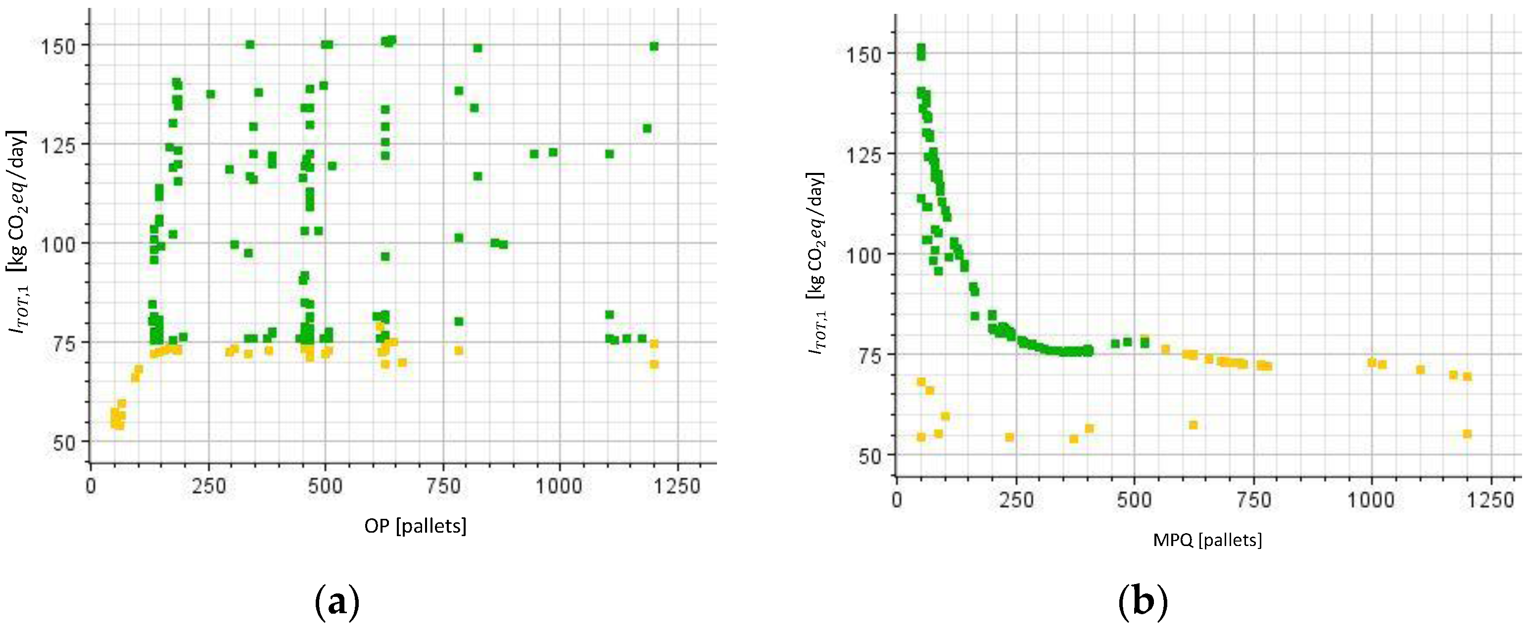
Figure 3.
Trend of [years-1] as function of OP (a) and MPQ (b).
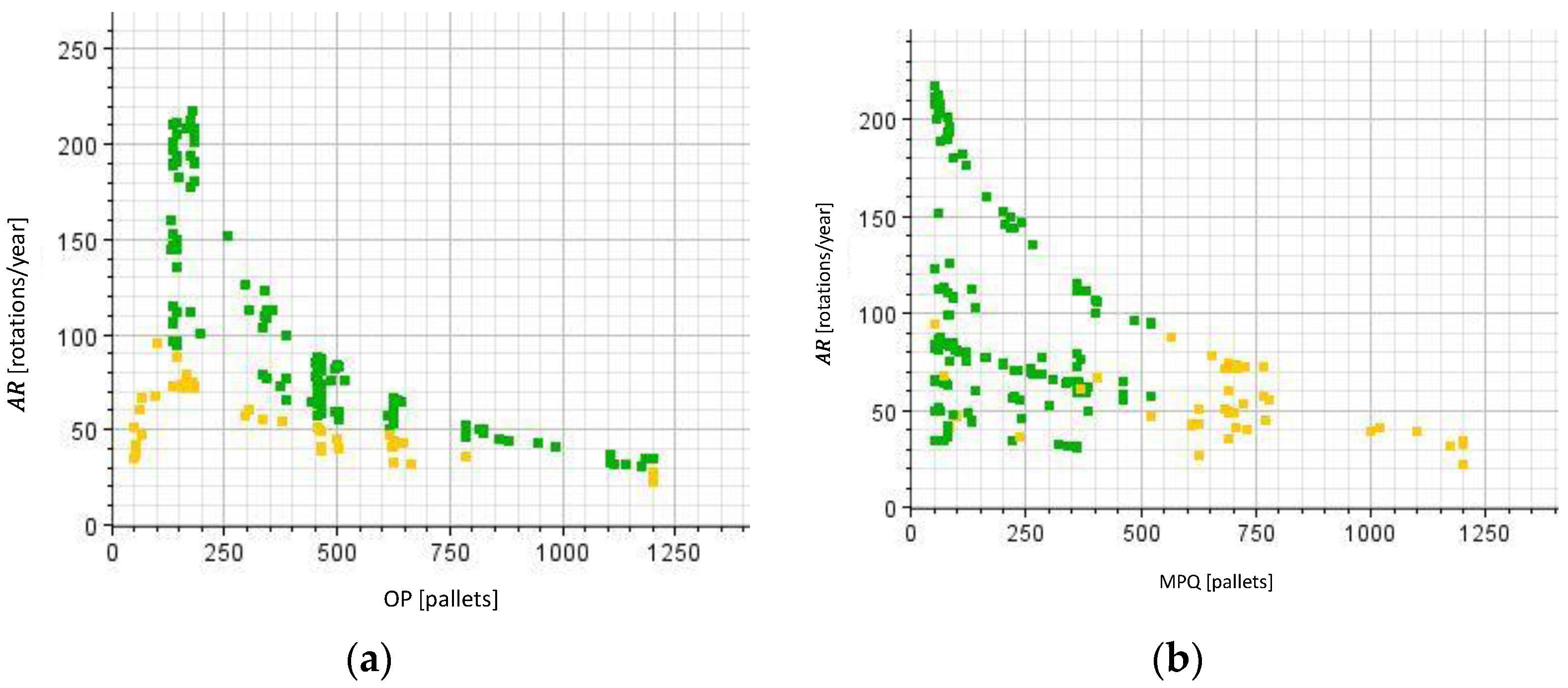
Figure 4.
Trend of [days/year] as function of OP (a) and MPQ (b).

Figure 5.
Trend of [%] as function of OP (a) and MPQ (b).

Table 1.
Closed-loop supply chain (CLSC) models reviewed in this study and contribution of the present study.
Table 1.
Closed-loop supply chain (CLSC) models reviewed in this study and contribution of the present study.
| Paper | Field | Sustainability Perspective | Methodology | Main Results | |
|---|---|---|---|---|---|
| Environmental | Economic | ||||
| Georgiadis and Besiou [30] | Waste of electric and electronic equipment in CLSC | x | x | Extension of a system dynamics-based model | The production of recycled materials of high quality improves the economical sustainability and the availability of natural resources |
| Gao and Ryan [31] | Document-office company operating in the Iberian market | x | x | Network design | Suggestions to balance the trade-offs between usual costs and the impact of carbon emission regulations |
| Shi and Min [32] | Supply chain centralization/decentralization | x | Modelling framework | Evaluation of the impact of supply chain centralization or decentralization strategies and of the relationships between government subsidy and fee on these strategies | |
| Alfonso-Lizarazo et al. [12] | Palm oil CLSC | x | Mathematical model | Impact of the simultaneous analysis of direct and reverse flows on the net economic profit of the CLSC | |
| Hasanov et al. [33] | Economic value and energy content of products | x | Novel modelling framework | Suggestions for a SC model that takes into account energy, transportation and disposal costs | |
| Chen et al. [34] | Crystalline solar energy industry | x | x | Deterministic multi-objective mixed integer programming model | Suggestions for capacity expansion, technology selection, supply chain design, factory location options and capacity allocation |
| Chen et al. [35] | Ink-and-toner cartridge delivering and recycling in Hong Kong | x | Mix integer linear programming model | Suggestion for integration of forward and reverse flows | |
| Garg et al. [36] | Geyser manufacturer CLSC | x | Interactive multi-objective programming approach algorithm | The inflow of returns with better recovery options substantially influences the economic benefit for business by increasing the demand for new products in first customer markets | |
| Alimorandi et al. [37] | CLSC | x | A fuzzy mixed integer linear programming model | Suggestions for a new design of supply chain network in which waste of materials is minimized and the new raw materials are necessary only when the used products may not be recovered | |
| Govindan et al. [38] | Case study from an electrical manufacturing industry | x | x | Multi-objective mixed integer mathematical problem | Suggestions to enhance manufacturing sustainability |
| Bottani et al. [25] | Manufacturer of fast moving consumer goods operating in the North of Italy | x | Mathematical model reproduced on a Microsoft Excel™ simulator | Suggestions for asset management strategies that minimize the total cost of the CLSC | |
| Dutta et al. [39] | CLSC of electronics products category | x | Recovery framework | Considerations about the profitability of the system as a function of the probability of product acceptance. | |
| Present study | Manufacturer of fast moving consumer goods operating in the North of Italy | x | x | Mathematical model reproduced on a Microsoft Excel™ simulator | Suggestions to minimize the environmental impact of the reverse logistics activities of RTI in a CLSC |
Table 2.
Nomenclature (partially taken from Bottani et al. [25], with permission from Elsevier).
Table 2.
Nomenclature (partially taken from Bottani et al. [25], with permission from Elsevier).
| Symbol | Description | Unit of Measurement |
|---|---|---|
| Indexes | ||
| i | delivery point (i = 1, … 7) | - |
| n | truck (n = 1, …ntruck) | - |
| t | simulation day (t = 0, … Ndays) | - |
| e | type of environmental emission (e = 1 for CO2; e = 2 for NOx; e = 3 for SOx) | - |
| Subscripts | ||
| L, D | lost or damaged pallets | - |
| r, s, p_u, p_r | recovery, shipment, urgent purchase, regular purchase | - |
| Tot | Total | - |
| DP | delivery point | - |
| A | Company A | - |
| Prov | pallet provider | - |
| Superscripts | ||
| P | “physical” | - |
| T | “theoretical” | - |
| Simulation parameters | ||
| Ndays | simulation duration | (days) |
| Delivery point parameters | ||
| order issued | (pallets) | |
| amount of assets retrieved | (pallets) | |
| , | percentage of assets lost and damaged | (%) |
| distance between delivery point and Company A | (km) | |
| Company A parameters | ||
| Ndays/year | working days per year | (days) |
| amount of assets shipped to delivery point | (pallets) | |
| , | physical and theoretical stock of assets | (pallets) |
| , | amount of assets purchased through a regular or urgent order | (pallets) |
| amount of proprietary assets | (pallets) | |
| distance from Company A to the pallet provider | (km) | |
| OP | order point | (pallets) |
| MPQ | minimum picked quantity (minimum amount of assets to be collected through retrieving operations) | (pallets) |
| Environmental parameters | ||
| CO2 emissions of a lost/damaged pallet | ||
| LF | load factor of a truck | (%) |
| IFLTe | emissions type e of a full load truck | (/km) |
| Other parameters | ||
| amount of palletized SKUs that can be loaded on a truck during shipment and retrieving | (pallets/truck) |
Table 3.
Input data (partially taken from Bottani et al. [25], with permission from Elsevier).
Table 3.
Input data (partially taken from Bottani et al. [25], with permission from Elsevier).
| Parameter | Numerical Value | Measurement Unit | Source |
|---|---|---|---|
| 260 | (days) | Company A | |
| = | 500 | (pallets) | Company A |
| 2.5% | - | Company A | |
| 1% | - | Company A | |
| 362 (i = 1); 358 (i = 2); 606 (i = 3); 352 (i = 4); 232 (i = 5); 934 (i = 6); 632 (i = 7) | (km) | Company A | |
| 38 | (km) | Company A | |
| 500 | (pallets/truck) | Company A | |
| 33 | (pallets/truck) | Company A | |
| 7.16 | [44] | ||
| 0.699 | (kg /km) | [42] | |
| 0.21 × 10⁻³ | (kg NOx/km) | [42] | |
| 0.08 × 10⁻³ | (kg SOx/km) | [42] |
Table 4.
Top-5 configurations of the “base” scenario after ranking.
| Decision Variables | Strategic KPIs | CO2 eq. (kg/day) | NOx (g/day) | SOx (g/day) | ||||||||||||||||
|---|---|---|---|---|---|---|---|---|---|---|---|---|---|---|---|---|---|---|---|---|
| Configuration ID | OP | MPQ | OOS | AR | U% | PA | ||||||||||||||
| 154 | 175 | 360 | 0.15 | 111.63 | 87.15 | 2047 | 42.76 | 0.23 | 28.90 | 3.61 | 75.50 | 12.80 | 0.07 | 1.08 | 14.00 | 4.80 | 0.03 | 0.14 | 5.33 | 179.28 |
| 262 | 195 | 400 | 0.15 | 100.80 | 86.85 | 2253 | 43.69 | 0.23 | 28.90 | 3.61 | 76.43 | 13.10 | 0.07 | 1.08 | 14.27 | 5.00 | 0.03 | 0.14 | 5.43 | 184.07 |
| 196 | 335 | 360 | 0.00 | 79.372 | 82.78 | 2205 | 43.05 | 0.23 | 28.90 | 3.61 | 75.79 | 12.90 | 0.07 | 1.08 | 14.08 | 4.90 | 0.03 | 0.14 | 5.36 | 184.31 |
| 237 | 345 | 370 | 0.00 | 76.41 | 82.23 | 2262 | 43.07 | 0.23 | 28.90 | 3.61 | 75.81 | 12.90 | 0.07 | 1.08 | 14.09 | 4.90 | 0.03 | 0.14 | 5.36 | 184.47 |
| 170 | 375 | 360 | 0.00 | 73.19 | 81.46 | 2228 | 43.18 | 0.23 | 28.90 | 3.61 | 75.92 | 12.90 | 0.07 | 1.08 | 14.13 | 4.90 | 0.03 | 0.14 | 5.38 | 185.28 |
Table 5.
Top-5 configurations after ranking with modified weights—first scenario.
| Decision Variables | Strategic KPIs | CO2 eq. (kg/day) | NOx (g/day) | SOx (g/day) | ||||||||||||||||
|---|---|---|---|---|---|---|---|---|---|---|---|---|---|---|---|---|---|---|---|---|
| Configuration ID | OP | MPQ | OOS | AR | U% | PA | ||||||||||||||
| 209 | 145 | 215 | 0.82 | 149.79 | 88.29 | 1467 | 48.17 | 0.23 | 28.9 | 3.61 | 80.91 | 14.47 | 0.07 | 1.08 | 15.62 | 5.51 | 0.03 | 0.14 | 5.95 | 202.03 |
| 61 | 145 | 240 | 0.82 | 147.05 | 88.21 | 1500 | 46.69 | 0.23 | 28.9 | 3.61 | 79.43 | 14.02 | 0.07 | 1.08 | 15.18 | 5.34 | 0.03 | 0.14 | 5.78 | 195.72 |
| 246 | 175 | 120 | 0.07 | 177.05 | 84.9 | 972 | 69.32 | 0.23 | 28.9 | 3.61 | 102.06 | 20.83 | 0.07 | 1.08 | 21.97 | 7.93 | 0.03 | 0.14 | 8.37 | 288.01 |
| 154 | 175 | 360 | 0.15 | 111.63 | 87.15 | 2047 | 42.76 | 0.23 | 28.9 | 3.61 | 75.5 | 12.80 | 0.07 | 1.08 | 14.00 | 4.80 | 0.03 | 0.14 | 5.33 | 179.23 |
| 91 | 145 | 265 | 0.89 | 135.51 | 88.19 | 1714 | 44.99 | 0.23 | 28.9 | 3.61 | 77.73 | 13.52 | 0.07 | 1.08 | 14.67 | 0.14 | 0.03 | 0.14 | 5.59 | 188.56 |
Table 6.
Top-5 configurations after ranking with modified weights—second scenario.
| Decision Variables | Strategic KPIs | CO2 eq. (kg/day) | NOx (g/day) | SOx (g/day) | ||||||||||||||||
|---|---|---|---|---|---|---|---|---|---|---|---|---|---|---|---|---|---|---|---|---|
| Configuration ID | OP | MPQ | OOS | AR | U% | PA | ||||||||||||||
| 130 | 135 | 60 | 1.93 | 210.9 | 89.28 | 967 | 70.64 | 0.23 | 28.9 | 3.61 | 103.38 | 21.22 | 0.07 | 1.08 | 22.38 | 8.09 | 0.03 | 0.14 | 8.52 | 299.89 |
| 62 | 145 | 60 | 1.63 | 211.25 | 87.83 | 919 | 79.03 | 0.23 | 28.9 | 3.61 | 111.77 | 23.74 | 0.07 | 1.08 | 24.90 | 9.05 | 0.03 | 0.14 | 9.48 | 335.18 |
| 78 | 135 | 85 | 1.93 | 196.68 | 90.39 | 1051 | 63.12 | 0.23 | 28.9 | 3.61 | 95.86 | 18.96 | 0.07 | 1.08 | 20.12 | 7.22 | 0.03 | 0.14 | 7.66 | 268.14 |
| 123 | 135 | 80 | 1.93 | 200.95 | 88.96 | 1030 | 68.1 | 0.23 | 28.9 | 3.61 | 100.84 | 20.46 | 0.07 | 1.08 | 21.61 | 7.79 | 0.03 | 0.14 | 8.23 | 288.14 |
| 191 | 145 | 50 | 2.01 | 211.93 | 87.7 | 886 | 80.97 | 0.23 | 28.9 | 3.61 | 113.71 | 24.33 | 0.07 | 1.08 | 25.48 | 9.27 | 0.03 | 0.14 | 9.71 | 344.01 |
© 2018 by the authors. Licensee MDPI, Basel, Switzerland. This article is an open access article distributed under the terms and conditions of the Creative Commons Attribution (CC BY) license (http://creativecommons.org/licenses/by/4.0/).
Share and Cite
MDPI and ACS Style
Bottani, E.; Casella, G. Minimization of the Environmental Emissions of Closed-Loop Supply Chains: A Case Study of Returnable Transport Assets Management. Sustainability 2018, 10, 329. https://doi.org/10.3390/su10020329
AMA Style
Bottani E, Casella G. Minimization of the Environmental Emissions of Closed-Loop Supply Chains: A Case Study of Returnable Transport Assets Management. Sustainability. 2018; 10(2):329. https://doi.org/10.3390/su10020329
Chicago/Turabian StyleBottani, Eleonora, and Giorgia Casella. 2018. "Minimization of the Environmental Emissions of Closed-Loop Supply Chains: A Case Study of Returnable Transport Assets Management" Sustainability 10, no. 2: 329. https://doi.org/10.3390/su10020329
Note that from the first issue of 2016, this journal uses article numbers instead of page numbers. See further details here.