Optimal Coordination Strategy of Regional Vertical Emission Abatement Collaboration in a Low-Carbon Environment

Abstract

This study introduces a time factor into a low-carbon context, and supposes the contamination control state of local government and the ability of polluting enterprise to abate emissions as linear increasing functions in a regional low-carbon emission abatement cooperation chain. The local government effectuates and upholds the low-carbon development within the jurisdiction that is primarily seeking to transform regional economic development modes, while the polluting enterprise abates the amounts of emitted carbon in the entire period of product through simplifying production, facilitating decontamination, and adopting production technology, thus leading to less contamination. On that basis, we infer that the coordinated joint carbon reduction model and two decentralization contracts expound the dynamic coordination strategy for a regional cooperation chain in terms of vertical carbon abatement. Furthermore, feedback equilibrium strategies that are concerned with several diverse conditions are compared and analyzed. The main results show that a collaborative centralized contract is able to promote the regional low-carbon cooperation chain in order to achieve a win–win situation in both economic and environmental performance. Additionally, the optimal profits of the entire regional low-carbon cooperation channel under an integration scenario evidently outstrip that of two non-collaborative decentralization schemes. Eventually, the validity of the conclusions is verified with a case description and numerical simulation, and the sensitivity of the relevant parameters is analyzed in order to lay a theoretical foundation and thus facilitate the sustainable development of a regional low-carbon environment.

1. Introduction

The external problems triggered by the “miracle growth” of the Chinese economy turned out to be specifically severe, and became a bottleneck that obstructed economic development after over three decades of reforms and expansion. The large-scale and hazy weather in most of the northern regions since 2013, particularly in Beijing, Tianjin, and Hebei Province, has dramatically jeopardized the daily life and health of their residents. As the largest energy consumer and carbon dioxide emitter in the world [1], China’s regional carbon emission issue has become the focus of global attention. As indicated by the latest Global Carbon Project [2], the overall global carbon dioxide emissions in 2016 were up to 36.2 billion tons, of which the amount emitted by China was 10.1 billion tons, taking up 28% of the world’s total. During the 2015 United Nations Climate Change Conference in Paris, China officially submitted its intended nationally determined contribution (INDC), which announced its commitment to lower the carbon emissions per unit of gross domestic product (GDP) by 60–65% by 2030 relative to its 2005 levels [3,4,5]. Yet as an economic power that is booming rapidly, China’s future energy demands will inevitably grow, as will their corresponding total greenhouse gas emissions. Accordingly, it seems rather difficult to fulfill emission abatement targets while maintaining rapid economic growth [6]. According to the China Environmental State Bulletin of 2016 [7], 254 urban environmental air quality tests exceeded acceptable levels in 75.1% of the 338 prefecture-level cities. As such, in order to evidently decrease the carbon dioxide intensity of low-carbon contexts by 2030, the crux is how to transit from an economic growth mode with high-carbon emissions to an economic growth mode with a low-carbon performance [8]. Conflict and cooperation amongst national production, low-carbon pace, enterprise economic efficiency, and business reform are involved in this transition process [9]. Consequently, if the country aims to effectuate a low-carbon policy nationwide, all of the local governments should incorporate reduction targets with regional socioeconomic development features. Accordingly, these governments ought to formulate localized schemes for cutting carbon emissions [10], and particularly for eliminating the various impacts that the government environmental regulation pattern has on regional carbon-emission efficiency and low-carbon competitiveness. Additionally, the question of how to cut carbon emissions has become a rigid constraint for all levels of local governments and enterprises, driving them to develop a sustainable development mode characterized by low-energy consumption, low emissions, and low contamination [11].

With the advent of the low-carbon era, studies primarily stress regional low-carbon development in terms of property rights theory, government allowance, and traditional element endowment. Montgomery [12] first adopted the pollutant discharge right in order to analyze air pollution governance abiding by Coase’s property rights theorem. In other words, emission abatement costs can be minimized through carbon emissions trading, as the carbon emission behavior is the object of market transactions, and thus a clearly defined right [13]. Therefore, the implementation of the carbon trading system has been recognized as the primary means of controlling the world’s air pollution and greenhouse gas emissions [14]. Yet, it is difficult for realistic regional emission abatement cooperation to guarantee complete information [15], and Coase’s principle ignores the asymmetry of subjects and the differences between real market frameworks [16]. Moreover, emission abatement cooperation among regions lacks equality and stability, given that all regions are beneficence-oriented [17]. Additionally, governmental policy restrictions are of evident significance for promoting environmental protection practices, as emphasized by existing research [18]. That is, the government should formulate a series of “carrot and stick” policies in order to realize optimal social welfare levels that are inclusive of subsidies, tax exemptions, government preferential procurements, and other incentives. Particularly, under the carbon targets, optimal research and development (R&D) subsidies shall not ensure “crowding effects”, instead, they shall greatly raise the enthusiasm of enterprises’ R&D investment, as found by Zhang et al. [19]. Subsequently, Zeng et al. [20] suggested that a financial citizen participation model similar to that of Germany and the European Union emission trading system should be adopted within the BRICS group of countries (Brazil, Russia, India, China, and South Africa). That is, legal entities, private individuals, and agricultural enterprises can invest in renewable energy infrastructure through equity. While cooperated with enterprises more deeply, the government is also required to positively exert the duty supervisory roles of non-governmental organizations (NGOs) [21], consumers [22], and various social media [23], and further boost the promotion force of green products [24]. Subsequent studies gradually examine the different causes of regional carbon emissions, such as export transactions [25], technical progress [26], emission intensity [27], and energy-consumption structures [28], as well as other traditional elements that are considered to be the main causes leading to differences in regional carbon emissions.

Regarding research approach, low-carbon development from the game theory perspective has recently become a comparatively attractive research field. The dynamic game model was adopted by two researches [29,30] to observe the impact exerted by government carbon tax on enterprise emission abatement effects. The former premised the emission abatement objective of typical iron and steel companies in eastern and western China, and found that when the government establishes a single carbon tax or differentiated carbon taxes, different effects are also exerted on socioeconomic welfare, emission abatement costs, and enterprise competitiveness. The latter considered that enterprise emission abatement effects varied with different carbon tax rates, and the product price takes on a low fluctuating rate. Furthermore, DeCanio et al. [31] observed that game forms in climate issues varied with the country due to differences in profit matrices, and argued that countries ought to take positive and effective negotiation and cooperation steps, rather than ignore the situation as the “prisoner dilemma”. Zhang et al. [32] noted that the crux to achieving complete market equilibrium is to improve the cost of enterprises’ camouflage and expected risk through the signaling game framework. Zhao et al. [33] proposed a carbon mitigation-labeling scheme, and investigated the possible reaction of firms to incentives that were in line with evolutionary game theory. By adopting system dynamics derived from the data of Chinese firms producing air conditioners, the authors found that subsidies and preferential taxes were positively associated with carbon abatement labeling policies.

Existing studies basically employ the common static, dynamic, and evolution game methods, whereas the impacts exerted by carbon-emission changes or strategy changes on another game party are frequently overlooked. Practically, regional low-carbon development takes on prominent long-term and dynamic features. Furthermore, given the information asymmetry, realizing a specific equilibrium seems difficult among participants with bounded rationality. Participants could only attain an ultimate balance by way of dynamic combat and mutual interaction, while the differential game precisely compensates for the shortcoming of traditional game methods. The differential game expands game theory to a consecutive time, allowing participants to change their strategies within an unlimited time period [34,35]. That is, the possible impacts that could be exerted by the enterprise emissions, discharge process of government low-carbon decisions, and regional developments are not the only elements that are factored in, government low-carbon investment and the corresponding development environment are also incorporated into the model. The essence is that the game party can make decisions within a time interval, and that counts as a cross-term optimization issue [36,37]. Multiple references to differential games of transboundary pollution problems can be found in Jørgensen and Zaccour, Yeung and Petrosyan, Benchekroun and Martín-Herrán [38,39,40]. However, studies considered the effect of regional economic and economic conditions for low-carbon emission abatement are very limited. Only Zhao et al. [9] adopted the differential game model to a regional low-carbon strategy. Nevertheless, the authors failed to delve into how the government and enterprise influenced changes in subsidy policy, according to the formula’s difficult structure.

Accordingly, a joint functional mechanism is introduced in this study, which encompasses both local governments and polluting enterprise for a regional low-carbon development system. Taking the premise of abatement subsidies, we observe the vertical low-carbon cooperation issue in a two-level cooperation chain comprising a single polluting enterprise and a single predominant government from a dynamic perspective. On the basis of a differential strategy model, which local government has made an incentive for the polluting enterprises over a continuous duration of time, we further analyze the emission abatement decision-making process under the government–enterprise cooperation mode and two non-cooperative situations. To judge whether our work is practicable, Tianjin is selected as an example to illustrate how the model could be adopted in a real society. On that basis, the sensitivity to the key parameters of regional low-carbon emission abatement chain members and system profits are delved into with numerical simulation to seek an optimal regional low-carbon emission abatement mechanism.

2. Materials and Methods

Consider a regional low-carbon cooperation chain composed by one local government (denoted as G), and one polluting enterprise (denoted as M). The local government carries out and encourages low-carbon development within the jurisdiction, with the aim of transforming regional economic development modes. The polluting enterprise abates the emitted amount of carbon during the entire product’s life cycle through cutting production, enhancing the intensity of decontamination, and adopting low contamination production technology. The decision-making process is presented below: the local government determines its own degree of contamination control efforts and the proportion of subsidies to be issued to the polluting enterprise; subsequently, the polluting enterprise determines its own efforts to abate emissions following the strategy of the competent government.

Assumption 1.

The inputs of local government contamination control and the polluting enterprises’ emission abatement levels are supposed to jointly affect the regional low-carbon degree in the form of environmental effects, henceforth denoted by v(t), which indicates the low-carbon degree or environmental friendliness level at time t. On that basis, drawing on the correction of the low-carbon supply chain model by Bertinelli et al. [41], the differential equation of the region’s low-carbon change process v(t), evolves in line with:

$$\underset{}{\overset{•}{v(t)}}=\alpha E_G(t)+\beta E_M(t)-\varphi v(t),v(0)=v_0$$

(1)

where time t is continuous, with t ∈ [0, ∞]; E_G(t) and E_M(t) represent the efforts of the local government contamination control and polluting enterprises emission abatement, separately; α > 0 and β > 0 are positive parameters capturing the marginal contribution rate on the regional low-carbon degree of both player’s efforts; ϕ > 0 measures the natural decay rate of the regional low-carbon degree over time t, that is, with the popularization of the low-carbon concept and the transformation of the economic system, the expansion of regional low-carbon effect shall begin to weaken after reaching a certain level, with the growth of both the local government contamination control and enterprise pollution abatement investment [42]; the initial condition v₀ ≥ 0 is given as the rise of regional environmental friendliness.

Assumption 2.

Utilizing I(t) to denote the total profits of the regional carbon abatement system in line with the change of time t. As indicated by the findings in the literature [43,44,45], the marginal profit of the regional low-carbon cooperative chain at time t is calculated as follows:

$$I(t)=\phi +\delta E_G(t)+\tau E_M(t)+\theta v(t)$$

(2)

where φ > 0 can be interpreted as the potential demand for non-governance and non-mitigation; δ > 0 and τ > 0 are the positive constants representing the efforts of two game players and the regional low-carbon degree on regional low-carbon profit function [46], respectively; θ > 0 indicates the influence coefficient of the regional low-carbon degree on the profit function.

Assumption 3.

Denoting the cost of the local government’s contamination control and the enterprise’s emission abatement by C_G(t) and C_M(t), respectively, and supposing that this cost is convex increasing. That is, the higher the degree of low-carbon effort, the greater the cost, taking on the simple quadratic functional form below:

$$C_G(t)=\frac{{\mu }_G}{2}{E}^2{}_G(t);C_M(t)=\frac{{\mu }_M}{2}{E}^2{}_M(t)$$

(3)

which is commonly used in the literature to characterize diminishing returns from costs [47]. μ_G > 0 and μ_M > 0 express the cost coefficient of the local government’s contamination control and the enterprise’s abatement, respectively.

Assumption 4.

In the entire production process, the burning of fossil fuels produces considerable carbon dioxide and other greenhouse gases, accelerating the climate warming. Therefore, in order to further encourage polluting enterprises to take the initiative in effectuating policies for abating emission, as the dominant party promoting regional low-carbon development, the local government is willing to share all or part of the emission abatement cost subsidies in order to curb the enterprise’s carbon dioxide emissions [48], and provide more financial and technical support. Hereafter, the “incentive factor” κ(t) is set to denote the ratio of the local government subsidies to enterprises emission abatement [49], which satisfies 0 ≤ κ(t) ≤ 1.

Assumption 5.

Common in the literature [50,51,52], the carbon abatement profit of the entire region is assumed to be allocated between two players, with the local government picking up a share, ω, and the polluting enterprise getting the remaining 1 − ω. Meanwhile, the distribution ratio is given in advance, and meets 0 ≤ ω ≤ 1.

Assumption 6.

The local government and polluting enterprise are assumed to make rational decisions that are in line with complete information and have a same and positive discount rate, ρ; both sides aim to seek strategies to maximize the expectant profit of their decision-making systems in an infinite time interval. Thus, the objective functions of the local government, polluting enterprise, and regional low-carbon cooperation chain are J_G, J_M, and J_S, respectively. Additionally, given the difficulty of solving the dynamic parameters, this study references the treatment by Eyland and Zaccour, Wei et al. [53,54], hence, assuming that the parameters in the model are all time-independent constants, the following omitted t:

$$J_G={{\displaystyle {\int }_0^{\infty }e}}^{-\rho t}[\varpi (\phi +\delta E_G(t)+\tau E_M(t)+\theta v(t))-\frac{{\mu }_G}{2}{E}^2{}_G(t)-\kappa (t)\frac{{\mu }_M}{2}{E}^2{}_M(t)]dt$$

(4)

$$J_M={{\displaystyle {\int }_0^{\infty }e}}^{-\rho t}[(1-\varpi )(\phi +\delta E_G(t)+\tau E_M(t)+\theta v(t))-(1-\kappa (t))\frac{{\mu }_M}{2}{E}^2{}_M(t)]dt$$

(5)

$$J_S={{\displaystyle {\int }_0^{\infty }e}}^{-\rho t}[(\phi +\delta E_G(t)+\tau E_M(t)+\theta v(t))-\frac{{\mu }_G}{2}{E}^2{}_G(t)-\frac{{\mu }_M}{2}{E}^2{}_M(t)]dt$$

(6)

3. Collaborative Centralized Scenario

In this section, let us assume that the local government and the polluting enterprise have “reached” a binding cooperation agreement in advance to come up with an optimal strategy for maximizing the overall profits of the regional carbon abatement cooperation chain. With the superscript S, the collectively dynamic optimal solution for the channel can be obtained by jointly optimizing the profit functional of two channel members, that is:

$$\underset{G,M}{\max }{J}_S^S={{\displaystyle {\int }_0^{\infty }e}}^{-\rho t}\{[\phi +\delta E_G+\tau E_M+\theta v]-\frac{{\mu }_G}{2}{E}^2{}_G-\frac{{\mu }_M}{2}{E}^2{}_M\}dt$$

(7)

Proposition 1.

The equilibrium results in the case of a collaborative centralized scenario are presented below.

(1) Under the centralized decision-making mode, the optimal equilibrium strategy of the regional carbon abatement cooperation channel is defined as:

$$E_G^{S^{\ast }}=\frac{\delta (\rho +\varphi )+\alpha \theta }{(\rho +\varphi ){\mu }_G};E_M^{S^{\ast }}=\frac{\tau (\rho +\varphi )+\beta \theta }{(\rho +\varphi ){\mu }_M}$$

(8)

(2) The optimal trajectory of the regional low-carbon degree is expressed as:

$$v^S(t)=v_{\infty }^S+(v_0-v_{\infty }^S)e^{-\varphi t}$$

(9)

where $v_{\infty }^S=\frac{\alpha \left[\delta \left(\rho +\varphi \right)+\alpha \theta \right]}{\left(\rho +\varphi \right){\mu }_G}+\frac{\beta \left[\tau \left(\rho +\varphi \right)+\theta \beta \right]}{\left(\rho +\varphi \right){\mu }_M}$ is the stable value of the regional low-carbon degree under centralized decision ($t\to \infty$).

(3) The optimal profit function of the regional low-carbon cooperation chain is:

$$\{\begin{array}{c}{J}_S^{S^{\ast }}=\frac{\theta }{\rho +\varphi }{v}_0+\frac{\phi }{\rho }+\frac{\left[\delta (\rho +\varphi )+\alpha \theta \right]{}^2}{2\rho {(\rho +\varphi )}^2{\mu }_G}+\frac{{\left[\tau (\rho +\varphi )+\beta \theta \right]}^2}{2\rho {(\rho +\varphi )}^2{\mu }_M}\hfill \\ J_G^{S^{\ast }}=\frac{\varpi \theta }{\rho +\varphi }{v}_0+\frac{\varpi \phi }{\rho }+\frac{\varpi \left[\delta (\rho +\varphi )+\alpha \theta \right]{}^2}{2\rho {(\rho +\varphi )}^2{\mu }_G}+\frac{\varpi {\left[\tau (\rho +\varphi )+\beta \theta \right]}^2}{2\rho {(\rho +\varphi )}^2{\mu }_M}\hfill \\ J_M^{S^{\ast }}=\frac{(1-\varpi )\theta }{\rho +\varphi }{v}_0+\frac{(1-\varpi )\phi }{\rho }+\frac{(1-\varpi )\left[\delta (\rho +\varphi )+\alpha \theta \right]{}^2}{2\rho {(\rho +\varphi )}^2{\mu }_G}+\frac{(1-\varpi ){\left[\tau (\rho +\varphi )+\beta \theta \right]}^2}{2\rho {(\rho +\varphi )}^2{\mu }_M}\hfill \end{array}$$

(10)

Proof. 

Through using the inverse induction method, and according to the optimal control theory, the optimization profit function of the emission abatement channel after time t is attained from Equation (7) as:

$$J_S^{S^{\ast }}(v,t)=e^{-\rho t}{Z}_S^S(v)$$

(11)

where $Z_S^S(v)$ for any $v\ge 0$ satisfies the following Hamilton–Jacobi–Bellman (HJB) equation:

$$\rho Z_S^S(v)=\underset{G,M}{\max }\{[\phi +\delta E_G+\tau E_M+\theta v]-\frac{{\mu }_G}{2}{E}^2{}_G-\frac{{\mu }_M}{2}{E}^2{}_M+Z_S^{S’}(v)(\alpha E_G+\beta E_M-\varphi v)\}$$

(12)

From Equation (12), the Hessian matrix of $E_G$ and $E_M$ is inferred as: $H=\left[\begin{array}{l}-\frac{{\mu }_G}{2}0\\ 0-\frac{{\mu }_M}{2}\end{array}\right]$, from $H=\left[\begin{array}{l}-\frac{{\mu }_G}{2}0\\ 0-\frac{{\mu }_M}{2}\end{array}\right]=\frac{{\mu }_G{\mu }_M}{4}>0$ and $-\frac{{\mu }_G}{2}<0$. It can be proved that this matrix is negative semi-definite with respect to E_G and E_M; that is, the Hessian matrix H(E_G, E_M) for the regional low-carbon cooperation chain is a stringently concave function. Then, applying the first order partial derivatives of E_G and E_M from Equation (12) yields the following strategies:

$$E_G=\frac{\delta +\alpha Z_S^{S’}}{{\mu }_G};E_M=\frac{\tau +\beta Z_S^{S’}}{{\mu }_M}$$

(13)

which when inserted in Equation (12) yields:

$$\rho Z_S^S(v)=(\theta -\varphi Z_S^{S’})v+\phi +\frac{{\left[\delta +\alpha Z_S^{S’}\right]}^2}{2{\mu }_G}+\frac{{\left[\tau +\beta Z_S^{S’}\right]}^2}{2{\mu }_M}$$

(14)

According to the structure of Equation (14), the linear analytical formula of $Z_S^S(v)$ for $v$ is assumed as:

$$Z_S^S(v)={\pi }_{1}v+{\pi }_2$$

(15)

in which π₁ and π₂ refer to parameters to be determined. Further, inserting Equation (15) and its first-order partial derivatives to $v$ into Equation (14), we attain:

$$\rho ({\pi }_{1}v+{\pi }_2)=(\theta -\varphi {\pi }_1)v+\phi +\frac{{\left[\delta +\alpha {\pi }_1\right]}^2}{2{\mu }_G}+\frac{{\left[\tau +\beta {\pi }_2\right]}^2}{2{\mu }_M}$$

(16)

Equation (16) is satisfied for all ν ≥ 0, and the coefficients π₁ and π₂ are straightforward to solve as shown:

$${\pi }_1=\frac{\theta }{\rho +\varphi };{\pi }_2=\frac{\phi }{\rho }+\frac{\left[\delta (\rho +\varphi )+\alpha \theta \right]{}^2}{2\rho {(\rho +\varphi )}^2{\mu }_G}+\frac{{\left[\tau (\rho +\varphi )+\beta \theta \right]}^2}{2\rho {(\rho +\varphi )}^2{\mu }_M}$$

(17)

The optimal equilibrium strategy Equation (8) is easily acquired via inserting Equation (17) into Equation (13). On the basis of the boundary condition ν(0) = ν₀ ≥ 0 of the equation of state, Equation (8) can be substituted into Equation (1) to attain the optimal trajectory in Equation (9). Further, Equation (15) can be inserted into Equation (11) to deduce the optimal profit function of the cooperative chain in Equation (10). As previously mentioned, it is known that the proportion of the profit distribution between the local government and the polluting enterprise is known as, ω and 1 − ω; then, the retained earnings of two members can be respectively acquired as $J_G^{S\ast }$ and $J_M^{S\ast }$ in Equation (10). The conclusions of Proposition 1 are deduced as fulfilled, which accomplishes the proof. ☐

4. Decentralized Scenarios

4.1. Non-Cost-Sharing Decentralized Scenario

Under the circumstances of a non-cost-sharing decentralized framework, κ = 0, that is, both the local government and the polluting enterprise determine their own strategies simultaneously and independently in order to maximize their own respective profits. Let superscript R denote a feedback Nash equilibrium, then, the profit maximization problem of chain members is formulated as:

$$\underset{G}{\max }{J}_G^R={\displaystyle {\int }_0^{\infty }{e}^{-\rho t}\left[\varpi (\phi +\delta E_G+\tau E_M+\theta v)-\frac{{\mu }_G}{2}{E}^2{}_G\right]}dt$$

(18)

$$\underset{M}{\max }{J}_M^R={\displaystyle {\int }_0^{\infty }{e}^{-\rho t}\left[(1-\varpi )(\phi +\delta E_G+\tau E_M+\theta v)-\frac{{\mu }_M}{2}{E}^2{}_M\right]}dt$$

(19)

Proposition 2.

Under a non-cost-sharing decentralized contract, the equilibrium results are presented below.

(1) The optimal equilibrium strategy of the local government and the polluting enterprise are defined as:

$$E_G^{R^{\ast }}=\frac{\varpi \left[\delta (\rho +\varphi )+\alpha \theta \right]}{(\rho +\varphi ){\mu }_G};E_M^{R^{\ast }}=\frac{(1-\varpi )\left[\tau (\rho +\varphi )+\beta \theta \right]}{(\rho +\varphi ){\mu }_M}$$

(20)

(2) The optimal trajectory of the regional low-carbon degree is expressed as:

$$v^R(t)=v_{\infty }^R+(v_0-v_{\infty }^R)e^{-\varphi t}$$

(21)

where $v_{\infty }^R=\frac{\alpha \varpi \left[\delta (\rho +\varphi )+\alpha \theta \right]}{(\rho +\varphi ){\mu }_G}+\frac{\beta (1-\varpi )\left[\tau (\rho +\varphi )+\beta \theta \right]}{(\rho +\varphi ){\mu }_M}$ is the stability value of the regional low-carbon degree under a non-cost-sharing decentralized scenario ($t\to \infty$).

(3) The optimal profit functions of the local government, the polluting enterprise, and the cooperative chain are as follows, respectively:

$$\{\begin{array}{l}{J}_G^{R^{\ast }}=\frac{\varpi \theta }{\rho +\varphi }{v}_0+\frac{\varpi \phi }{\rho }+\frac{{\varpi }^2{\left[\delta (\rho +\varphi )+\alpha \theta \right]}^2}{2\rho {(\rho +\varphi )}^2{\mu }_G}+\frac{\varpi (1-\varpi ){\left[\tau (\rho +\varphi )+\beta \theta \right]}^2}{\rho {(\rho +\varphi )}^2{\mu }_M}\\ J_M^{R^{\ast }}=\frac{(1-\varpi )\theta }{\rho +\varphi }{v}_0+\frac{(1-\varpi )\phi }{\rho }+\frac{\varpi (1-\varpi ){\left[\delta (\rho +\varphi )+\alpha \theta \right]}^2}{\rho {(\rho +\varphi )}^2{\mu }_G}+\frac{{(1-\varpi )}^2{\left[\tau (\rho +\varphi )+\beta \theta \right]}^2}{2\rho {(\rho +\varphi )}^2{\mu }_M}\\ J_S^{R^{\ast }}=\frac{\theta }{\rho +\varphi }{v}_0+\frac{\phi }{\rho }+\frac{\varpi (2-\varpi ){\left[\delta (\rho +\varphi )+\alpha \theta \right]}^2}{2\rho {(\rho +\varphi )}^2{\mu }_G}+\frac{(1-{\varpi }^2){\left[\tau (\rho +\varphi )+\beta \theta \right]}^2}{2\rho {(\rho +\varphi )}^2{\mu }_M}\end{array}$$

(22)

Proof. 

Similar to the previous subsection, the optimization profit function of the polluting enterprise after time t is obtained as Equation (19):

$$J_M^{R^{\ast }}(v,t)=e^{-\rho t}{Z}_M^R(v);J_G^{R^{\ast }}(v,t)=e^{-\rho t}{Z}_G^R(v)$$

(23)

where $Z_M^R(v)$ and $Z_G^R(v)$ for any $v\ge 0$ satisfy the HJB equations below:

$$\{\begin{array}{l}\rho Z_M^R(v)=\underset{M}{\max }\left[(1-\varpi )(\phi +\delta E_G+\tau E_M+\theta v)-\frac{{\mu }_M}{2}{E}^2{}_M+Z_M^{R’}(\alpha E_G+\beta E_M-\varphi v)\right]\\ \rho Z_G^R(v)=\underset{G}{\max }\left[\varpi (\phi +\delta E_G+\tau EM+\theta v)-\frac{{\mu }_G}{2}{E}^2{}_G+Z_G^{R’}(\alpha E_G+\beta E_M-\varphi v)\right]\end{array}$$

(24)

Performing the first-order partial derivatives of $v$ with respect to E_M and E_G in Equation (24) can be attained:

$$E_M=\frac{(1-\varpi )\tau +\beta Z_M^{R’}}{{\mu }_M};E_G=\frac{\varpi \delta +\alpha Z_G^{R’}}{{\mu }_G}$$

(25)

Through substitution from Equation (25), the HJB equations can be rewritten as:

$$\{\begin{array}{l}\rho Z_M^R(v)=\left[(1-\varpi )\theta -\varphi Z_M^{R’}\right]v+(1-\varpi )\phi +\frac{{\left[(1-\varpi )\tau +\beta Z_M^{R’}\right]}^2}{2{\mu }_M}+\frac{\left[(1-\varpi )\delta +\alpha Z_M^{R’}\right]\left[\varpi \delta +\alpha Z_G^{R’}\right]}{{\mu }_G}\\ \rho Z_G^R(v)=\left[\varpi \theta -\varphi Z_G^{R’}\right]v+\varpi \phi +\frac{{\left[\varpi \delta +\alpha Z_G^{R’}\right]}^2}{2{\mu }_G}+\frac{\left[\tau \varpi +\beta Z_G^{R’}\right]\left[(1-\varpi )\tau +\beta Z_M^{R’}\right]}{{\mu }_M}\end{array}$$

(26)

Let us conjecture that the linear analytical formula of $Z_M^R\left(v\right)$ and $Z_G^R\left(v\right)$ for ν is:

$$Z_M^R(v)={\eta }_{1}v+{\eta }_2;Z_G^R(v)={\gamma }_{1}v+{\gamma }_2$$

(27)

where η₁, η₂, γ₁ and γ₂ are undetermined parameters, and substituting these into the right-hand side of ν into Equation (26) provides:

$$\{\begin{array}{l}\rho ({\eta }_{1}v+{\eta }_2)=\left[(1-\varpi )\theta -\varphi {\eta }_1\right]v+(1-\varpi )\phi +\frac{{\left[(1-\varpi )\tau +\beta {\eta }_1\right]}^2}{2{\mu }_M}+\frac{\left[(1-\varpi )\delta +\alpha {\eta }_1\right]\left[\varpi \delta +\alpha {\gamma }_1\right]}{{\mu }_G}\\ \rho ({\gamma }_{1}v+{\gamma }_2)=\left[\varpi \theta -\varphi {\gamma }_1\right]v+\varpi \phi +\frac{{\left[\varpi \delta +\alpha {\gamma }_1\right]}^2}{2{\mu }_G}+\frac{\left[\tau \varpi +\beta {\gamma }_1\right]\left[(1-\varpi )\tau +\beta \eta 1\right]}{{\mu }_M}\end{array}$$

(28)

where the parameters η₁, η₂, γ₁ and γ₂ must be satisfied:

$$\{\begin{array}{l}{\eta }_1=\frac{(1-\varpi )\theta }{\rho +\varphi };{\eta }_2=\frac{(1-\varpi )\phi }{\rho }+\frac{{(1-\varpi )}^2{\left[\tau (\rho +\varphi )+\beta \theta \right]}^2}{2\rho {(\rho +\varphi )}^2{\mu }_M}+\frac{\varpi (1-\varpi ){\left[\delta (\rho +\varphi )+\alpha \theta \right]}^2}{\rho {(\rho +\varphi )}^2{\mu }_G}\\ {\gamma }_1=\frac{\varpi \theta }{\rho +\varphi };{\gamma }_2=\frac{\varpi \phi }{\rho }+\frac{{\varpi }^2{\left[\delta (\rho +\varphi )+\alpha \theta \right]}^2}{2\rho {(\rho +\varphi )}^2{\mu }_G}+\frac{\varpi (1-\varpi ){\left[\tau (\rho +\varphi )+\beta \theta \right]}^2}{\rho {(\rho +\varphi )}^2{\mu }_M}\end{array}$$

(29)

Using the similar approach, Equation (29) is submitted into Equation (25), and the results in Proposition 2 can be obtained. This concludes the proof. ☐

4.2. Cost-Sharing Decentralized Scenario

In this case, 0 ≤ κ ≤ 1, the problem is modeled as a two-stage Stackelberg non-cooperative game, where the local government serves as a leader and the polluting enterprise as a follower. With superscript D, the profit and response of two chain players are slightly similar to the non-cost-sharing decentralized mode, that is:

$$\underset{G,\kappa }{\max }{J}_G^D={\displaystyle {\int }_0^{\infty }{e}^{-\rho t}\left[\varpi (\phi +\delta E_G+\tau E_M+\theta v)-\frac{{\mu }_G}{2}{E}^2{}_G-\frac{\kappa {\mu }_M}{2}{E}^2{}_M\right]}dt$$

(30)

$$\underset{M}{\max }{J}_M^D={\displaystyle {\int }_0^{\infty }{e}^{-\rho t}\left[(1-\varpi )(\phi +\delta E_G+\tau E_M+\theta v)-\frac{(1-\kappa ){\mu }_M}{2}{E}^2{}_M\right]}dt$$

(31)

Proposition 3.

In the case of a cost-sharing decentralized structure, the equilibrium results are the same as the Nash equilibrium in Proposition 2, so the regional emission abatement issue can be rewritten as follows.

(1) The optimal equilibrium strategy of two game agents are defined as:

$$\begin{array}{l}{E}_G^{D^{\ast }}=\frac{(2-\varpi )\left[\delta (\rho +\varphi )+\alpha \theta \right]}{2(\rho +\varphi ){\mu }_G};E_M^{D^{\ast }}=\frac{(1-\varpi )\left[\tau (\rho +\varphi )+\beta \theta \right]}{(\rho +\varphi ){\mu }_M};\\ {\kappa }^{D^{\ast }}=\{\begin{array}{l}\frac{2-3\varpi }{2-\varpi },0<\varpi <2/3\\ 0,\hspace{1em}2/3<\varpi <1\end{array}\end{array}$$

(32)

(2) The optimal trajectory of the regional low-carbon degree is expressed as:

$$v^D(t)=v_{\infty }^D+(v_0-v_{\infty }^D)e^{-\varphi t}$$

(33)

where $v_{\infty }^D=\frac{\alpha (2-\varpi )\left[\delta (\rho +\varphi )+\alpha \theta \right]}{2(\rho +\varphi ){\mu }_G}+\frac{\beta (1-\varpi )\left[\tau (\rho +\varphi )+\beta \theta \right]}{(\rho +\varphi ){\mu }_M}$ is the stability value of the regional low-carbon degree under a cost-sharing decentralized frame ($t\to \infty$).

(3) The optimal payoff functions of two game agents, and the cooperative chain are as follows, respectively:

$$\{\begin{array}{l}{J}_G^{D^{\ast }}=\frac{\varpi \theta }{\rho +\varphi }{v}_0+\frac{\varpi \phi }{\rho }+\frac{\varpi (2-\varpi ){\left[\delta (\rho +\varphi )+\alpha \theta \right]}^2}{4\rho {(\rho +\varphi )}^2{\mu }_G}+\frac{\varpi (1-\varpi ){\left[\tau (\rho +\varphi )+\beta \theta \right]}^2}{\rho {(\rho +\varphi )}^2{\mu }_M}\\ J_M^{D^{\ast }}=\frac{(1-\varpi )\theta }{\rho +\varphi }{v}_0+\frac{(1-\varpi )\phi }{\rho }+\frac{{(2-\varpi )}^2{\left[\delta (\rho +\varphi )+\alpha \theta \right]}^2}{8\rho {(\rho +\varphi )}^2{\mu }_G}+\frac{{(1-\varpi )}^2{\left[\tau (\rho +\varphi )+\beta \theta \right]}^2}{2\rho {(\rho +\varphi )}^2{\mu }_M}\\ J_S^{D^{\ast }}=\frac{\theta }{\rho +\varphi }{v}_0+\frac{\phi }{\rho }+\frac{(4-{\varpi }^2){\left[\delta (\rho +\varphi )+\alpha \theta \right]}^2}{8\rho {(\rho +\varphi )}^2{\mu }_G}+\frac{(1-{\varpi }^2){\left[\tau (\rho +\varphi )+\beta \theta \right]}^2}{2\rho {(\rho +\varphi )}^2{\mu }_M}\end{array}$$

(34)

Proof. 

As before, the optimization profit function of two players after time $t$ is deduced as Equation (35):

$$J_M^{D^{\ast }}(v,t)=e^{-\rho t}{Z}_M^D(v);J_G^{D^{\ast }}(v,t)=e^{-\rho t}{Z}_G^D(v)$$

(35)

where $Z_M^D\left(v\right)$ and $Z_G^D\left(v\right)$ for any ν ≥ 0 satisfies the following HJB equation:

$$\{\begin{array}{l}\rho Z_M^D(v)=\underset{M}{\max }\left[(1-\varpi )(\phi +\delta E_G+\tau E_M+\theta v)-\frac{(1-\kappa ){\mu }_M}{2}{E}^2{}_M+Z_M^{D’}(\alpha E_G+\beta E_M-\varphi v)\right]\\ \rho Z_G^D(v)=\underset{G,\kappa }{\max }\left[\varpi (\phi +\delta E_G+\tau E_M+\theta v)-\frac{\mu G}{2}{E}^2{}_G-\frac{\kappa {\mu }_M}{2}{E}^2{}_M+Z_G^{R’}(\alpha E_G+\beta E_M-\varphi v)\right]\end{array}$$

(36)

Solving the first-order conditions of E_M, E_G and κ by the aforementioned solution, which leads to the strategies below:

$$E_M=\frac{(1-\varpi )\tau +\beta Z_M^{D’}}{(1-\kappa ){\mu }_M};E_G=\frac{\varpi \delta +\alpha Z_G^{D’}}{{\mu }_G};\kappa =\frac{\delta (2-3\varpi )+\alpha (2Z_G^{D’}-Z_M^{D’})}{\delta (2-\varpi )+\alpha (2\beta Z_G^{D’}+Z_M^{D’})}$$

(37)

and form:

$$\{\begin{array}{l}\rho Z_M^D(v)=\underset{M}{\max }\left[\left[(1-\varpi )\theta -\varphi Z_M^{D’}\right]v+(1-\varpi )\phi +\frac{{\left[\tau (1-\varpi )+\beta Z_M^{D’}\right]}^2}{2{\mu }_M}+\frac{{\left[\delta (2-\varpi )+\alpha (2Z_M^{D’}+Z_G^{D’})\right]}^2}{8{\mu }_G}\right]\\ \rho Z_G^D(v)=\underset{G,\kappa }{\max }\left[\left[\varpi \theta -\varphi Z_G^{D’}\right]v+\varpi \phi +\frac{\left[\varpi \tau +\beta Z_G^{D’}\right]\left[\tau (1-\varpi )+\beta Z_M^{D’}\right]}{{\mu }_M}+\frac{\left[\delta \varpi +\alpha Z_G^{D’}\right]\left[\delta (2-\varpi )+\alpha (Z_M^{D’}+Z_G^{D’})\right]}{4{\mu }_G}\right]\end{array}$$

(38)

which can be assumed that the linear analytical formula of $Z_M^D\left(v\right)$ and $Z_G^D\left(v\right)$ for ν are related as follows:

$$Z_M^D(v)={\epsilon }_{1}v+{\epsilon }_2;Z_G^D(v)=m_{1}v+m_2$$

(39)

$$\{\begin{array}{l}\rho ({\epsilon }_{1}v+{\epsilon }_2)=\left[(1-\varpi )\theta -\varphi {\epsilon }_1\right]v+(1-\varpi )\phi +\frac{{\left[\tau (1-\varpi ){\mu }_M+\beta {\epsilon }_1\right]}^2}{2{\mu }_M}+\frac{\left[\delta (2-\varpi )+\alpha (2{\epsilon }_1+m_1)\right]}{8{\mu }_G}\\ \rho (m_{1}v+m_2)=\left[\varpi \theta -\varphi m_1\right]v+\varpi \phi +\frac{\left[\varpi \tau +\beta m_1\right]\left[\tau (1-\varpi )+\beta {\epsilon }_1\right]}{{\mu }_M}+\frac{\left[\delta \varpi +\alpha m_1\right]\left[\delta (2-\varpi )+\alpha ({\epsilon }_1+m_1)\right]}{4{\mu }_G}\end{array}$$

(40)

Accordingly, the coefficients are solved as shown:

$$\{\begin{array}{l}{\epsilon }_1=\frac{(1-\varpi )\theta }{\rho +\varphi };{\epsilon }_2=\frac{(1-\varpi )\phi }{\rho }+\frac{{(1-\varpi )}^2{\left[\tau (\rho +\varphi )+\beta \theta \right]}^2}{2\rho {(\rho +\varphi )}^2{\mu }_M}+\frac{{(2-\varpi )}^2{\left[\delta (\rho +\varphi )+\alpha \theta \right]}^2}{8\rho {(\rho +\varphi )}^2{\mu }_G}\\ m_1=\frac{\varpi \theta }{\rho +\varphi };m_2=\frac{\varpi \phi }{\rho }+\frac{\varpi (1-\varpi ){\left[\tau (\rho +\varphi )+\beta \theta \right]}^2}{\rho {(\rho +\varphi )}^2{\mu }_M}+\frac{\varpi (2-\varpi ){\left[\delta (\rho +\varphi )+\alpha \theta \right]}^2}{4\rho {(\rho +\varphi )}^2{\mu }_G}\end{array}$$

(41)

Taking Equation (41) back into Equation (37), Proposition 3 is obtained, and the proof is completed. ☐

5. Comparison and Analysis

In this section, a comparison was drawn between the optimal equilibrium strategy and optimization trajectory, as well as the payoff functional of the regional low-carbon cooperative chain under both scenarios of centralization and decentralization.

Corollary 1.

For 0 < ϖ< 2/3, the local government dominating the cooperative channel makes the decision first in the cost-sharing contract decentralized mode in contrast to the non-cost-sharing decentralized scheme. Thus, the contamination control efforts of the local government shall not be affected, but the initiative of the polluting enterprise’s efforts to cut emissions shall be promoted, as the local government shares certain cost subsidies of carbon mitigation for the enterprise. Meanwhile, in the collaborative centralized scenario, the local government’s contamination control efforts and the polluting enterprise’s emission reduction efforts shall be overall peaked. Yet, for 2/3 < ϖ < 1, the local government shall not provide emission abatement subsidies for the polluting enterprise, and in the meantime, charges it on the basis of the enterprise’s abatement cost, which consequently decreases the degree of the enterprise’s emission abatement efforts.

Proof. 

According to Equations (8), (20), and (32), we have:

$$\{\begin{array}{l}\Delta E_G=E_M^{S^{\ast }}-E_M^{D^{\ast }}=E_M^{S^{\ast }}-E_M^{R^{\ast }}=\frac{\varpi \left[\tau (\rho +\varphi )+\beta \theta \right]}{(\rho +\varphi ){\mu }_M}\\ \Delta E_{M1}=E_G^{D^{\ast }}-E_G^{R^{\ast }}=\frac{(2-3\varpi )\left[\delta (\rho +\varphi )+\alpha \theta \right]}{2(\rho +\varphi ){\mu }_G}\\ \Delta E_{M2}=E_G^{S^{\ast }}-E_G^{D^{\ast }}=\frac{\varpi \left[\delta (\rho +\varphi )+\alpha \theta \right]}{(\rho +\varphi ){\mu }_G}\end{array}$$

(42)

Evidently, for 0 < ϖ < 2/3, ∆E_G > 0, ∆E_M1 > 0 and ∆E_M2 > 0 are attained, that is, $E_M^{S^{\ast }}>E_M^{D^{\ast }}=E_M^{R^{\ast }}$,. Similarly, when 2/3 < ϖ < 1, $E_M^{S^{\ast }}>E_M^{R^{\ast }}>E_M^{D^{\ast }}$, Corollary 1 is demonstrated. ☐

Corollary 2.

For 2/3 < ϖ < 1, the optimal trajectory of the regional low-carbon degree under a decentralized decision-making mode with cost-sharing contract surmounts that in the case of a decentralized scenario without cost sharing, compared with the collaborative centralized scheme. Under the centralized model, the optimal trajectory is peaked, and the emission abatement effect counts as the optimal trajectory of the two non-cooperative decentralized situations. The relationship between the three modes shall be analyzed in the numerical example. For 2/3 < ϖ < 1, a cost-sharing contract reduces the value of the trajectory of the regional low-carbon optimal degree, and does not satisfy the constraints on both sides of the game, as observed.

Proof. 

From Equations (9), (21), and (33), one gets Equation (43):

$$\{\begin{array}{l}\Delta v_{\infty }^1=v_{\infty }^D-v_{\infty }^R=\frac{\alpha (2-3\varpi )\left[\delta (\rho +\varphi )+\alpha \theta \right]}{2(\rho +\varphi ){\mu }_G}-\frac{\beta (1-\varpi )\left[\tau (\rho +\varphi )+\beta \theta \right]}{2(\rho +\varphi ){\mu }_M}\\ \Delta v_{\infty }^2=v_{\infty }^S-v_{\infty }^R=\frac{\alpha (1-\varpi )\left[\delta (\rho +\varphi )+\alpha \theta \right]}{(\rho +\varphi ){\mu }_G}+\frac{\beta \varpi \left[\tau (\rho +\varphi )+\theta \beta \right]}{(\rho +\varphi ){\mu }_M}\\ \Delta v_{\infty }^3=v_{\infty }^S-v_{\infty }^D=\frac{\alpha \varpi \left[\delta (\rho +\varphi )+\alpha \theta \right]}{2(\rho +\varphi ){\mu }_G}+\frac{\beta (1+\varpi )\left[\tau (\rho +\varphi )+\beta \theta \right]}{2(\rho +\varphi ){\mu }_M}\\ \Delta v^1(t)=v^D(t)-v^R(t)=(v_{\infty }^D-v_{\infty }^R)(1-e^{-\varphi t})\\ \Delta v^2(t)=v^S(t)-v^R(t)=(v_{\infty }^S-v^R)(1-e^{-\varphi t})\\ \Delta v^3(t)=v^S(t)-v^D(t)=(v_{\infty }^S-v_{\infty }^S)(1-e^{-\varphi t})\end{array}$$

(43)

For 0 < ϖ < 2/3, $\Delta v_{\infty }^1\left(t\right)\ge 0$ and $\Delta v_{\infty }^2\left(t\right)\ge 0$, $\Delta v_{\infty }^3\left(t\right)\ge 0$ always holds, that is, ν^S(t) > ν^D(t) > ν^R(t). Corollary 2 is demonstrated. ☐

Corollary 3.

For 0 < ϖ< 2/3, the local government and polluting enterprise revenue in the cost-sharing contract surmounts those in the non-cost-sharing decentralized mode. As accordingly spoken, the cost-sharing condition satisfies the participation constraints between local governments and polluting enterprises with self-enforcement performance, and further drives a win–win situation among chain members. For 2/3 < ϖ < 1, a cost-sharing contract also reduces the income of the local government and enterprise, and does not satisfy the constraints of the two players. As a consequence, 0 < ϖ< 2/3 counts as the critical condition for establishing the cost-sharing contract. The optimal profit of the integrated chain in the collaborative situation is well above profits in the two non-collaborative distributed contexts as compared with the distributed scenario. It is noteworthy that the local government and polluting enterprises can merely accept their respective optimal profits when it, in collaboration, surmounts that in non-collaborative conditions. In other words, if two chain members distribute incomes in line with the predetermined cost–benefit ratio ϖ, it will promote the optimal profit of two members to realize a “dual Pareto improvement”. Furthermore, this optimal profit to be gained by both local governments and polluting enterprises is also affected by the initial low-carbon degree, the influence coefficient of regional low-carbon intensity on regional carbon abatement profit function, the low-carbon effort level, the marginal contribution rate and discount factor, and the regional low-carbon decay rate. The impact exerted by some parameters will be analyzed in the numerical example.

Proof. 

Use Equations (10), (22) and (34) to compute Equation (44):

$$\{\begin{array}{l}{J}_S^{D^{\ast }}-J_S^{R^{\ast }}=\frac{(3\varpi -2)(\varpi -2){\left[\delta (\rho +\varphi )+\alpha \theta \right]}^2}{8\rho {(\rho +\varphi )}^2{\mu }_G}\\ J_S^{S^{\ast }}-J_S^{D^{\ast }}=\frac{{\varpi }^2\left[\delta (\rho +\varphi )+\alpha \theta \right]{}^2}{8\rho {(\rho +\varphi )}^2{\mu }_G}+\frac{{\varpi }^2{\left[\tau (\rho +\varphi )+\beta \theta \right]}^2}{2\rho {(\rho +\varphi )}^2{\mu }_M}\\ J_S^{S^{\ast }}-J_S^{R^{\ast }}=\frac{{(1-\varpi )}^2{\left[\delta (\rho +\varphi )+\alpha \theta \right]}^2}{2\rho {(\rho +\varphi )}^2{\mu }_G}+\frac{{\varpi }^2{\left[\tau (\rho +\varphi )+\beta \theta \right]}^2}{2\rho {(\rho +\varphi )}^2{\mu }_M}\end{array}$$

(44)

For 0 < ϖ < 2/3, it is easy to check $J_S^{S\ast }>J_S^{D\ast }>J_S^{R\ast }$. Corollary 3 is demonstrated. ☐

6. Numerical Example

To verify and validate whether the foregoing model is practicable, Tianjin is first selected as a case to expound how the model could be adopted in a real society; then, the sensitivity of the optimal trajectory and profits for some key parameters are obtained in the numerical simulation. Note that the optimal decision of the local government, the polluting enterprise, and regional cooperative chain system shall be dependent on the selection of parameters in the model.

6.1. Case Description

Air pollution and control in China have both been under unprecedented pressure since 2013. The air quality continues to decline, especially in most regions in northern China, represented by Beijing, Tianjin, and Hebei provinces. Compound atmosphere pollution mixed with ozone, atmospheric fine particulates, and haze pollution is aggravated progressively. In recent years, a series of policy laws and regulations have been issued by the Chinese government, such as the “Air Pollution Prevention and Control Action Plan”, the “Beijing–Tianjin–Hebei Reinforcement Measures for Air Pollution Control”, and the “Law of the People’s Republic of China on Prevention and Control of Atmospheric Pollution” [55,56,57]. This series of policies is of great practical significance for transforming the atmospheric environment quality nationwide, especially in Beijing, Tianjin, and Hebei Province, and promoting emission cuts for enterprises. Taking Tianjin as an example [58], in 2016, the government implemented 610 air pollution prevention and control projects in total, which include coal control, dust control, vehicle control, industrial pollution control, and the pollution control of newly-built projects. Particularly in the control of coal, the government demolished nearly 366 coal-fired boilers; also, the 20 sets of 300,000 kilowatts and above coal power units in the entire city were completely transformed and cleaned. From May 2016, the Tianjin government started to discharge for volatile organic compounds (VOCs) in pilot industries such as the petrochemical industry and the packaging and printing industry. In the meantime, in order to encourage discharging low-standard emissions, punish high-standard emissions, and mobilize the enterprise in contamination control and emission abatement, the government adopted the principle of “rewarding good and punishing inferior” and implemented a differential charge policy aimed at forming a long-term mechanism for proactively controlling emissions. With the joint efforts of the Tianjin government and the regional enterprises, the air quality in Tianjin has been improved greatly. The amount of days with air quality satisfying environmental standard has reached 226, which increased by six days from the previous year. Since the Chinese authorities promulgated the “Ambient Air Quality Standards” in 2012 [59], the concentration of main pollutants has shown a downward trend in Tianjin. Compared with 2013, SO₂, NO₂, PM₁₀ and PM_2.5, CO decreased by 64.4%, 11.1%, 31.3%, 28.1%, and 27%, respectively in 2016, while O₃ increased by 4.0%. The specific emission of pollutants is shown in Figure 1.

6.2. Numerical Simulation

Although all of our results are analytical, we wish to provide further numerical examples to give an intuitively illustration of (i) how the optimal trajectory of state variables changes over time, and (ii) how related parameter values affect the equilibrium strategy, the stability of the optimal trajectory, and the value of two players. As a result, we retain the following constellation of parameters values as a benchmark: µ_G = 1, µ_M = 1, ν₀ = 0, α = 2, β = 1, φ = 1, ϕ = 5, δ = 5, τ = 3, θ = 3, and ρ = 0.9. With the given data, we could figure out that the value of ϖ ranges from 0.2788 to 0.6667 from Equation (49). Consequently, we select and predict that ϖ = 0.4 can satisfy the above range.

(1) Following the reference parameters, assuming t ∈ [0, 10], the trend of the regional low-carbon degree with the change of time t can be drawn out under three different decision-making modes (see Figure 2). It is seen that the regional low-carbon degree in Figure 2 takes on a time-stable trend; that is, it increases progressively with time t and eventually stabilizes, which indicates that the reduction process of the cooperative chain system is controllable. Meanwhile, the optimal trajectory at the same time point monotonically increases, which verified ν^S(t) > ν^D(t) > ν^R(t) in Corollary 2. Apparently, the integrated optimal trajectory leaps more forward than the two decentralized cases.

(2) By fixing other variables as unchanged and varying any one of the parameters according to the pattern of −50%, −25%, +25%, and +50%, respectively, we analyze and compare the decisions and members’ profits in different scenarios to investigate the sensitivity with relevant key parameters, as shown in

Table 1. Sensitivity analysis of related parameters.

Parameter	${\mathit{E}}_{\mathit{G}}^{{\mathit{S}}^{\ast }}/{\mathit{E}}_{\mathit{M}}^{{\mathit{S}}^{\ast }}$		${\mathit{E}}_{\mathit{G}}^{{\mathit{R}}^{\ast }}/{\mathit{E}}_{\mathit{G}}^{{\mathit{D}}^{\ast }}$		${\mathit{E}}_{\mathit{M}}^{{\mathit{R}}^{\ast }}/{\mathit{E}}_{\mathit{M}}^{{\mathit{D}}^{\ast }}$		${\mathit{v}}_{\mathit{\infty }}^{\mathit{R}}/{\mathit{v}}_{\mathit{\infty }}^{\mathit{D}}$		${\mathit{v}}_{\mathit{\infty }}^{\mathit{S}}$	${\mathit{J}}_{\mathit{S}}^{{\mathit{R}}^{\ast }}/{\mathit{J}}_{\mathit{S}}^{{\mathit{D}}^{\ast }}$		${\mathit{J}}_{\mathit{G}}^{{\mathit{S}}^{\ast }}/{\mathit{J}}_{\mathit{M}}^{{\mathit{S}}^{\ast }}$
Basic values	8.16/4.58		3.27/6.53		2.75/2.75		9.27/15.8		20.90	39.00/50.83		21.67/32.50
α = (1.00→3.00)	+	+	+	+	×	×	+	+	+	+	+	+	+
β = (0.50→1.50)	+	+	×	×	+	+	+	+	+	+	+	+	+
φ = (0.50→1.50)	−	−	−	−	−	−	−	−	−	−	−	−	−
ϕ = (2.50→7.50)	×	×	×	×	×	×	×	×	×	+	+	+	+
δ = (2.50→7.50)	+	+	+	+	×	×	+	+	+	+	+	+	+
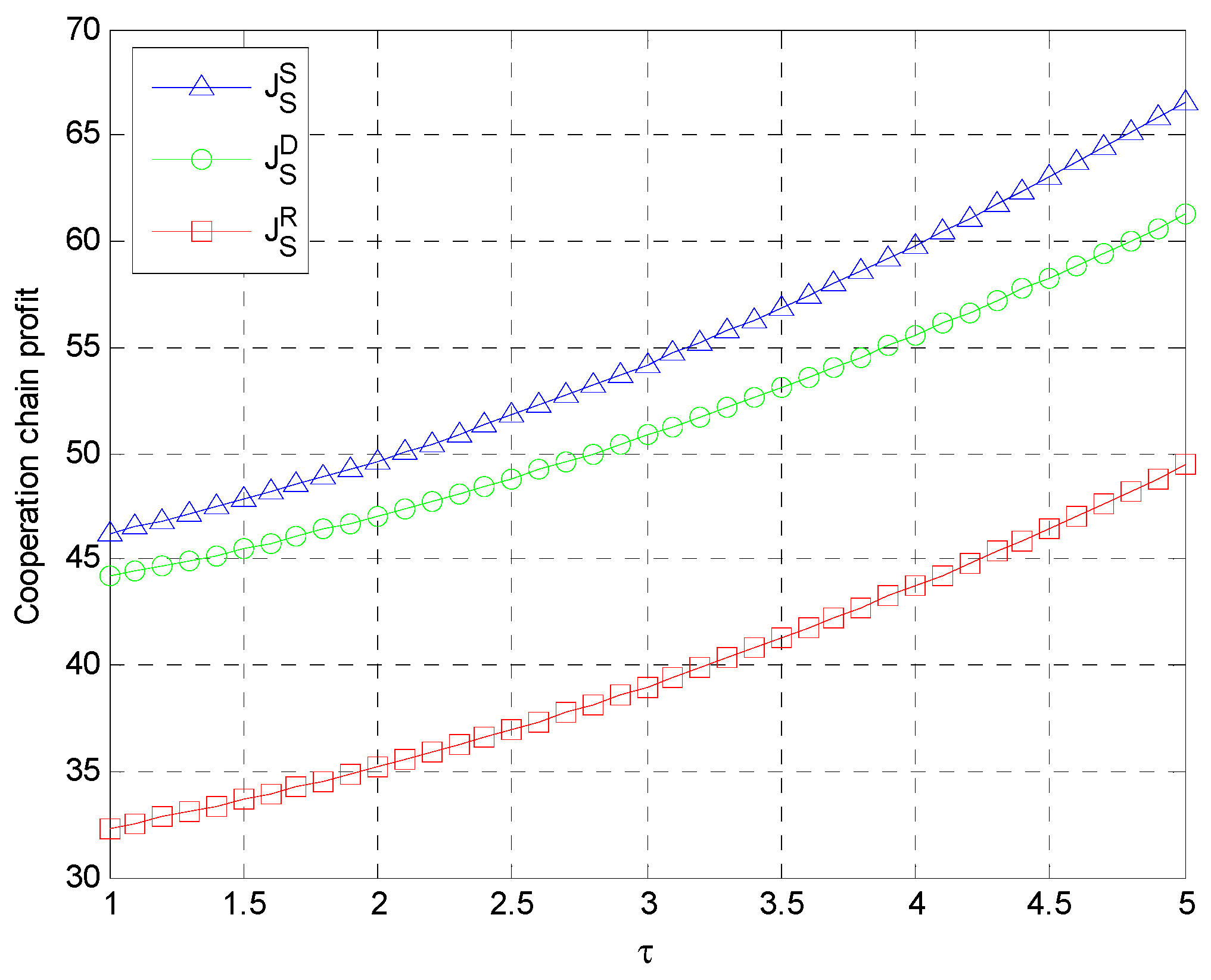
τ = (1.50→4.50)	+	+	×	×	+	+	+	+	+	+	+	+	+
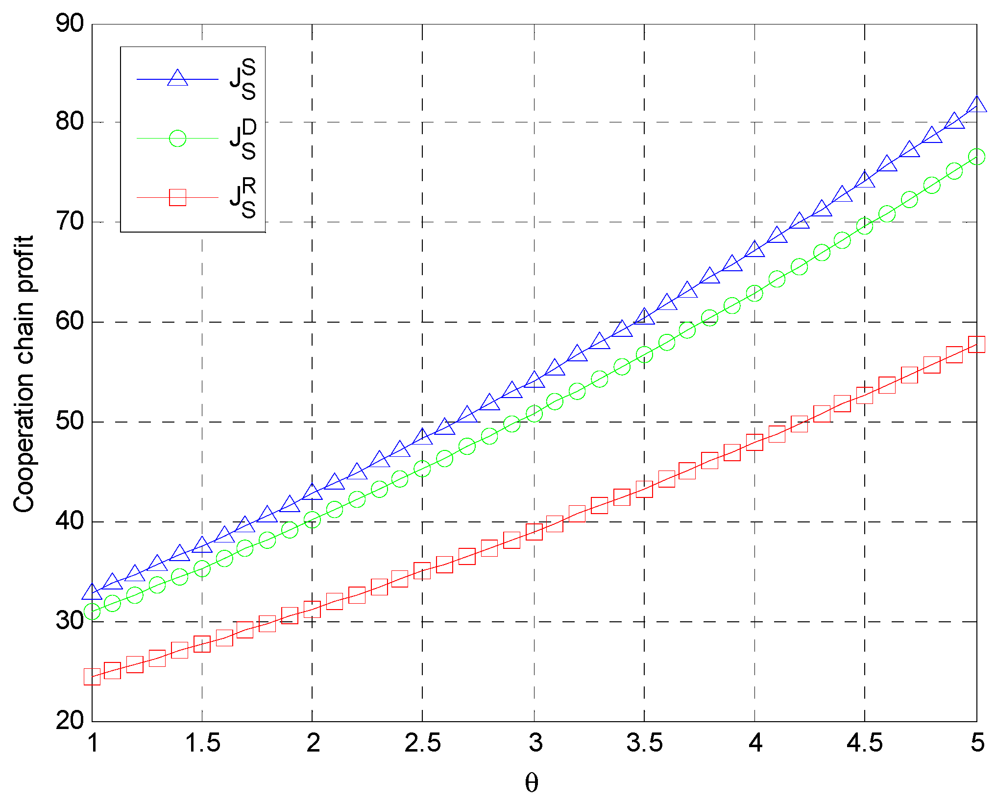
θ = (1.50→4.50)	+	+	+	+	+	+	+	+	+	+	+	+	+
ρ = (0.15→0.45)	−	−	−	−	−	−	−	−	−	−	−	−	−
μG = (0.50→1.50)	−	−	−	−	×	×	−	−	−	−	−	−	−
μM = (0.50→1.50)	×	×	×	×	−	−	−	−	−	−	−	−	−

ϖ = 0.4 under this set of parameters; “+” denotes increase; “−” denotes decrease; and “×”denotes invariability state.

and Figure 3, Figure 4, Figure 5 and Figure 6.

In the range of the model parameters given in the aforementioned example, it can be concluded that the same parameters, except ϖ, have the same influence on the trends with the same variables under three cases in Table 1. In this case, we further select some key parameters for further numerical simulation. Given the limited space available, this study only analyzes the pollution abatement cost coefficient of polluting enterprises (µ_M), the regional low-carbon natural decay rate (ϕ), the degree of pollution abatement efforts (τ), and the influence coefficient of the regional low-carbon degree (θ) to the optimal profit of the regional cooperation system. See the examples in Figure 3, Figure 4, Figure 5 and Figure 6, which describe the optimal profit function curves of the three decision-making modes under the above parameters. Other parameters, such as the local government contamination control cost coefficient (µ_G), local government contamination prevention efforts (δ), and the discount factor (ρ), have similar effects on the optimal profit function, so these shall not be covered again here.

As seen from Figure 3 and Figure 4, as the local government’s contamination control cost coefficient (µ_M) and the natural decay rate (ϕ) rise, the gradient of optimal profit in the regional low-carbon emission abatement system under three decision-making modes gradually declines at the same time point, indicating that the higher the investment of a pollution enterprise’s unit emission abatement (µ_M), the weaker the vertical regional low-carbon collaboration emission abatement effects; that is, the gradient of optimal profit in the regional low-carbon cooperation channel shall be smaller at the same time point. Similarly, together with the popularity of low-carbon concepts and the transformation of economic systems, the emission abatement effects of regional low-carbon vertical collaboration become much weaker as the regional low-carbon natural decay rate (ϕ) is expedited. Furthermore, the optimal profit to be gained by the entire cooperation chain under the coordinated joint carbon reduction model evidently surmounts that under the two decentralized schemes.

As seen from Figure 5 and Figure 6, along with the increase in emission abatement efforts of the polluting enterprise (τ) and the influence coefficient of regional low-carbon degree (θ), the gradient of optimal profits in the low-carbon cooperation chain under three decision-making modes gradually increases at the same time point, indicating that through adjusting production and business activities, the higher effect of the polluting enterprise in abating carbon emissions (τ), the better the vertical regional low-carbon collaboration emission abatement effects. That is, the gradient of optimal profits in the regional low-carbon emission abatement n system shall be greater at the same time point. Similarly, as the influence coefficient of the regional low-carbon degree (θ) turns more sensitive, the emission abatement effects are progressively evident in regional low-carbon vertical collaboration. In the meantime, compared with the two non-collaborative distributed contracts, the integrated channel gains more income.

7. Conclusions

In the low-carbon context, taking into consideration the influences of the emission abatement strategy on the regional low-carbon development level, this study introduces the time factor, and supposes the government contamination governance level and enterprise emission abatement ability as linear increasing functions of the regional low-carbon level. On that basis, three differential game models are constructed to expound the dynamic coordination strategy problems of regional low-carbon vertical emission abatement cooperation under given diverse decision-making situations. Furthermore, the sensitivity of relevant parameters is analyzed adopting a numerical simulation approach. Generally, through solving and analyzing the model, the following results emerge: (1) Under both non-cost-sharing and cost-sharing contracts, the efforts of the local government’s contamination control and the polluting enterprise’s emission abatement ability are positively correlated correlation with income distribution (ϖ), the influence coefficient of regional low-carbon degree (θ), low-carbon efforts (δ or τ), and the marginal contribution rate (α or β), whereas they are negatively correlated with the discount factor (ρ), decay rate (ϕ), and cost coefficient (µ_G or µ_M). (2) In the case of 2/3 < ϖ < 1, the local government’s contamination control efforts shall not be changed under a cost-sharing contract, and should offer a certain emission abatement cost subsidy to the enterprise, thus further mobilizing the enterprise to initiatively abate the emission. (3) Under the coordinated joint carbon reduction model, both the efforts of local government’s contamination control and the enterprise’s emission abatement are peaked, and the optimal trace of the regional low-carbon emission abatement system in the centralized case is also considerably larger relative to the non-collaborative decentralized mode. (4) In comparison with the non-collaborative emission abatement decisions, both the cooperation strategies of the local government and enterprise could encourage the two parties to invest more efforts in contamination control and emission abatement, and lead to them gaining more overall income in the regional carbon abatement cooperation chain. In the low-carbon situation, this also implies that the two parties in the cooperation chain system not only factor in the optimization profit, but also abide by the triple bottom principle of “economy–society–environment” [60], and reckon with their own social responsibilities and impacts exerted by long-term production on the environment, while making vertical cooperation emission abatement dynamic decisions. (5) In order to judge whether the model is practicable, Tianjin is selected as an example to elucidate how the model could be adopted to a realistic society. Besides the comparative analysis of regional low-carbon optimal traces in three different conditions with numerical examples, a sensitivity analysis is also performed on the impacts exerted by partial parameters on the optimal profit of the entire regional low-carbon emission abatement system. The shortcoming of this study is that it only observes the differential game relationship between a single local government and one enterprise subject. Yet, in practice, the strategic behavior between these two parties is a dynamic and complex relationship system. Future studies could factor in the low-carbon cooperation problems between government and firms in a multi-enterprise competition context, the contribution of different cooperation modes on regional emission abatement, and the impact of carbon tax, carbon transactions, and other policy constraints on regional low-carbon strategies.

References

- Meng, F.Y.; Su, B.; Thomson, E.; Zhou, D.Q.; Zhou, P. Measuring China’s regional energy and carbon emission efficiency with DEA models: A survey. Appl. Energy 2016, 183, 1–21. [Google Scholar] [CrossRef]
- Global Carbon Atlas. 2017. Available online: http://www.globalcarbonatlas.org/en/CO2-emissions (accessed on 25 January 2018).
- United Nations Framework Convention on Climate Change (UNFCCC). Intended National Determined Contributions (INDC) Submissions, 2015. Available online: http://www4.unfccc.int/Submissions/INDC/Submission%20Pages/submissions.aspx (accessed on 25 January 2018).
- Mi, Z.F.; Meng, J.; Guan, D.B.; Shan, Y.L.; Song, M.L.; Wei, Y.M.; Liu, Z.; Hubacek, K. Chinese CO2 emission flows have reversed since the global financial crisis. Nat. Commun. 2017, 8, 1712. [Google Scholar] [CrossRef] [PubMed]
- Mi, Z.F.; Meng, J.; Guan, D.B.; Shan, Y.L.; Liu, Z.; Wang, Y.T.; Feng, K.S.; Wei, Y.M. Pattern changes in determinants of Chinese emissions. Environ. Res. Lett. 2017, 12, 1–10. [Google Scholar] [CrossRef]
- Lin, B.Q.; Xin, Y.; Liu, X.Y. The strategic adjustment of China’s energy use structure in the context of energy-saving and carbon emission-reducing initiatives. Soc. Sci. China 2010, 1, 58–71. [Google Scholar]
- China Environmental State Bulletin. 2016. Available online: http://www.zhb.gov.cn/hjzl/zghjzkgb/lnzghjzkgb/201706/P020170605833655914077.pdf (accessed on 25 January 2018).
- Liu, H.; Zhang, Y.L.; Bi, J. Scenario analysis of China’s low-carbon development at local level-the case of Jiangsu Province, China. Popul. Resour. Environ. 2011, 4, 10–18. [Google Scholar]
- Zhao, L.M.; Chen, Z.J.; Liu, J.Y. Low-carbon cooperative strategy between government and enterprise based on differential games. Syst. Eng. 2016, 1, 84–90. [Google Scholar]
- Li, Z.; Zhang, M. A political economics analysis on China’s regional low-carbon competitiveness: Theory and empirical test. J. Financ. Econ. 2016, 42, 33–144. [Google Scholar]
- Tu, J.M.; Li, X.Y.; Guo, Z.C. Conception of enterprise carbon budget embedded in comprehensive budget system under low-carbon economy. China Ind. Econ. 2014, 3, 147–160. [Google Scholar]
- Montgomery, W.D. Markets in licenses and efficient pollution control programs. J. Econ. Theory 1972, 3, 395–418. [Google Scholar] [CrossRef]
- Zhang, L.M.; Yang, W.; Yuan, Y.; Zhou, R. An integrated carbon policy-based interactive strategy for carbon reduction and economic development in a construction material supply chain. Sustainability 2017, 9, 2107. [Google Scholar] [CrossRef]
- Zeng, S.H.; Nan, X.; Liu, C.; Chen, J.Y. The response of the Beijing carbon emissions allowance price (BJC) to macroeconomic and energy price indices. Energy Policy 2017, 106, 111–121. [Google Scholar] [CrossRef]
- Abildtrup, J.; Jensen, F.; Dubgaard, A. Does the Coase theorem hold in real markets? An application to the negotiations between waterworks and farmers in Denmark. J. Environ. Manag. 2012, 93, 169–176. [Google Scholar] [CrossRef] [PubMed]
- Chew, I.M.L.; Tan, R.R.; Foo, D.C.Y.; Chui, A.S.F. Game theory approach to the analysis of inter-plant water integration in an eco-industrial park. J. Clean. Prod. 2009, 17, 1611–1619. [Google Scholar] [CrossRef]
- Liao, Z.L.; Zhu, X.L.; Shi, J.R. Case study on initial allocation of Shanghai carbon emission trading based on Shapley value. J. Clean. Prod. 2015, 103, 338–344. [Google Scholar] [CrossRef]
- Yi, H.T.; Feiock, R.C.; Berry, F.S. Overcoming collective action barriers to energy sustainability: A longitudinal study of climate protection accord adoption by local governments. Renew. Sustain. Energy Rev. 2017, 79, 339–346. [Google Scholar] [CrossRef]
- Zhang, Z.G.; Jin, X.C.; Yang, Q.X.; Zhang, Y. An empirical study on the institutional factors of energy conservation and emissions reduction: Evidence from listed companies in China. Energy Policy 2013, 57, 36–42. [Google Scholar] [CrossRef]
- Zeng, S.H.; Liu, Y.C.; Liu, C.; Nan, X. A review of renewable energy investment in the BRICS countries: history, models, problems and solutions. Renew. Sustain. Energy Rev. 2017, 74, 860–872. [Google Scholar] [CrossRef]
- Wu, J.; Chang, I.S.; Yilihamu, Q.; Zhou, Y. Study on the practice of public participation in environmental impact assessment by environmental non-governmental organizations in China. Renew. Sustain. Energy Rev. 2017, 74, 186–200. [Google Scholar] [CrossRef]
- Li, Q.W.; Long, R.Y.; Chen, H. Empirical study of the willingness of consumers to purchase low-carbon products by considering carbon labels: A case study. J. Clean. Prod. 2017, 161, 1237–1250. [Google Scholar] [CrossRef]
- Wirl, F. Social interactions within a dynamic competitive economy. J. Optim. Theory Appl. 2007, 133, 385–400. [Google Scholar] [CrossRef]
- Song, B.D.; Ko, Y.D. Effect of inspection policies and residual value of collected used products: A mathematical model and genetic algorithm for a closed-loop green manufacturing system. Sustainability 2017, 9, 1589. [Google Scholar] [CrossRef]
- Su, B.; Thomson, E. China’s carbon emissions embodied in (normal and processing) exports and their driving forces, 2006–2012. Energy Econ. 2016, 59, 414–422. [Google Scholar] [CrossRef]
- Yin, J.H.; Zheng, M.Z.; Chen, J. The effects of environmental regulation and technical progress on CO2 Kuznets curve: An evidence from China. Energy Policy 2015, 77, 97–108. [Google Scholar] [CrossRef]
- Su, B.; Ang, B.W. Multiplicative structural decomposition analysis of aggregate embodied energy and emission intensities. Energy Econ. 2017, 65, 137–147. [Google Scholar] [CrossRef]
- Xia, X.H.; Hu, Y.; Chen, G.Q.; Alsaedi, A.; Hayat, T.; Wu, X.D. Vertical specialization, global trade and energy consumption for an urban economy: A value added export perspective for Beijing. Ecol. Model. 2015, 318, 49–58. [Google Scholar] [CrossRef]
- Li, C.S.; Fan, Y.; Zhu, L. The study of carbon dioxide emission intensity abatement mechanism of iron and steel industry based on two-stage game model. Chin. J. Manag. Sci. 2012, 2, 93–101. [Google Scholar] [CrossRef]
- Li, Y.; Zhao, D.Z.; Zhu, X.G. A game model for government and enterprise behavior based on a carbon tax. Resour. Sci. 2013, 1, 125–131. [Google Scholar]
- Decanio, S.J.; Fremstad, A. Game theory and climate diplomacy. Ecol. Econ. 2013, 85, 177–187. [Google Scholar] [CrossRef]
- Zhang, G.X.; Zhang, X.T.; Cheng, S.J.; Chai, G.R.; Wang, L.L. Signaling game model of government and enterprise based on the subsidy policy for energy saving and emission reduction. Chin. J. Manag. Sci. 2013, 21, 129–136. [Google Scholar]
- Zhao, R.; Zhou, X.; Han, J.J.; Liu, C.L. For the sustainable performance of the carbon reduction labeling policies under an evolutionary game simulation. Technol. Forecast. Soc. Chang. 2016, 112, 262–274. [Google Scholar] [CrossRef]
- Jørgensen, S.; Zaccour, G. Time consistent side payments in a dynamic game of downstream pollution. J. Econ. Dyn. Control. 2001, 25, 1973–1987. [Google Scholar] [CrossRef]
- Huang, Z.S.; Nie, J.J.; Tsai, S.B. Dynamic collection strategy and coordination of a remanufacturing closed-loop supply chain under uncertainty. Sustainability 2016, 9, 683. [Google Scholar] [CrossRef]
- Yeung, D.W.K.; Petrosyan, L.A. Subgame consistent solutions of a cooperative stochastic differential game with nontransferable payoffs. J. Optim. Theory Appl. 2005, 124, 701–724. [Google Scholar] [CrossRef]
- Guo, D.X.; Wu, Y.Y.; Xu, Q.Y. Analysis of supply chain under different subsidy policies of the government. Susainability 2016, 8, 1290. [Google Scholar] [CrossRef]
- Jørgensen, S.; Zaccour, G. A survey of game-theoretic models of cooperative advertising. Eur. J. Oper. Res. 2014, 237, 1–14. [Google Scholar] [CrossRef]
- Yeung, D.W.K.; Petrosyan, L.A. Subgame consistent cooperative solution for NTU dynamic games via variable weights. Automatica 2015, 59, 84–89. [Google Scholar] [CrossRef]
- Benchekroun, H.; Martín-Herrán, G. The impact of foresight in a tansboundary pollution game. Eur. J. Oper. Res. 2016, 251, 300–309. [Google Scholar] [CrossRef]
- Bertinelli, L.; Camacho, C.; Zou, B.T. Carbon capture and storage and transboundary pollution: A differential game approach. Eur. J. Oper. Res. 2014, 237, 721–728. [Google Scholar] [CrossRef]
- Wang, Z.H.; Yang, L. Delinking indicators on regional industry development and carbon emissions: Beijing-Tianjin-Hebei economic band case. Ecol. Indic. 2015, 45, 41–48. [Google Scholar] [CrossRef]
- Jørgensen, S.; Taboubi, S.; Zaccour, G. Retail promotions with negative brand image effects: Is cooperation possible? Eur. J. Oper. Res. 2003, 150, 395–405. [Google Scholar] [CrossRef]
- Breton, M.; Sokri, A.; Zaccour, G. Incentive equilibrium in an overlapping-generations environmental game. Eur. J. Oper. Res. 2008, 185, 687–699. [Google Scholar] [CrossRef]
- Chen, Q.X.; Kang, C.Q.; Ming, H.; Wang, Z.Y.; Xia, Q.; Xu, G.X. Assessing the low-carbon effects of inter-regional energy delivery in China’s electricity sector. Renew. Sustain. Energy Rev. 2014, 32, 671–683. [Google Scholar] [CrossRef]
- Zaccour, G. On the coordination of dynamic marketing channels and two-part tariffs. Automatica 2008, 44, 1233–1239. [Google Scholar] [CrossRef]
- Dockner, E.J.; Van Long, N. International pollution control: Cooperative versus noncooperative strategies. J. Environ. Econ. Manag. 1993, 25, 13–29. [Google Scholar] [CrossRef]
- Yu, W.; Han, R.Z. Coordinating a two-echelon supply chain under carbon tax. Sustainability 2017, 12, 2360. [Google Scholar] [CrossRef]
- Qin, F.F.; Zhang, X.N. Designing an optimal subsidy scheme to reduce emissions for a competitive urban transport market. Sustainability 2015, 7, 11933–11948. [Google Scholar] [CrossRef]
- Wei, C.; Ni, J.L.; Du, L.M. Regional allocation of carbon dioxide abatement in China. China Econ. Rev. 2012, 23, 552–565. [Google Scholar] [CrossRef]
- Chen, J.X.; Chen, J. Supply chain carbon footprinting and responsibility allocation under emission regulations. J. Environ. Manag. 2017, 188, 255–267. [Google Scholar] [CrossRef] [PubMed]
- Yang, L.; Zhang, Q.; Ji, J. Pricing and carbon emission reduction decisions in supply chains with vertical and horizontal cooperation. Int. J. Prod. Econ. 2017, 191, 286–297. [Google Scholar] [CrossRef]
- Eyland, T.; Zaccour, G. Carbon tariffs and cooperative outcomes. Energy Policy 2014, 65, 718–728. [Google Scholar] [CrossRef]
- Wei, Y.M.; Mi, Z.F.; H, Z.M. Climate policy modeling: An online SCI-E and SSCI based literature review. Omega 2015, 57, 70–84. [Google Scholar] [CrossRef]
- Air Pollution Prevention and Control Action Plan. 2013. Available online: http://www.gov.cn/zhengce/content/2013-09/13/content_4561.htm (accessed on 27 January 2018).
- Beijing-Tianjin-Hebei Reinforcement Measures for Air Pollution Control (2016–2017). 2016. Available online: http://www.envsc.net/file/201609301225182778.pdf (accessed on 27 January 2018).
- Law of the People’s Republic of China on Prevention and Control of Atmospheric Pollution. 2016. Available online: http://www.zhb.gov.cn/gzfw_13107/zcfg/fl/201605/t20160522_343394.shtml (accessed on 27 January 2018).
- Tianjin Environmental Statement. 2016. Available online: http://www.tjhb.gov.cn/root16/mechanism/standard_monitoring_of_the_Department_of_science_andtechnology/201706/P020170605593040876560.pdf (accessed on 27 January 2018).
- Ambient Air Quality Standards. 2012. Available online: http://kjs.mep.gov.cn/hjbhbz/bzwb/dqhjbh/dqhjzlbz/201203/W020120410330232398521.pdf (accessed on 28 January 2018).
- Jørgensen, S.; Martín-Herrán, G.; Zaccour, G. Dynamic games in the economics and management of pollution. Environ. Model. Assess. 2010, 15, 433–467. [Google Scholar] [CrossRef]