A Sustainable Industry-Environment Model for the Identification of Urban Environmental Risk to Confront Air Pollution in Beijing, China

1
School of Law, Capital University of Economics and Business, Beijing 100072, China
2
School of Labor Economics, Capital University of Economics and Business, Beijing 100072, China
3
Department of Building, Civil and Environment Engineering, Concordia University, Montreal, QC H3G 1M8, Canada
4
MOE Key Laboratory of Regional Energy Systems Optimization, Sino-Canada Energy and Environmental Research Center, North China Electirc Power University, Beijing 102206, China, [email protected]
*
Author to whom correspondence should be addressed.
Sustainability 2018, 10(4), 962; https://doi.org/10.3390/su10040962
Submission received: 13 March 2018
/
Revised: 20 March 2018
/
Accepted: 22 March 2018
/
Published: 26 March 2018
Abstract
:In this study, an optimized industry-environment model is proposed for identifying environmental risk under uncertainties. The strategy associated with an emission-permit trading mechanism has been introduced into the industrial-environment regulation (model) for remitting the pressures of frequent/severe haze events in Beijing City. A dual stochastic mixed fuzzy risk analysis method with Laplace’s criterion (DSFRL) can be embedded into industry-environment issues with a trading emission-permit trading mechanism (IEST) for handling uncertainties regarded as possibility and probability distributions. Meanwhile, this can also reflect the environmental risks and corresponding system benefits due to the occurrence of a random event (such as random wind velocity). Based on the application of the proposed IEST with DSFRL, the numbers of the obtained results associated with production reduction, adjustment of industrial layout pattern, emission-permit transactions, pollutant mitigation and system benefits under various Laplace criterion cases can be analyzed. A tradeoff between production development and pollution mitigation based on the preference of policymakers can be used for rectifying current strategies with a sustainable mode, which can prompt an effort to confront air pollution
1. Introduction
Against the background of rapid urbanization/industrialization, high-speed economic development has greatly improved human lives across the world, but has also brought about detrimental pressures on the air environment. Particularly in a number of fast-growing cities such as Beijing, China, the accelerated exploitation of industry and disorderly industrial layouts can generate excessive pollutant emissions, which exceed what the environmental load can afford, generating environmental risks. From 2013, environmental risks associated with haze events of atmospheric pollution have been frequent. Given the hazed concentration of fine particulate matter (e.g., PM2.5) and traditional pollutants (including SO2, NO2, and PM10), the incidence of respiratory system diseases due to air pollution has presented an increasing trend. Meanwhile, other damage to cardiovascular/cerebrovascular systems and nervous systems in terms of public health have been reported frequently in response to air pollution. Thus, the air pollution issue can give rise to a health risk in Beijing, which is today challenging policymakers [1,2,3]. Against the stresses of air pollution, a number of anthropogenic engineering techniques (including engineering control measures, clean production techniques, environmental regulation policy and an industrial adjustment strategy) have been advocated to confront such hazardous air pollution issues. Among them, pollutant emission-permit trading is an effective method which can facilitate pollutant permits from a lower to higher value in order to achieve gains in economic efficiency, but also can provide incentives to adopt pollution abatement measures [4]. Meanwhile, a market approach can drive industrial companies to improve the efficiency of pollutant treatments, with the aim of avoiding a higher environmental penalty or cost for buying the emission permit. Moreover, a trading mechanism-based (TM) can adjust the scale and structure of emissions to improve the efficiency of production at the extreme, leading to greater system benefit. Therefore, an optimized industry-environment strategy with an emission-permit trading mechanism (IEST) is desirable for coordinating the relationship between the development of the economy and the protection of the environment in Beijing, reducing the environmental risk and damage to public health [5,6].
However, an IEST issue is complicated with a number of objective and subjective uncertainties, leading to complexities. Above all, uncertainties and their corresponding complexities can increase the risk for policymakers to generate the desired decision alternatives [7]. Previously, many research works such as genetic algorithms, potential economic impact assessments, the asymmetric fuzzy method and the inexact stochastic programming model have been developed for handling inherent uncertainties in the decision process of an IEST issue, which can reduce the difficulties and risk levels of decision-making [8,9,10,11,12,13]. Among them, two-stage stochastic programming (TSP) is a useful method to deal with random problems through rectifying actions (i.e., recourse action with probabilistic event). For example, meteorological conditions in an IEST issue can influence the diffusion and migration processes of pollutants, which can result in random concentration levels. If these levels exceed standards regulated by a government, this implies the random events of air pollution may occur at several times or last a few days. These random hazed air pollution incidents can bring about environmental loss to the first-stage decisions (e.g., economic development targets) periodically over time through TSP [14]. However, this cannot reflect the variability of the second-stage decisions, where a high-variability level of risk violation would challenge policymakers [15]. Therefore, a risk control analysis method (RAM) is proposed to capture variable risk in a TSP contest, which can control the variability of the recourse values (e.g., pollutant penalty) in a rational range [16]. Nevertheless, in an IEST issue, the economic and environmental strategy with scenario assumptions can be also expressed as probabilistic distributions, which result in dual stochastic situations. A stochastic Laplace criterion (SLC) is introduced to handle the probability of each scenario occurrence under the supposition of no data being available on the probabilities of the various outcomes [17,18]. Meanwhile, a number of fuzzy occurrences in an IEST issue (such as missing economic data, an imprecise diffusion process and fuzzy trading efficiency) can intensify the risk of the decision-making process. For example, in an IEST issue, the diffusion or migration process of pollution is regarded as fuzziness since it is often difficult to calculate accurately. Therefore, a fuzzy credibility constraint programming (FCP) can be included while handling of this precise information in goals or constraints with a high satisfaction degree [19,20]. Previously, few works have focused on multiple uncertainties in hybrid formats in an IEST planning issue.
Thus, the objective of this study is to propose an optimized industry-environment strategy with an emission-permit trading mechanism (IEST) for alleviating production-emission conflict in Beijing. A dual stochastic mixed fuzzy risk analysis method with Laplace’s criterion (DSFRL) can be embedded into an IEST issue, which can deal with fuzzy and dual stochastic uncertainties in a two-stage context. Meanwhile, it can also reflect and control the risk of a two-stage decision in a rational range according to risk exposure and aspiration benefit levels. The application in Beijing has shown that market trading is an effective mechanism to confront severely diminished environmental capacity and aggravating air pollutant emissions. Results of emission-permit transactions, production reductions, pollution-abatement schemes, adjustment of industrial structures and system benefits under various cases are obtained and analyzed. The results show that a trading mechanism is a more effective method to adjust industrial layout and reduce air pollutant emission in the study region, as well as manage the air-environment crisis. Meanwhile, the risk-averse attitude and robustness coefficient can improve the reliability of decision-making in an IEST issue. These findings can support policymakers in identifying optimized industry-environment policies for coordinating the relationship between economic development and environmental protection, as well as controlling the air pollution crisis at an urban level.
2. Methodology
2.1. Two-Stage Stochastic Programming for Risk Control (TSR)
In a decision-making problem, two-stage stochastic programming (TSP) can built a linkage between expected targets and a random event, where the first-stage benefit can be rectified by a second penalty as follows [21]:
In Model 1, a recourse action occurs between (i.e., first-stage benefit) and (i.e., second-stage penalty), where is random event after the first-stage decision has been made; and the denotes as the probability of realization of event . However, TSP can not control the risk of recourse action against any infeasibilities under various scenarios (h). If an excessive penalty exceeds what the system can afford, it can bring about systemic failure. Therefore, a risk-control method can be joined into a two-stage context [16]:
where if the actual benefit (i.e., ) is smaller than the expected target, the probability (i.e., ) that presents the targeted benefit cannot be met under various scenarios h would be 1, otherwise, it would be 0 [18]. Thus, a risk control based TSP can be expressed as follows:
where is a binary variable defined for each scenario; is the allowable risk exposure level; is target level; is the balancing benefits for scenario h and target level (). In fact, the probability of not meeting the targeted benefit in each scenario would be either 0 or 1.
2.2. Dual Stochastic Programming for Risk Control with Laplace’s Criterion Scenario Analysis (DSLS)
However, in a practical IEST issue, the input of the expected target (i.e., the first-stage decision variable) can be influenced by various factors, which would be tackled by a scenario analysis (SA) [20]. In general, the risk attitudes of policymakers can impact the generation of a scenario due to their experiences and personality traits. Thus, the definition of a stochastic scenario analysis (SSA) can be expressed as follows:
where is the decision outcome; is payoff matrix row, (); is probability of each scenario occurrence; d is the option; D is the options; is the overall performance; is the progressive scenario, which means that progressive target with optimism attitude; is the conservative scenario, which means that conservative target with pessimism attitude; m2 is the numbers of scenarios; among them, m1 is the number of progressive scenarios; (m2 − m1) is the number of conservative scenarios. However, since the scenario of each scenario is random, this results in policymakers having difficulty in decision making. Laplace’s criterion can handle the probability of each scenario occurrence under the supposition of no data available on the probabilities of the various outcomes, which can be formulated as follows [17,18]:
Based on TSR, dual stochastic programming for risk control with Laplace’s criterion scenario analysis (DSLS) can be modified as follows:
Subject to:
2.3. A Dual Stochastic Mixed Fuzzy Risk Analysis Method with Laplace’s Criterion (DSFRL)
Nevertheless, a number of uncertainties related to precise estimation and fuzziness cannot handle probabilistic distributions [21]. Therefore, fuzzy credibility constrained programming (FCP) can be advocated as follows:
Based on the concept of fuzzy credibility, the credibility measure (Cr) can be expressed as [22]. In general, the credibility level should be greater than 0.5 usually [23]. Thus, the model (6a) can be proven as follows:
Thus, a dual stochastic mixed fuzzy risk control method (DFR) can be resolved as follows:
Subject to:
3. Application
3.1. Overview of the Study Area
Beijing is located on the North China Plain, which covers an area of 16,807.8 km2. The city has 18 districts, with a population of more than 21.71 × 10⁶ people (at the end of 2015). As the capital of China, it has grown fast in recent years. In 2015, the GDP reached 2296.8 billion Yuan, and it has maintained a high growth rate of about 6.90% in recent years. Meanwhile, the growth rate of the population has been maintained at 9.00‰ per year [24,25]. In the context of rapid urbanization/industrialization, industry has developed rapidly. The establishment of a modern agricultural structure, developing a peri-city modernistic industry, and prioritizing tourism have promoted living standards and social material productivity [24]. Due to the expansion of industry, large-scale pollutant discharges have exceeded what the natural environment can afford, which results in frequent haze events of air pollution.
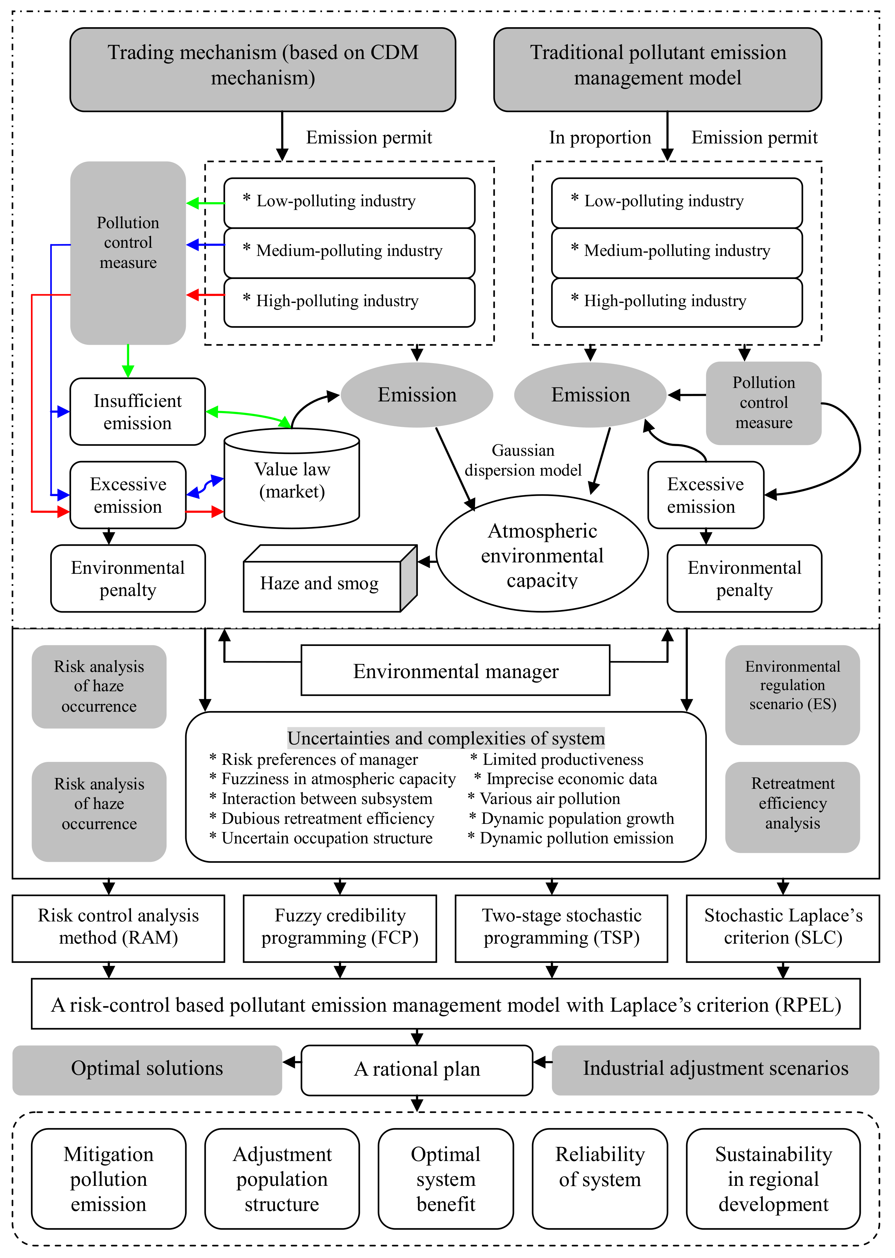
Figure 1 displays the framework of a risk-control based pollutant emission management model with Laplace’s criterion (RPEL) and its application in the study region. In order to confront the air pollution issue, policymakers have built a linkage between “production” and “emission” for the adjustment of production, which can reduce pollutant emissions. In a traditional urban industry-environment model, enterprises would reduce the scale of production to confront the environmental penalty. However, a single political plan cannot conserve the environment at the extremes due to “governance failure”. Thus, a market approach is joined with industrial-environment regulation to reallocate emission permits from lower to higher values. This can increase economic efficiency overall, meanwhile providing incentives to adopt pollution abatement. In an optimized industry-environment strategy with an emission-permit trading mechanism (IEST) issue, the regional policymakers must create a plan to allocate emission permits to every enterprise and maximize the overall system benefit. Based on an initial emission obligation, the enterprise can buy or sell the emission permit in the market, remedying their emission deficit or releasing their excessive permits. Otherwise, excessively polluting enterprises have to pay the higher environmental penalty due to their emission-permit deficit. The trading mechanism can facilitate enterprise to improve the efficiency of pollutant retreatment and productivity, which can be beneficial for confronting the higher environmental penalty. The tradeoff between economic development and emission abatement can generate a comprehensive plan associated with pollution control. However, in an IEST issue, there are a variety of factors such as on-site surveying and monitoring, the analysis of the main affected factors, the determination of pollution-source emission standards, the partition of functional zones, and the design of their respective environmental capacities, as well as the generation of control measures [26]. Thus, a dual stochastic mixed fuzzy risk analysis method with Laplace’s criterion (DSFRL) is proposed to handle these objective and subjective uncertainties in an IEST system. Therefore, the steps of the RPEL method applied in an IEST issue in the study region can be formulated as follows:
- Step 1:
- Recognition of the regional features of economic development, production scale, pollutant emission and meteorological conditions in Beijing.
- Step 2:
- Construction of a linkage of production-emission to reflect the relationship between production scale/structure and pollutant emission in the study region.
- Step 3:
- Establishment of an emission-permit trading mechanism to reallocate the emission permit from lower to higher value, regulating the regional production layout and emission scale.
- Step 4:
- Identification of various uncertainties and their interactions in an IEST issue in Beijing.
- Step 5:
- Incorporation of two-stage stochastic programming, risk-analysis control method, Laplace scenario and fuzzy credibility programming into a framework to propose a RPEL method to deal with multiple uncertainties in an IEST issue.
- Step 6:
- Formulation of a sustainable industry-environment model for identifying environmental risk under uncertainties and meanwhile calculating optimized results. The model has been calculated by Lingo 12.0, that has the advantage of providing a capacity to deal with unlimited variables and constraints in a friendly way compared to ORS, WinQSB and Matlab. The Lingo 12.0 is an effective tool for policymakers to describe the complex system and interactions among components based on a series of equations and functions.
- Step 7:
- Analysis of obtained results associated with production reduction, adjustment of industrial layout patterns, emission-permit transactions, pollutant mitigation and system benefits under various Laplace criterion cases.
- Step 8:
- Generation of a sustainable industry-environment plan to adjust regional strategies to conform integrity between the regional economy and environment. Complete a plan process.
3.2. Modeling Formulation
Based on the DSFRL method, an optimized industry-environment strategy with emission-permit trading mechanism (IEST) is formulated. The policymakers should consider the issues as follows: (a) how to balance the relationship between economy and environment to confront urban diseases and the air crisis; (b) how to introduce a trading mechanism to improve the production mode and efficiency of pollutant mitigation; (c) how to adjust the current industrial production scale and pollutant emission permit based on a trading mechanism to meet air-quality standards in the study region; (d) how to generate a reliable plan against environmental risk. Thus, an optimized industry-environment with emission-permit trading mechanism (IEST) through DSFRL method can be formulated as follows:
(1) Benefits from various industrial sectors based on expected economic development (IIP):
(2) Environmental penalty for excessive emission from industrial sectors (PEP):
(3) Loss for reduced production according to adjustment of industrial structure (LRP):
(4) Environmental retreatment cost of various industrial sectors (CER):
(5) System benefit from emission-permit transaction (BET):
(6) Cost for emission-permit transaction (CET):
The detailed nomenclatures for the variables and parameters is provided in the notation and subscript. Where is the green gross domestic product (GGDP) in Beijing, which equals the total system benefit of economy-added return from emission-permit trading minus the loss from reduced production, the environmental penalty for excessive emissions, retreatment costs and trading costs. In this study, industry is deemed to be the main source of pollutant emissions, which can be divided into three sources whereby high, medium and low pollution industries can be considered in the modelling formulation. Meanwhile, industrial productiveness, pollutant generation and retreatment efficiency can be included in the model to reflect various pollution patterns. Under these situations, varied constraints such as mitigation requirements, capacity of pollutant-mitigation, emission allowance, air quality, industrial structure and scale and non-negativity can be displayed as follows:
- (1)
- Pollutant-mitigation requirement:
- (2)
- Pollutant-mitigation capacity:
- (3)
- Available emission permit for transaction:
- (4)
- Ambient air-quality requirement:
- (5)
- Industrial production scale:
- (6)
- Economic risk based on DSFRL method:
- (7)
- Non-negativity:
Constraint (1) displays the demand of pollutant-mitigation in an IEST issue, where the pollutant emission from the industrial sector should be restricted by the regional environmental load. Constraint (2) shows the capacity of pollution mitigation according to current clean production techniques, where the discharged pollution can be processed with meteorological data (e.g., wind velocity). Constraint (3) presents the emission-permit transaction, which equals the expected pollutant emission minus maximum emission-permit allowance. This means that after the emission-permit is allocated to enterprises, if they discharge more pollutants that exceed their initial permit obligations they have to buy a permit from the market; otherwise, they have to afford the environmental penalty. Constraint (4) displays the ambient air quality based on the Gaussian dispersion model (GDM), where the wind velocity (i.e., ) expressed as fuzziness can be handled by credible measures (as shown in the “Methodology” section). Constraint (5) shows the scale of industrial development, which can be restricted by the minimum/maximum development scale in the study region. Constraint (6) presents economic risk based on the DSFRL method, which can reflect the risk between the expected benefit and the targeted value (as shown in the “Method” section). Constraint (7) is non-negativity restrictions.
3.3. Data Collection
A number of input parameters are calculated by government reports, statistical yearbooks, and related research work [24]. Table 1 displays economic data, where the net benefit of unit production and corresponding environmental penalty of excessive pollutant emission have been listed. They can be estimated according to the statistical yearbook of Beijing from 2000 to 2013, with consideration of the development of the economy [24,25].
Meanwhile, since the meteorological conditions (e.g., wind velocity) can influence the capacity of pollution diffusion, varied meteorological data (i.e., wind velocity) are provided in Table 2. The data can be obtained from the weather stations of Beijing. Through simulation and calculation, the levels of wind velocity and corresponding probabilities have been listed in Table 2. In the study region, the meteorological condition can impact the capacity of the diffusion of pollutant, which can be calculated by the Gaussian dispersion model (GDM) (as shown in “Modelling Formulation”). The coefficient of the Gaussian dispersion model can be estimated according to the Pasquill–Gifford curve [26].
In this study, the regulation of the concentrations of pollutant emission from the industrial section can be obtained from the ambient air-quality standard (GB 3095 2012) [27] in China, which can be denoted “AAQS”. Since Beijing confronts great air pollution stress, the air-quality requirement can be advanced to regional policymakers. From 2013, the Grade-II standard of the ambient air quality had been regulated, where the average maximum concentration limits of SO2, NO2, PM10 and PM2.5 were 60, 40, 70 and 35 μg/m3 per year, respectively. Based on these regulations of AAQS in Beijing, we have obtained the right-hand side of the constraint (4), where the future air-quality requirement can be calculated in the fuzzy credibility manner: (i.e., , , and ). Based on the Gaussian dispersion model (GDM), the concentration of pollutant from industrial sector emissions can be regulated by the maximum concentration limits of SO2, NO2, PM10 and PM2.5, the solution for the optimized industry-environment strategy with the emission-permit trading mechanism (IEST) can be calculated. The amount of air-pollutant emissions is calculated by production scales of various industrial sectors multiplied by their coefficients of pollutant emission, where the coefficients of pollutant emission are estimated from regional standards such as the Integrated Emission Standards of Air Pollutants (DB11/501 2017) [28].
Table 3 presents various cases associated with different risk attitudes of policymakers for developing the economy and protecting the environment, where 10 scenarios are designed to reflect different risk attitudes (Laplace scenarios).
4. Results
4.1. Emission Quality without Trading Mechanism
Figure 2 shows total excessive pollutant emissions under various cases when ε and α levels are 0.95 and 0.99, respectively. In this study, excessive pollutant emissions can bring about an increment of concentration of pollution in the air, which would influence public health. The results indicate that lower wind velocities would generate higher concentrations of pollution. For example, when wind velocity is at a high level, the ultra-concentration ratios of PM10 and PM2.5 were 3.23 and 0.52 times than when wind velocity is at a low level under case 1 in period 1. Meanwhile, the results show the highest ultra-concentration ratio of SO2 and NO2 would be 7.34 and 6.23 times compared to normal conditions due to bad meteorological conditions for diffusion. This demonstrate that the current industrial production mode (including scale of production, emission pattern and retreatment) is backward and cannot accommodate regional environmental regulation. Thus, adjustment of the pollution mitigation scheme, industrial structure and clean production technique should be required.
4.2. Analysis of Emission-Permit Trading Mechanism
4.2.1. Amount of Pollutant Emission-Permit Transaction
Figure 3 shows the transaction of the emission permit among various industrial sectors under case 1 when the ε and α levels are 0.95 and 0.99, respectively. From the results, several indications can be obtained as follows: (a) the buyer can buy an emission permit from the seller due its excessive emissions, especially when wind velocity is low. For example, when the wind velocity level is low, the total emission-permit transaction of NO2, SO2, PM10 and PM2.5 for a buyer (industry user) in IP would be 0.95, 3.75, 0.98 and 0.43 × 10³ ton under case 1. (b) Similarly, the buyer would release an emission permit to be traded through the market, where the emission-permit transaction would vary with different diffusion levels, and vice-versa. (c) In comparison with the total trading amounts of various industrial sectors, the greatest buyers of NO2, SO2, PM10 and PM2.5 are cement manufacturing (CM), iron processing (IP), CM and power generation (PG); and the greatest sellers are PM, chemical industry (CI), paper-msimilarg industry (PM) and chemical industry (CI).
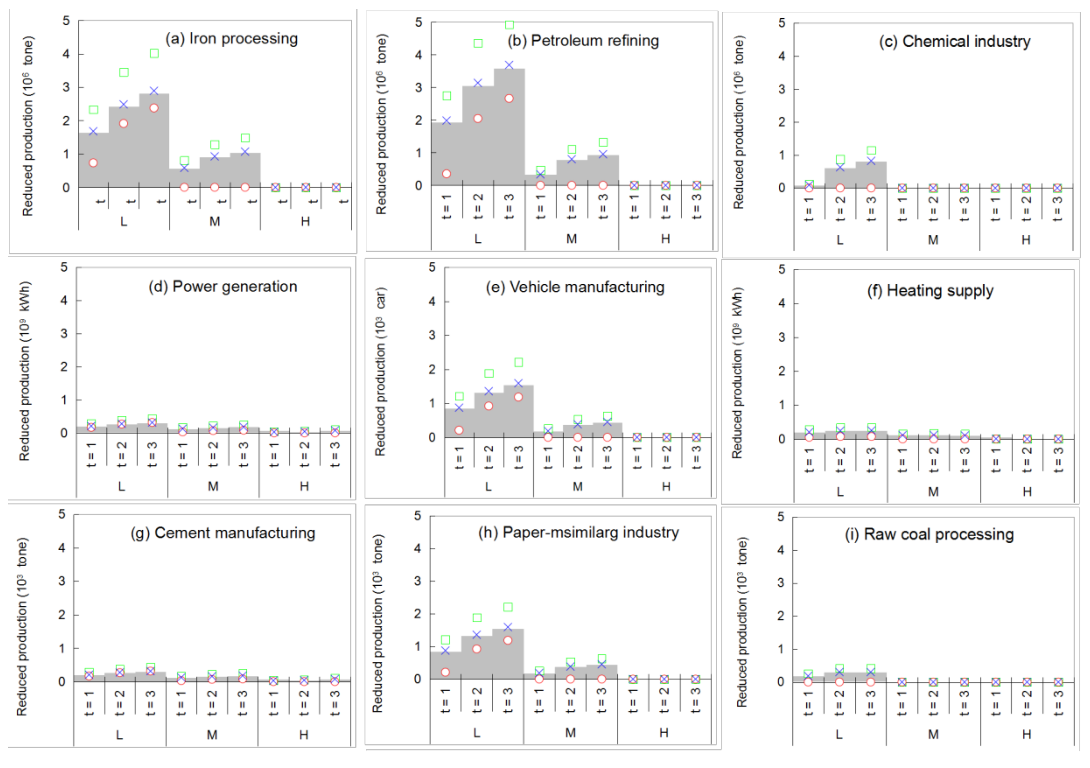
4.2.2. Production Scale Adjustment with Trading Mechanism
Figure 4 displays optimized reduced production among various industrial sectors under cases 1, 4, 8 and 10 when ε and α levels are 0.95 and 0.99, respectively. Based on the emission-permit transaction, a number of industrial companies should consider the penalties of excessive emissions to reduce the scale of production; otherwise, they have to buy emission permits. Through the calculation of the pollutant emission-permit transaction in Figure 2, a number of companies have obtained permits. However, their pollutant emissions have exceeded the allowance. Therefore, they have to reduce the scale of production. The results obtained from Figure 3 presenting the scales of reduced production would vary with different pollutant diffusion capacity such as wind velocity. In Beijing, higher wind velocity occurs in summer and autumn, which would be suitable for pollutant diffusion. Under these situations, the scales of reduced production would be relatively lower due to its higher capacity of diffusion, and vice-versa. Meanwhile, various production scales in different industrial sectors can generate varied reductions. In comparison, the industrial sector with the feature of higher pollutant emission and lower economic returns would be restricted first. For instance, iron processing (denoted as “IP”) with features of higher pollutant emission and lower economic returns can generate the highest reduction. This implies that current scale of IP and corresponding production mode would bring about and exorbitant environmental penalty, leading to reduced benefits. Thus, adjustment of the IP scale or the improvement of its production and emission modes would be required. Similar situations occurred in petroleum refining (denoted as “PR”) and power generation (denoted as “PG”) in response to their higher production scale, pollutant emissions and lower economic benefits. For instance, when wind velocity is at a low level in period 1, the reduced scale of production in PR, PG and IP would be 445.2 × 10⁶ tons, 244.3 × 10⁹ kwh and 594.4 × 10⁶ tons under case 1 (α = 0.95). By contrast, the reduced scale of vehicle manufacturing (denoted as “VM”) and chemical industry (denoted as “CI”) are relatively lower than in PG, PR and IP due to their lower scales of pollutant emission. This implies that their scales of production are relatively rational, since their scales of production were within the limits of environmental capacity.
4.3. Risk Analysis
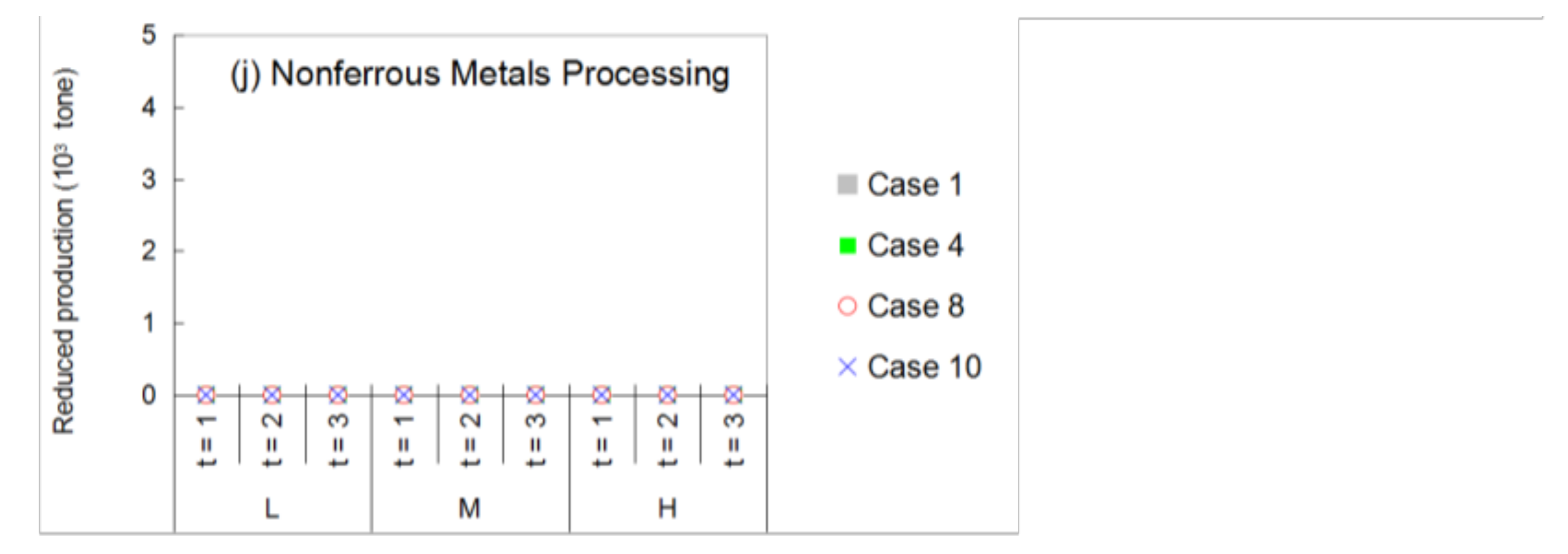
Figure 5 presents excessive PM10 and PM2.5 emissions under cases 1, 4, 8 and 10 when ε and α levels are 0.95 and 0.99, respectively. The highest excess emission PM10 and PM2.5 would occur in progressive plans due to expanding economic development. Although the conservative scenario can reduce the emission of PM10 and PM2.5, lower production would influence the region’s total strategy of urban development. The cases under the Laplace scenario would generate eclectic results among basic plans, progressive water plans and a conservative scenario.
Figure 6 presents the system benefits under cases 1, 5, 7, 9, 10 and an optimal state when α level is varied (ε = 0.95). The results indicate that a lower α level can result in a lower benefit and vice versa. Meanwhile, varied cases can bring about various system benefits as follows: (a) the conservative case (i.e., case 5) can generate lower environmental penalties and retreatment costs, since it require higher environmental protection than economic development; (b) the progressive cases (i.e., cases 7 and 9) can generate the opposite results compared to the conservative cases. Their higher target requirements for the economy would bring about higher environmental penalties; (c) in comparison, the basic case (i.e., case 1) can generate higher benefits than cases 5, 7 and 9. For instance, when α level is 0.9, system benefit would be RMB ¥3.87 × 10¹² under case 1, while system benefits are RMB ¥3.45 × 10⁹ and $1.05 × 10⁹ under case 5 and case 7; (d) the Laplace scenario (case 10) can generate the highest system benefit since it can generate a reliable result according to an element of risk. This implies that the current plan (i.e., case 1) should be adjusted to approach the Laplace scenario (case 10), achieving an optimal state.
5. Discussion
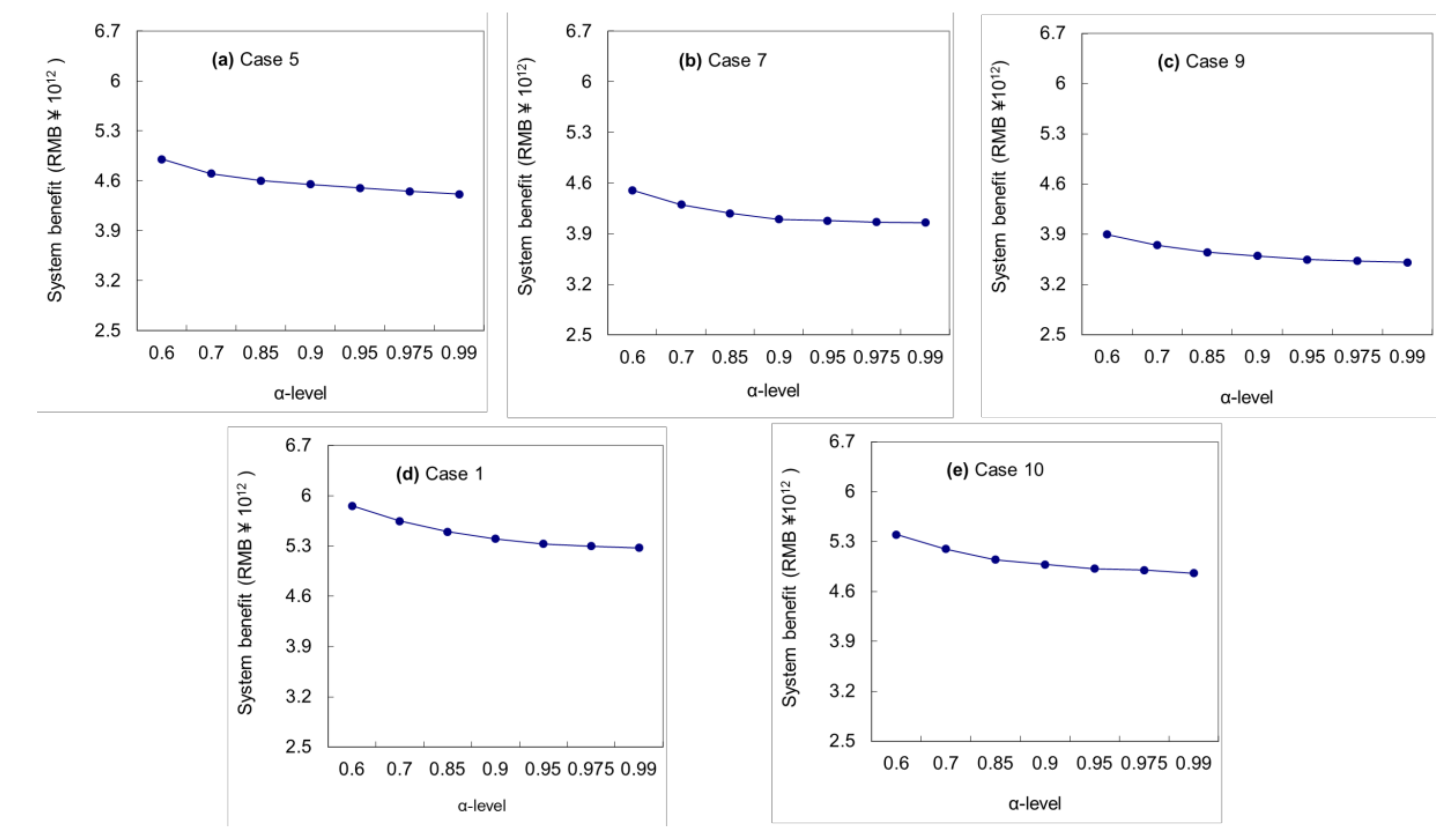
Figure 7 displays the solutions for excessive NO2 emissions under case 1 with trading and non-trading mechanisms when ε and α levels are 0.6 and 0.5, respectively. The results show that a trading-oriented mechanism is superior to non-trading over the planning horizon. In a trading mechanism, an emission permit can be encouraged from low-emission to high-emission industrial sectors. Since a buyer should pay too much money for excessive emissions, the buyer should consider improving the industrial productiveness or retreatment efficiency instead, which can prompt emission mitigation. Under this situation, the pollutant emission under the trading mechanism is lower than that under the non-trading mechanism. For example, the NO2 emissions with the trading scheme would be 157 mg/m3, which is lower than that with the non-trading scheme (197 mg/m3). Under same policy scenario, the trading-oriented mechanism can improve emission mitigation, which can reduce the environmental penalty of excessive pollutant emission, leading to higher system benefits.
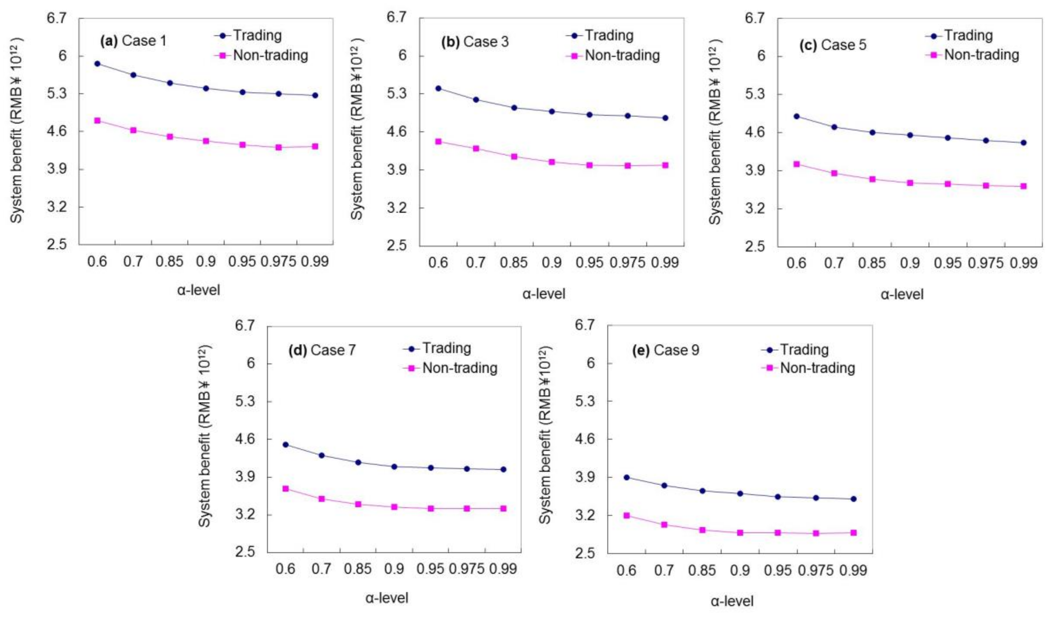
Although a trading mechanism can prompt emission mitigation, reduced production can cut down the economic benefit from industrial sectors. Therefore, the optimized system benefit can be calculated based on the trade-off between an industrial economy and an environmental penalty. Comparing system benefits with trading and non-trading mechanisms, the results show that the trading approach is a more effective method than a non-trading mechanism for an industry-environment plan, which can increase and improve economic returns on the whole (as shown in Figure 8). Emission permits can be encouraged to move from a low value to a high value in a market, which can generate higher benefits than with a non-trading approach. For example, under case 1, when η is 0.9, system benefits would be RMB ¥5.42 × 10¹² with a trading mechanism, while system benefits are RMB ¥4.58 × 10⁹ without a trading approach. Meanwhile, the system benefit can vary with α level.
The results obtained can bring about the following findings: (a) unreasonable industrial structure and excessive production has enhanced the occurrences of hazed air pollution. A laissez-faire policy leading to the overdevelopment of industry would lead to excessive pollutant emissions exceeding the atmospheric load. Therefore, improving the productivities of production and outdated retreatment techniques would aggravate pollution issues. (b) A trading mechanism is a more effective manner of improving the efficiency of pollutant mitigation on the whole. Therefore, improving market construction/market behavior can improve the efficiency of emission permit trading to coordinate industrial production and environmental protection. (c) An unscientific risk choice (including confidence levels and scenario planning) in a decision process with uncertainties can affect an IEST plan, which adversely affects the policymaker leading to neither adventurous nor conservative decisions.
6. Conclusions
In this study, a dual stochastic mixed fuzzy risk analysis method embedded into an optimized industry-environment strategy with an emission-permit trading mechanism (IEST) is proposed for remitting the pressures of frequent/severe haze events in Beijing in conditions of uncertainty. The novelty of the developed method is incorporating TSP, SLC, and FCP into a general framework to deal with multiple formats of uncertainty in a practical IEST issue, which can prompt a capacity to handle complexities and uncertainties. The developed method couples risk analysis, optimization and strategy adjustment into a framework to reflect objective uncertainties (e.g., meteorological conditions, economic development and environmental pollution) regarded as possibility and probability distributions. Meanwhile, it can reflect subjective uncertainties such as the risk attitudes of policymakers in a practical IEST issue. This has assessed the risk based on desired risk exposure level and aspiration benefit level within a two-stage context, with the aim of controlling the environmental penalty in a rational range. Moreover, it can optimize the industry-environment plan with a trading-mechanism, which can prompt pollutant emission from low to high values, encouraging pollutant mitigation.
Although the developed DSFRL method applied to an IEST issue can effectively deal with multiple uncertainties and identify environmental risk under uncertainties. It can help authorities to assess and manage urban environmental risk in order to obtain sustainable industry-environment solutions. However, in an industry-environment system, the environmental loading for various pollutant emissions is difficult to calculate accurately over an extensive area with sporadic time frames. It should take account of various diffusion mechanisms and characterize the spatial and temporal variations of meteorological conditions for emission permit trading. Coupling simulation and a genetic algorithm can reflect, above all, the uncertainties and their interactions in an effective manner in further research.
Acknowledgments
This research was supported by National Social Science Fund (14BFX107), Beijing Social Science Fund (17SRC35) and National Natural Science Fund (51608422). The authors are grateful to the editors and the anonymous reviewers for their insightful comments and suggestions.
Author Contributions
Xueting Zeng conceived and designed the model; Guilin Gao performed the experiments; Chunjiang An contributed modelling calculation; Lei Yu analyzed the result.
Conflicts of Interest
The authors declare no conflicts of interest.
Nomenclature
| Subscript | |
| j | Pollutant emission: j = 1 SO2, j = 2 NO2, j = 3 PM10, j = 4 PM2.5 |
| t | Period: t = 1 period 1, t = 2 period 2, t = 3 period 3 |
| h | Wind velocity level: h = 1 Low, h = 2 Medium, h = 3 High |
| m | Heavy consumption/pollution industry: m = 1 Iron processing, m = 2 Petroleum refining, m = 3 Chemical industry, m = 4 Power generation, m = 5 Heating supply |
| n | Medium consumption/pollution industry: n = 1 Paper-msimilarg industry, n = 2 Cement manufacturing, n = 3 Raw coal processing |
| i | Light consumption/pollution industry: i = 1 Vehicle manufacturing, i = 2 Nonferrous metals processing |
| Notation | |
| , , | production target for heavy/medium/light consumption and pollution industrial activity m/n/i in period t (unit) |
| , , | net benefit for heavy/medium/light consumption and pollution industrial activity m per unit production being generated in period t (RMB ¥/unit) |
| , , | the coefficient of pollution generation for heavy/medium/light consumption and pollution industry activity m/n/i per unit of production being generated in period t |
| the changes of coefficient of pollutant retreatment (%) | |
| , , | loss for heavy/medium/light consumption and pollution industry activity m per unit production being reduced in period t (RMB ¥/unit) |
| , , | reduced production for heavy/medium/light consumption and pollution industry activity m/n/i in period t (person) |
| , , | environmental penalty of excessive emission for heavy/medium/light consumption and pollution industry activity m in period t (RMB ¥/unit) |
| the changes of coefficient of industrial productiveness (%) | |
| , , | retreatment cost for heavy/medium/light consumption and pollution industry activity m per unit of production in period t (RMB ¥/unit) |
| , , | emission-permit transaction for heavy/medium/light consumption and pollution industry activity m per unit of production in period t (tone) |
| , , | net benefit from emission-permit transaction for heavy/medium/light consumption and pollution industry activity m per unit of production in period t (RMB ¥/tone) |
| , , | net trading cost from emission-permit transaction for heavy/medium/light consumption and pollution industry activity m per unit of production in period t (RMB ¥/tone) |
| average efficiencies of retreatment for each pollutant emission j in period t | |
| , , , | pollutant-mitigation requirement for heavy/medium/light consumption and pollution industry activity m/n/i in period t in period t (tone/day) |
| the change of pollutant-mitigation requirement (%) | |
| , , , | maximum pollutant-mitigation capacity for heavy/medium/light consumption and pollution industry activity m/n/i in period t in period t (tone/day) |
| , , , | pollutant-emission allowance for heavy/medium/light consumption and pollution industry activity m/n/i in period t in period t |
| , , , | available emission-permit for trading at the four emission types in period t (µg/m3) |
| , , , | allowance pollutant-loading level at the four emission types in period t (µg/m3) |
| , , , | input pollutant level from nearby regions at the four emission types in period t (µg/m3) |
| , , , | output pollutant level to nearby regions at the four emission types in period t (µg/m3) |
| the probability under scenario h | |
| , | minimum/maximum population growth scale in period t (person) |
| , , , , , , | minimum/maximum industrial production scale in period t (tone) |
| s | wind velocity in period t (m/s) |
| H | the height of pollutant emission diffusion (m) |
| , | the coefficient of standard deviations of the plume at and z directions (m) |
References
- Kathleen, B.A.; Raymond, R.T.; Alvin, B.C.; Jose, B.C. Fuzzy input/output model for optimizing eco-industrial supply chains under water footprint constraints. J. Clean. Prod. 2011, 19, 187–196. [Google Scholar] [CrossRef]
- Jiang, C.; Wang, H.; Zhao, T.; Li, T.; Che, H. Modeling study of PM2.5 pollutant transport across cities in China’s Jing-Jin-Ji region during a severe haze episode December 2013. Atmos. Chem. Phys. 2015, 15, 5803–5814. [Google Scholar] [CrossRef]
- Cheng, Z.; Ma, X.; He, Y.; Jiang, J.; Wang, X.; Wang, Y.; Sheng, L.; Hu, J.; Yan, N. Mass extinction efficiency and extinction hygroscopicity of ambient PM2.5 in urban China. Environ. Res. 2017, 156, 239–246. [Google Scholar] [CrossRef] [PubMed]
- Forster, P.M.F.; Shine, K.P.; Stuber, N. It is premature to include non-CO2 effects of aviation in emission trading schemes. Atmos. Environ. 2006, 40, 1117–1121. [Google Scholar] [CrossRef]
- Clemens, B.; Bamford, C.E.; Douglas, T.J. Choosing strategic responses to address emerging environmental regulations: Size, perceived influence and uncertainty. Bus. Strategy Environ. 2008, 17, 493–511. [Google Scholar] [CrossRef]
- Boldo, E.; Linares, C.; Aragonés, N.; Lumbreras, J.; Borge, R.; de la Paz, D.; Pérez-Gómez, B.; Fernández-Navarro, P.; García-Pérez, J.; Pollán, M.; et al. Air quality modeling and mortality impact of fine particles reduction policies in Spain. Environ. Res. 2014, 128, 15–26. [Google Scholar] [CrossRef] [PubMed]
- ApSimon, H.M.; Warren, R.F.; Kayin, S. Addressing uncertainty in environmental modelling: A case study of integrated assessment of strategies to combat long-range transboundary air pollution. Atmos. Environ. 2002, 36, 5417–5426. [Google Scholar] [CrossRef]
- Scellato, S.; Fortuna, L.; Frasca, M.; Gómez-Gardeñes, J.; Latora, V. Traffic optimization in transport networks based on local routing. Eur. Phys. J. B 2010, 73, 303–308. [Google Scholar] [CrossRef]
- Haar, L.N.; Haar, L. Policy-making under uncertainty: Commentary upon the European Union Emissions Trading Scheme. Energy Policy 2006, 34, 2615–2629. [Google Scholar] [CrossRef]
- Nahorski, Z.; Horabik, J. Compliance and emission trading rules for asymmetric emission uncertainty estimates. Clim. Chang. 2007, 103, 303–325. [Google Scholar] [CrossRef]
- Chen, W.T.; Li, Y.P.; Huang, G.H.; Chen, X.; Li, Y.F. A two-stage inexact-stochastic programming model for planning carbon dioxide emission trading under uncertainty. Appl. Energy 2010, 87, 1033–1047. [Google Scholar] [CrossRef]
- Caponetto, R.; Fortuna, L.; Graziani, S.; Xibilia, M.G. Genetic algorithms and applications in system engineering: A survey. Trans. Inst. Meas. Control 1993, 15, 143–156. [Google Scholar] [CrossRef]
- Weinhofer, G.; Busch, T. Corporate Strategies for Managing Climate Risks. Bus. Strategy Environ. 2013, 22, 121–144. [Google Scholar] [CrossRef]
- Li, Y.P.; Huang, G.H. Interval-parameter two-stage stochastic nonlinear programming for water resources management under uncertainty. Water Resour. Manag. 2008, 22, 681–698. [Google Scholar] [CrossRef]
- Ahmed, S.; Sahinidis, N.V. Robust process planning under uncertainty. Ind. Eng. Chem. Res. 1998, 37, 1883–1892. [Google Scholar] [CrossRef]
- Barbaro, A.; Bagajewicz, M.J. Managing financial risk in planning under uncertainty. AIChE J. 2004, 50, 963–989. [Google Scholar] [CrossRef]
- Peterson, G.D.; Graeme, S.C.; Stephen, R.C. Scenario Planning: A Tool for Conservation in an Uncertain World. Conserv. Biol. 2003, 17, 358–366. [Google Scholar] [CrossRef]
- Zeng, X.T.; Huang, G. A simulation-based resource-environment management model for regional sustainability in compound wetland ecosystem under uncertainties. Ecol. Model. 2016, 334, 60–77. [Google Scholar] [CrossRef]
- Liu, B.; Liu, Y.K. Expected value of fuzzy variable and fuzzy expected value models. IEEE Trans. Fuzzy Syst. 2002, 10, 45–50. [Google Scholar] [CrossRef]
- Inuiguchi, M. Robust optimization by fuzzy linear programming in Managing Safety of Heterogeneous Systems. Lect. Notes Econ. Math. Syst. 2012, 658, 219–239. [Google Scholar] [CrossRef]
- Huang, G.H.; Loucks, D.P. An inexact two-stage stochastic programming model for water resources management under uncertainty. Civil Eng. Environ. Syst. 2000, 17, 95–118. [Google Scholar] [CrossRef]
- Pishvaee, M.S.; Torabi, S.A.; Razmi, J. Credibility-based fuzzy mathematical programming model for green logistics design under uncertainty. Comp. Ind. Eng. 2012, 62, 624–632. [Google Scholar] [CrossRef]
- Swarta, R.J.; Raskinb, P.; Robinsonc, J. The problem of the future: Sustainability science and scenario analysis. Glob. Environ. Chang. 2004, 14, 137–146. [Google Scholar] [CrossRef]
- Beijing Municipal Bureau of Statistics. Beijing Statistical Yearbook (BSY) 2000; Beijing Municipal Bureau of Statistics: Beijing, China, 2001.
- Beijing Municipal Bureau of Statistics. Beijing Statistical Yearbook (BSY) 2013; Beijing Municipal Bureau of Statistics: Beijing, China, 2014.
- Xu, Y.; Huang, G.H. Development of an improved fuzzy robust chance-constrained programming model for air quality management. Environ. Model. Assess. 2015, 20, 535–548. [Google Scholar] [CrossRef]
- Ministry of Environmental Protection. Ambient Air Quality Standard (GB 3095 2012); Ministry of Environmental Protection: Beijing, China, 2012.
- Beijing Municipal Environmental Protection Bureau. Integrated Emission Standards of Air Pollutants (DB11/501 2017); Beijing Municipal Environmental Protection Bureau: Beijing, China, 2017.
Figure 1.
Framework of a risk control-based pollutant emission management model with Laplace’s criterion (RPEL) and its application.
Figure 1.
Framework of a risk control-based pollutant emission management model with Laplace’s criterion (RPEL) and its application.

Figure 2.
Total excess pollution emissions under various cases when ε and α levels are 0.95 and 0.99, respectively (without trading mechanism).
Figure 2.
Total excess pollution emissions under various cases when ε and α levels are 0.95 and 0.99, respectively (without trading mechanism).
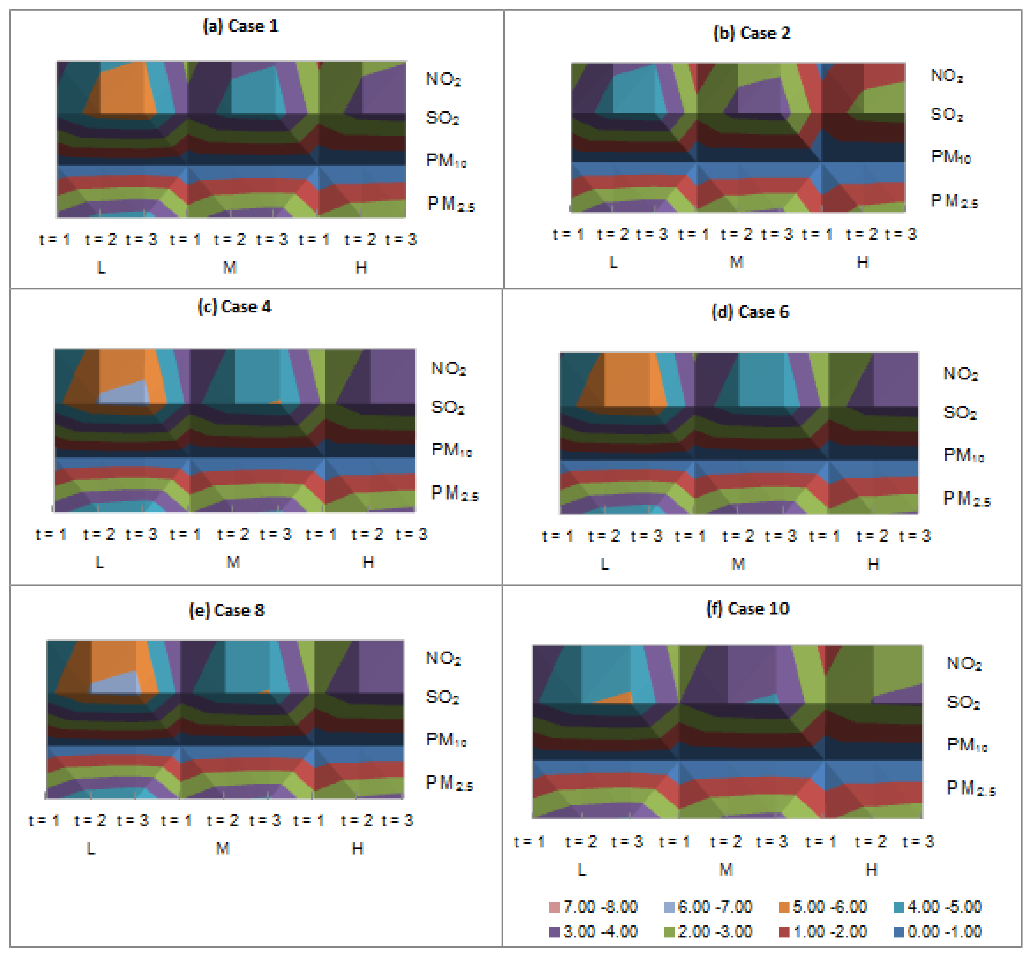
Figure 3.
The transaction of emission permits among various industrial sectors under case 1 when ε and α levels are 0.95 and 0.99, respectively.
Figure 3.
The transaction of emission permits among various industrial sectors under case 1 when ε and α levels are 0.95 and 0.99, respectively.
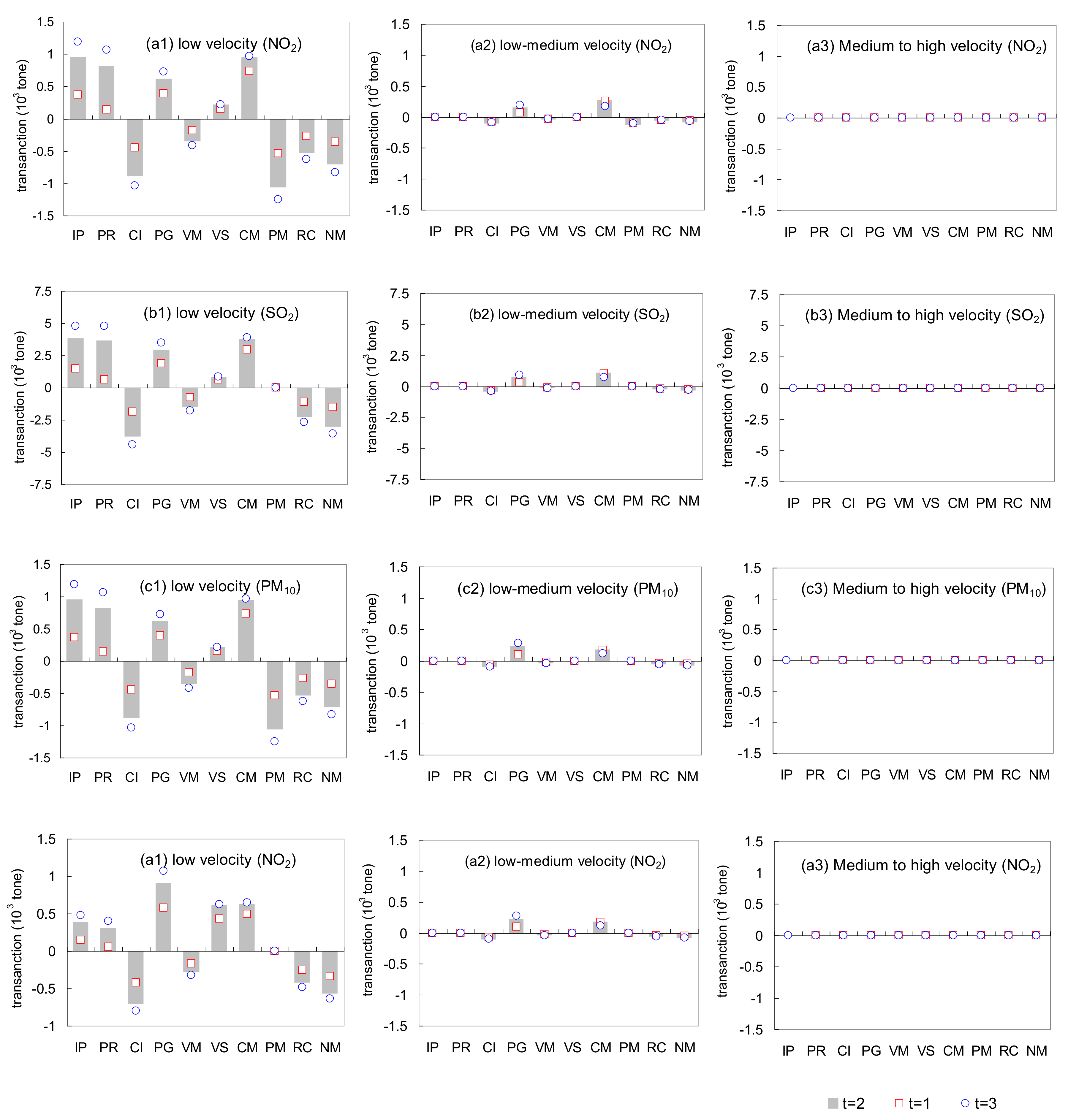
Figure 4.
Optimized reduced production among various industrial sectors under cases 1, 4, 8 and 10 when ε and α levels are 0.95 and 0.99.
Figure 4.
Optimized reduced production among various industrial sectors under cases 1, 4, 8 and 10 when ε and α levels are 0.95 and 0.99.


Figure 5.
Excessive PM10 and PM2.5 emissions under cases 1, 4, 8 and 10 when ε and α levels are 0.95 and 0.99, respectively.
Figure 5.
Excessive PM10 and PM2.5 emissions under cases 1, 4, 8 and 10 when ε and α levels are 0.95 and 0.99, respectively.
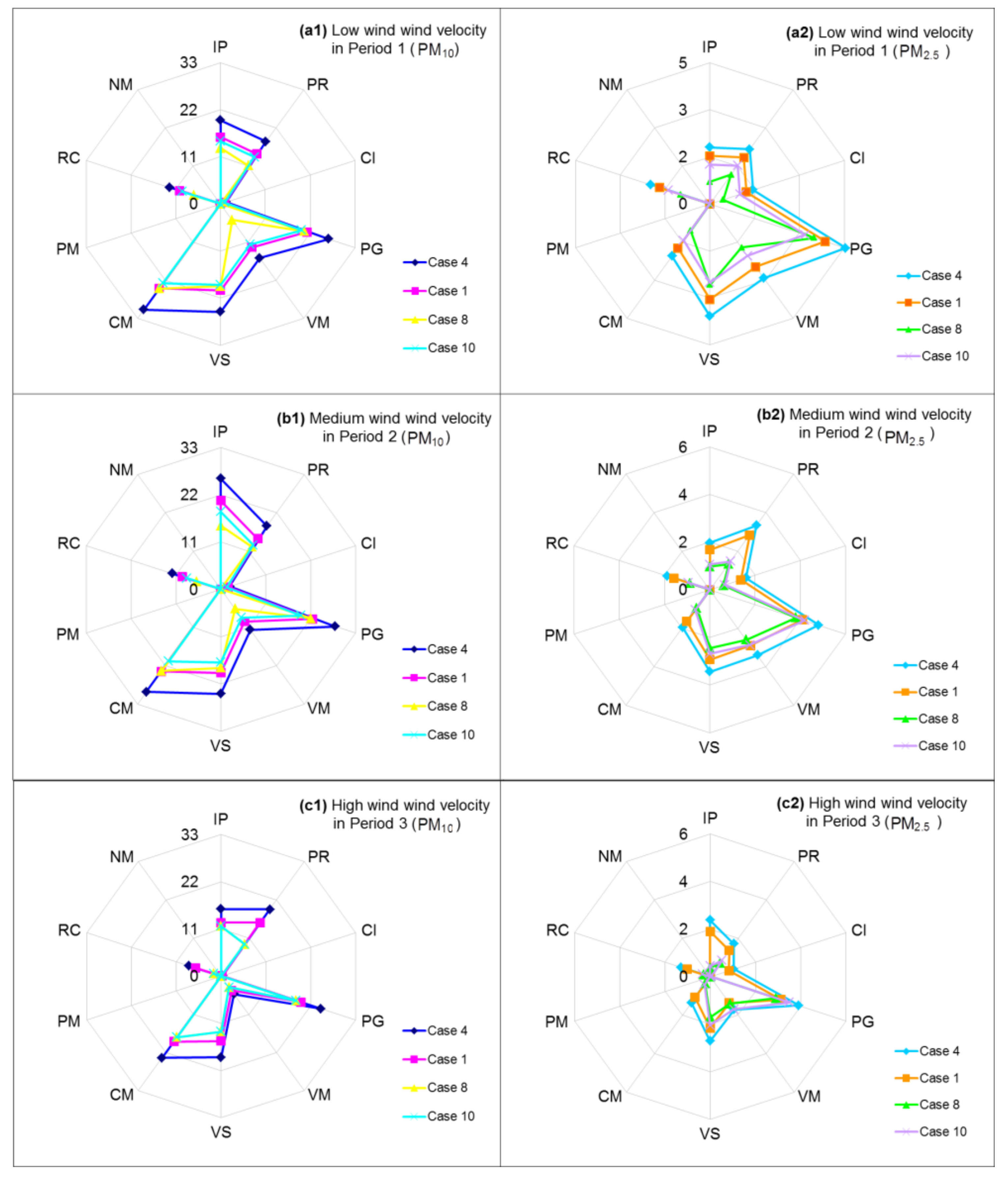
Figure 6.
System benefits under cases 1, 5, 7, 9, 10 and optimal state when α level is varied (ε = 0.95).
Figure 6.
System benefits under cases 1, 5, 7, 9, 10 and optimal state when α level is varied (ε = 0.95).

Figure 7.
Excessive NO2 emissions under various case 1 with trading and non-trading mechanisms when ε and α levels are 0.6 and 0.5, respectively.
Figure 7.
Excessive NO2 emissions under various case 1 with trading and non-trading mechanisms when ε and α levels are 0.6 and 0.5, respectively.

Figure 8.
Excessive NO2 emissions in case 1 with trading and non-trading mechanisms when ε level is 0.5.
Figure 8.
Excessive NO2 emissions in case 1 with trading and non-trading mechanisms when ε level is 0.5.


Table 1.
Economic data.
| Industrial Activities | Planning Period | ||
|---|---|---|---|
| t = 1 | t = 2 | t = 3 | |
| Net system benefit for industrial activities | |||
| Iron processing (103 RMB ¥/tonne) | 13.55 | 14.97 | 16.32 |
| Petroleum refining (103 RMB ¥/tonne) | 6.55 | 7.21 | 7.62 |
| Chemical industry (103 RMB ¥/tonne) | 2.06 | 2.82 | 3.07 |
| Power generation (103 RMB ¥/106 kWh) | 0.88 | 0.97 | 1.11 |
| Vehicle manufacturing (103 RMB ¥/car) | 13.72 | 14.21 | 14,84 |
| Heating supply (103 RMB ¥/106 kj) | 0.32 | 0.39 | 0.59 |
| Cement manufacturing (103 RMB ¥/tonne) | 0.38 | 0.43 | 0.51 |
| Paper-making industry (103 RMB ¥/tonne) | 3.23 | 3.57 | 3.81 |
| Raw cow processing (103 RMB ¥/tonne) | 0.45 | 0.58 | 0.69 |
| Non-ferrous metal processing (103 RMB ¥/tonne) | 9.00 | 9.56 | 9.91 |
| Penalty for excess emission of unit production | |||
| Iron processing (103 RMB ¥/tonne) | 15.55 | 16.97 | 18.32 |
| Petroleum refining (103 RMB ¥/tonne) | 7.55 | 8.21 | 8.62 |
| Chemical industry (103 RMB ¥/tonne) | 2.46 | 3.12 | 3.77 |
| Power generation (103 RMB ¥/106 kWh) | 0.98 | 1.27 | 1.81 |
| Vehicle manufacturing (103 RMB ¥/car) | 15.72 | 16.21 | 16,84 |
| Heating supply (103 RMB ¥/106 kj) | 0.42 | 0.49 | 0.69 |
| Cement manufacturing (103 RMB ¥/tonne) | 0.52 | 0.65 | 0.77 |
| Paper-making industry (103 RMB ¥/tonne) | 4.23 | 4.57 | 4.81 |
| Raw cow processing (103 RMB ¥/tonne) | 0.51 | 0.68 | 0.79 |
| Non-ferrous metal processing (103 RMB ¥/tonne) | 9.78 | 10.46 | 9.90 |
Table 2.
The meteorological data.
| Level of Wind Velocity | Probability (%) | Velocity | ||
|---|---|---|---|---|
| t = 1 | t = 2 | t = 3 | ||
| L | 0.3 | (2.22, 2.46, 2.52) | (2.55, 2.53, 2.62) | (2 63, 2.74, 2.92) |
| M | 0.5 | (2.97, 3.06, 3.19) | (3.26, 3.35, 3.93) | (3.95, 4.19, 4.29) |
| H | 0.2 | (4.22, 4.36, 4.47) | (4.53, 4.62, 4.72) | (4.80, 4.99, 5.13) |
Table 3.
List of scenarios.
| Abbreviation | Scheme | |
|---|---|---|
| Case1 | Basic scenario | Expected industrial development target equal to current plan. |
| Case 2 | Conservative scenario | Expected industrial development target is 3% lower than the need of economic development to accommodate the environment |
| Case 3 | Expected industrial development target is 5% lower than the need of economic development to accommodate the environment | |
| Case 4 | Expected industrial development target is 8% lower than the need of economic development to accommodate the environment | |
| Case 5 | Expected industrial development target is 10% lower than the need of economic development to accommodate the environment | |
| Case 6 | Progressive scenario | Expected industrial development target is increased by the speed of economic development (3%) absolutely |
| Case 7 | Expected industrial development target is increased by the speed of economic development (5%) absolutely | |
| Case 8 | Expected industrial development target is increased by the speed of economic development (8%) absolutely | |
| Case 9 | Expected industrial development target is increased by the speed of economic development (10%) absolutely | |
| Case 10 | Laplace scenario | Expected industrial development target is calculated according to Laplace criterion. |
© 2018 by the authors. Licensee MDPI, Basel, Switzerland. This article is an open access article distributed under the terms and conditions of the Creative Commons Attribution (CC BY) license (http://creativecommons.org/licenses/by/4.0/).
Share and Cite
MDPI and ACS Style
Gao, G.; Zeng, X.; An, C.; Yu, L. A Sustainable Industry-Environment Model for the Identification of Urban Environmental Risk to Confront Air Pollution in Beijing, China. Sustainability 2018, 10, 962. https://doi.org/10.3390/su10040962
AMA Style
Gao G, Zeng X, An C, Yu L. A Sustainable Industry-Environment Model for the Identification of Urban Environmental Risk to Confront Air Pollution in Beijing, China. Sustainability. 2018; 10(4):962. https://doi.org/10.3390/su10040962
Chicago/Turabian StyleGao, Guilin, Xueting Zeng, Chunjiang An, and Lei Yu. 2018. "A Sustainable Industry-Environment Model for the Identification of Urban Environmental Risk to Confront Air Pollution in Beijing, China" Sustainability 10, no. 4: 962. https://doi.org/10.3390/su10040962
Note that from the first issue of 2016, this journal uses article numbers instead of page numbers. See further details here.