R&D Project Valuation Considering Changes of Economic Environment: A Case of a Pharmaceutical R&D Project

Abstract

R&D project valuation is important for effective R&D portfolio management through decision making, related to the firm’s R&D productivity, sustainable management. In particular, scholars have emphasized the necessities of capturing option value in R&D and developed methods of real option valuation. However, despite suggesting various real option models, there are few studies on simultaneously employing mean-reverting stochastic process and Markov regime switching to describe the evolution of cash flow and to reflect time-varying parameters resulting from changes of economic environment. Therefore, we suggest a mean-reverting binomial lattice model under Markov regime switching and apply it to evaluate clinical development with project cases of the pharmaceutical industry. This study finds that decision making can be different according to the regime condition, thus the suggested model can capture risks caused by the uncertainty of the economic environment, represented by regime switching. Further, this study simulates the model according to rate parameter from 0.00 to 1.00 and risk-free interest rates for regimes 1 and 2 from ($r_1$ = 4%, $r_2$ = 2%) to ($r_1$ = 7%, $r_2$ = 5%), and confirms the rigidity of the model. Therefore, in practice, the mean-reverting binomial lattice model under Markov regime switching proposed in this study for R&D project valuation contributes to assisting company R&D project managers make effective decision making considering current economic environment and future changes.

1. Introduction

R&D portfolio management facilitates decision-making on project selection and the prioritization and allocation of resources for project progression [1,2,3]. Decision-making on R&D portfolio management is based on an economic valuation of firm R&D projects. Therefore, valuation of R&D projects is a critical factor for enhancing a firm’s efficiency and towing its growth, which means that it can be a tool of sustainable management. Various methods of R&D project valuation have been introduced so far.

Previous studies on the valuation of R&D projects are largely divided into two categories: one is the discounted cash flow (DCF) analysis, often called the expected net present value or risk-adjusted net present value [4], and the other is the real options valuation (ROV) analysis, which adopts the financial option pricing method.

In particular, the ROV can be a strategic device to capitalize on upside potential and mitigate downside risks [5]. The risk is an especially key issue for managers and investors. The ROV is useful for the risk analysis of various projects with managerial flexibility [6,7]. The ROV has highlighted sustainable management to properly realign the firm’s strategies according to risks from uncertainties related with the business environment [8,9]. Scholars proposed a binomial lattice model [10,11,12], option models compounding Geske’s and the fuzzy model [13,14], the Monte Carlo simulation (MCS) approach with general stochastic processes and assumption of sales of a drug governed by a mean-reverting stochastic process [15,16,17], and the mean-reverting binomial lattice model [18] for the valuation of R&D projects in various industries.

However, most ROV models proposed in previous studies assume that model parameters such as market volatility and risk-free interest rates are constant throughout the project period, but this assumption should be considered as time-varying parameters. The valuation result of the ROV is likely to go wrong unless its underlying assumptions are consistent with reality [19]. Few studies have proposed a more realistic ROV model to encourage the decision making of the firm. To this fashion, Markov regime switching may be a useful approach to accommodate the time-varying aspect of parameters in ROV models [20,21,22]. Therefore, we suggest the valuation method with mean-reverting binomial lattice model under Markov regime switching. Then, this study compares valuation results from the proposed model with those from conventional DCF and previous ROV models and performs a sensitivity analysis regarding the major parameters of the model.

The focus of this study is the valuation of R&D projects in the pharmaceutical industry. Pharmaceutical R&D projects have characteristics of the long period of the R&D process and tremendous R&D investment, thus a high uncertainty of R&D success. Generally, it takes approximately 10 to 12 years to develop a new drug from discovery to commercialization [23], and the total R&D budget for a new drug often exceeds $1 billion USD [24]. These features make an accurate valuation of pharmaceutical R&D projects considering risks critical for a firm’s decision makers related to its sustainable development.

Previous studies on the valuation of pharmaceutical R&D projects are largely divided into two categories: one is DCF analysis, often called the expected net present value or risk-adjusted net present value [4], and the other is ROV analysis, which adopts the financial option pricing method. In particular, ROV has highlighted dealing with managerial flexibility around issues such as economically motivated abandonment, expansion, and contraction of R&D investments. It also considers the uncertainty of market potential [8,9]. Kellogg and Charnes [10], Bogdan and Villiger [11], and Hauschild and Reimsbach [12] proposed a binomial lattice model for the evaluation of a clinical drug development project. Cassimon et al. [13] and Wang and Hwang [14] suggested a generalized version of Geske’s compound option model and the fuzzy compound option model to evaluate a new drug development project. They considered each phase of drug development as a compound option and solved the model with the partial differential equation approach, which was quite complex. They also assumed that the cash flow from sales of a drug is governed by a geometric Brownian motion (GBM), which is rather unrealistic. A mean-reverting process is the most often-used assumption concerning the cash flow of a project in ROV models [18,25,26]. Myers and Howe [15] and Schwartz [16] proposed an MCS approach, which can easily model general stochastic processes. Willigers and Hansen [17] strengthened the MCS approach by adding the assumption that the logarithm of sales of a drug is governed by a mean-reverting stochastic process, which is closer to reality. However, the MCS approach is computationally intensive and complex compared to a lattice-based model.

Our proposed real option valuation model in this study contributes to helping decision makers consider the changes of economic environment and the adequate future cash flows estimation of R&D projects. Most ROV models previously proposed in the pharmaceutical industry assume that model parameters such as market volatility and risk-free interest rates are constant throughout the project development period, but this assumption is somewhat unrealistic considering the long span of pharmaceutical R&D projects. The valuation result of the ROV is likely to go wrong unless its underlying assumptions are consistent with reality [19]. We propose a new real option valuation model which simultaneously employs mean-reverting stochastic process and time-varying parameters based on a binomial lattice approach. The mean-reversion assumption and a regime switching technique can more realistically capture the characteristics of R&D projects and the structural changes of economic conditions [17,27]. Additionally, as Mun [28] indicated, a lattice-based approach is relatively intuitive and can therefore be accepted easily. Therefore, this study contributes to the effective decision making of pharmaceutical companies, to find more accurate and intuitive valuations of R&D projects.

The rest of this study is organized into four sections. In Section 2, we introduce the process of drug development and risks involved, and we then present our proposed economic valuation model. We describe data and assumptions used in the valuation in Section 3, which is followed by the presentation of valuation results and discussions in Section 4. Finally, in Section 5, we conclude the study with the implications, limitations, and future research of the study.

2. Background and Development of Model

2.1. Development of a New Drug and Risks in Pharmaceutical Industry

Bringing a new drug from laboratories to markets largely consists of three stages: discovery, development, and commercialization. New chemical entities (NCEs) or new molecular entities for a disease target are found through target identification, target validation, lead generation, and lead optimization in the discovery stage, which is followed by preclinical studies, Phases I through III clinical trials, registration, and launching in the development and commercialization stages. Toxicity and pharmacological activities of the selected NCEs are tested in animals in preclinical trials before trials in humans. With successful results from the preclinical study, a pharmaceutical company applies for investigational new drug (IND) approval from regulatory bodies such as the Food and Drug Administration (FDA) in the U.S., which is required to move forward to clinical development with human subjects [29]. Phase I of clinical development mostly investigates safety issues with a small group of healthy human volunteers [10]. Efficacy studies start at the Phase II trials on a larger number of patients, usually less than 300, with the target disease and the IND. The IND should demonstrate distinct efficacy, which is its most important value driver. Phase III trials are multicenter trials with a much larger number of target patients to study the IND’s effectiveness, as well as additional information regarding side effects and dosage [11]. After the successful completion of clinical trials, a pharmaceutical company is ready to file a new drug application and submit all findings from previous studies to the regulatory body for a new drug approval. If the registration with the regulatory body, such as the FDA in the U.S., is successful, the new drug is prepared for launching when the regulatory body reviews the application and grants approval.

There are two types of risks involved in the development and commercialization of a new drug: technical risks and market risks. Technical risks are associated with uncertainties as to the technological aspects of drugs. Examples of such uncertainties include failures in phases of the drug’s development and unanticipated toxicity and side effects found after launch that result in withdrawal of the drug from the market. DiMasi et al. [23] reported that only one out of six new drug developments that enter clinical studies yield a marketable drug. Market risks and uncertainties are associated with commercial potentials, which are affected by the size of the population with the target disease, new competing drugs entering the market, third party payer’s payment regulations, and the economy in general [17,30].

2.2. Mean-Reverting Binomial Lattice Model

The GBM is the most frequently used stochastic process in the financial option pricing and ROV. Cash flows are assumed to be log-normally distributed in a GBM. However, historical data indicates that the financial outcomes measured, such as commodity price and company earnings, are more likely to be governed by a mean-reverting stochastic process rather than a GBM [26,31,32]. While a GBM generates extreme cash flows near the expiration when compared to initial cash flows, the market size of a specific drug is governed by the number of patients with the target disease throughout the lifecycle of a drug [17]. In our study, the underlying asset is a project of new drug development and its value is total future cash flows. We used a standard sales curve expressed as a percentage of peak sales to estimate the total future sales. Thus, total future sales are determined by peak sales. Therefore, we assume that peak sales of a drug are log-normally distributed and governed by a mean-reverting stochastic process. Next, we can write one-factor mean-reverting stochastic process for the peak sales as Equation (1) [33].

$$d{X}_t=\eta (\ln \overline{X}-\ln X_t)X_{t}dt+\sigma X_{t}d{W}_t,$$

(1)

where $X_t$ = the peak sales of a drug at time t, $\eta$ = the speed of sales reversion, $\overline{X}$ = the long-term mean of the peak sales, $\sigma$ = the standard deviation of the peak sales, and $d{W}_t$ = the increment of Brownian motion.

$X_t$ tends to revert to $\overline{X}$, and $\sigma$ may be interpreted as instantaneous volatility of the peak sales. $\eta$ indicates how quickly the sales converges to the long-term mean level of sales. Equation (1) is rewritten as Equation (2) by substituting $x_t=\ln X_t$ and $\overline{x}=\ln \overline{X}$, and applying the Itō–Doeblin theorem to Equation (1), which shows that the logarithm of peak sales is governed by a simple Ornstein-Uhlenbeck type mean-reverting stochastic process.

$$d{x}_t=\eta (\alpha -x_t)dt+\sigma d{W}_t,$$

(2)

$$\alpha =\overline{x}-\frac{{\sigma }^2}{2\eta },$$

(3)

where $\alpha$ = the adjusted long-term mean of the logarithm of the peak sales.

The expected value and the variance of x at time t can be written as Equations (4) and (5), where the current value of x is $x_0$ [34].

$$E[x_t]=\alpha +(x_0-\alpha )e^{-\eta t},$$

(4)

$$Var[x_t]=\frac{{\sigma }^2}{2\eta }(1-e^{-2\eta t}).$$

(5)

Equations (2)–(5) indicate that when the logarithm of peak sales x deviates from $\alpha$, it is likely to revert to and approach $\alpha$ over the next time period. If $\eta$ approaches positive infinity, then $Var[x_t]$ converges to zero; x does not deviate from $\alpha$. On the other hand, if $\eta$ approaches zero, then x is governed by a simple Brownian motion.

Nelson and Ramaswamy [35] developed a recombining binomial lattice model to solve the general stochastic differential Equation (6). They also applied the approach to a one-factor mean-reverting stochastic problem.

$$d{x}_t=\mu (x,t)dt+\sigma (x,t)d{W}_t,$$

(6)

where $\mu (x,t)$ = the instantaneous mean of return, and $\sigma (x,t)$ = the standard deviation of return.

Let ${\pi }_{tu}$ and ${\pi }_{td}$ be the probabilities of up and down movements of the logarithm of peak sales at a given time t. Figure 1 depicts the basic building block of the binomial lattice proposed by Nelson and Ramaswamy [35] based on Cox and Rubinstein [36].

When the standard deviation $\sigma (x,t)$ is state-dependent, the model becomes complex and the binomial lattice is not recombinant. However, we can obtain simplicity with the assumption that $\sigma (x,t)$ is constant. Nelson and Ramaswamy [35] showed that with that assumption, the binomial lattice presented in Figure 1 is governed by Equations (7)–(10).

$$x_t^{+}\equiv x+\sigma \sqrt{\Delta t},$$

(7)

$$x_t^{-}\equiv x-\sigma \sqrt{\Delta t},$$

(8)

$${\pi }_{tu}\equiv \{\begin{array}{ll}\frac{1}{2}+\frac{1}{2\sigma }\sqrt{\Delta t}\left(\eta (\overline{x}-x_t)-\frac{{\sigma }^2}{2}\right)& \mathrm{if}0\le \frac{1}{2}+\frac{1}{2\sigma }\sqrt{\Delta t}\left(\eta (\overline{x}-x_t)-\frac{{\sigma }^2}{2}\right)\le 1,\\ 0& \mathrm{if}\frac{1}{2}+\frac{1}{2\sigma }\sqrt{\Delta t}\left(\eta (\overline{x}-x_t)-\frac{{\sigma }^2}{2}\right)\le 0,\\ 1& \mathrm{if}1\le \frac{1}{2}+\frac{1}{2\sigma }\sqrt{\Delta t}\left(\eta (\overline{x}-x_t)-\frac{{\sigma }^2}{2}\right).\end{array}$$

(9)

$${\pi }_{td}\equiv 1-{\pi }_{tu},$$

(10)

2.3. Mean-Reverting Binomial Lattice Model under Markov Regime Switching

The time-varying aspect of the economic environment is not modeled in the mean-reverting binomial lattice model presented in Equations (7)–(10). We apply the Markov regime switching approach to the mean-reverting model to incorporate the time-varying aspect in the model. The pattern of drug sales may change to a different pattern during the marketing period because of changes in the market environment, such as newly introduced regulation and payment policies and the market entry of a new competing drug. Volatility of sales, speed of sales reversion, and risk-free interest may also change under the influence of the drug market and the economy in general. The regime refers to the economic environment, and the project value is affected by regimes during the marketing period. In our model, a regime is represented by volatility, the speed of sales reversion, the long-term mean of peak sales, and risk-free interest rates. Accordingly, our model can consider risks due to the changes of economic environment during the long period of drug development and commercialization in the valuation of a drug development project.

We assume that there are k regimes and each regime has a different volatility, speed of reversion, long-term mean of peak sales, and risk-free interest rates, such as $({\sigma }_1,{\eta }_1,{\overline{x}}_1,r_1)$, $({\sigma }_2,{\eta }_2,{\overline{x}}_2,r_2)$, …, $({\sigma }_k,{\eta }_k,{\overline{x}}_k,r_k)$. The regime switching is governed by a Markov process, which is represented by one-step transition probabilities. If the lattice is non-recombinant, it becomes rapidly complex as the number of regimes increases. Thus, we applied the recombining scheme to the model to maintain its simplicity. We assume that the logarithm of the peak sales changes by $\sigma \sqrt{\Delta t}$ during the time interval $\Delta t$, which is applied to all regimes. Haahtela [37] suggested that $\sigma$ should be between ${\sigma }_{\max }$ and $\sqrt{1.5}{\sigma }_{\max }$, where ${\sigma }_{\max }=\underset{1\le i\le k}{\max }{\sigma }_i$, to obtain proper up and down movement probabilities. Therefore, $\sqrt{1.5}{\sigma }_{\max }$ is the upper limit for $\sigma$, and we use Equation (11) to choose $\sigma$, which was suggested by Yuen and Yang [20]. An alternative choice for $\overline{\sigma }$ can be the root mean square of each regime’s volatility, ${\sigma }_i$, for 1 ≤ i ≤ k.

$$\sigma =\underset{1\le i\le k}{\max }{\sigma }_i+(\sqrt{1.5}-1)\overline{\sigma },$$

(11)

where $\overline{\sigma }$ is the arithmetic mean of ${\sigma }_i$.

Let ${\pi }_{tu}^i$ and ${\pi }_{td}^i$ denote the probabilities of up and down movement of the logarithm of peak sales at time t in regime i. We can specify Equations (12) and (13) for ${\pi }_{tu}^i$ and ${\pi }_{td}^i$, and they can be obtained by solving Equations (12) and (13) simultaneously. Equation (14) shows ${\pi }_{tu}^i$, and reveals that the probability of upward movements depends on ${\sigma }_i$, ${\eta }_i$, and ${\overline{x}}_i$, which are governed by a Markov process.

$${\pi }_{tu}^i+{\pi }_{td}^i=1,$$

(12)

$${\pi }_{tu}^i\left(x+\sigma \sqrt{\Delta t}\right)+{\pi }_{td}^i\left(x-\sigma \sqrt{\Delta t}\right)=x+{\mu }_i(x,t)\Delta t,$$

(13)

where ${\mu }_i(x,t)={\eta }_i({\overline{x}}_i-x_t)-({\sigma }_i^2/2)$.

$${\pi }_{tu}^i\equiv \{\begin{array}{ll}\frac{1}{2}+\frac{1}{2\sigma }\sqrt{\Delta t}\left({\eta }_i({\overline{x}}_i-x_t)-\frac{{\sigma }_i^2}{2}\right)& \mathrm{if}0\le \frac{1}{2}+\frac{1}{2\sigma }\sqrt{\Delta t}\left({\eta }_i({\overline{x}}_i-x_t)-\frac{{\sigma }_i^2}{2}\right)\le 1,\\ 0& \mathrm{if}\frac{1}{2}+\frac{1}{2\sigma }\sqrt{\Delta t}\left({\eta }_i({\overline{x}}_i-x_t)-\frac{{\sigma }_i^2}{2}\right)\le 0,\\ 1& \mathrm{if}1\le \frac{1}{2}+\frac{1}{2\sigma }\sqrt{\Delta t}\left({\eta }_i({\overline{x}}_i-x_t)-\frac{{\sigma }_i^2}{2}\right).\end{array}$$

(14)

In a Markov process, the process switches from one regime state to the other in a fixed time interval with a transition probability. Transition probabilities of a Markov process can be calculated with Equation (15) using a generator matrix, A, shown in Equation (16) for the k-regime setup.

$$P(\Delta t)=\left(\begin{array}{cccc}{p}_{11}(\Delta t)& p_{12}(\Delta t)& \dots & p_{1k}(\Delta t)\\ p_{21}(\Delta t)& p_{22}(\Delta t)& \dots & p_{2k}(\Delta t)\\ ⋮& ⋮& \ddots & ⋮\\ p_{k1}(\Delta t)& p_{k2}(\Delta t)& \dots & p_{kk}(\Delta t)\end{array}\right)=e^{A\Delta t}=I+{\displaystyle \sum _{l=1}^{\infty }\frac{{(\Delta t)}^l{A}^l}{l!}}.$$

(15)

$$A=\left(\begin{array}{cccc}{a}_{11}& a_{12}& \dots & a_{1k}\\ a_{21}& a_{22}& \dots & a_{1k}\\ ⋮& ⋮& \ddots & ⋮\\ a_{k1}& a_{k2}& \dots & a_{kk}\end{array}\right),$$

(16)

where $a_{ii}=-{\displaystyle {\sum }_{j=0,j\ne i}^k{a}_{ij}},\mathrm{for}i=0,1,\dots ,k.$ $P(\Delta t)$ = transition probability matrix, and $p_{ij}(\Delta t)$ = probability of transition from regime 1 to regime 2.

Transition probabilities are independent of the probabilities of up and down movements because the Markov process of the regime switching and the mean-reverting stochastic process for peak sales are unrelated to each other. The suggested model approaches a stochastic volatility model when the number of regime states increases and transition probabilities are properly selected [38]. Figure 2 depicts the state diagram of a Markov process with two regimes.

2.4. Technical Risk and Valuation

We assume that the duration of a drug development project from the Phase I clinical trial to the registration with a regulatory body is T and the number of project valuations during that time period is N. Thus, $\Delta t=T/N$ and the number of nodes at the tth valuation is t + 1. Let $V_{t,n,i}$, for i = 1, 2, …, k, denote the adjacent option value of the project at the tth valuation at the nth node in regime i. Thus, $V_{N,n,i}$ is the value of the project at the time of launch, which is at the completion of the registration at the nth node in regime i and is the sum of discounted future cash flows after launch. The cash flows consist of sales of the launched drug, launch costs, and sales costs. We can compute the adjacent option values at the tth valuation with Equation (17).

$$V_{t,n,i}=e^{-r_i\Delta t}\left\{{\displaystyle \sum _{j=1}^k{p}_{ij}(\Delta t)(}{\pi }_{tu}^i{V}_{t+1,n+1,j}+{\pi }_{td}^i{V}_{t+1,n,j})\right\},$$

(17)

We assume that the decision to keep or abandon the project takes place at the start of each development stage and that the technical risk of stage failure is also applied at the start of each development stage. Decision nodes of each development stage s are represented by s = 1, 2, 3, and 4 for Phases I, II, III, and registration, respectively. The option value, $V_{t,n,i}$, is recalculated with Equation (18) to include the development costs and technical risk in the model.

$$V_{t,n,i}=\max \left[(S{R}_s{V}_{t,n,i}-I_s),0\right],$$

(18)

where t = number of evaluations up to the start of the development stage s, $I_s$ = discounted development cost of the development stage s, and $S{R}_s$ = success rate of the development stage s.

Equation (18) indicates that the project is abandoned and the option value becomes zero when the payoff at each decision node falls below zero. The final option values of an R&D project are obtained by recursive backwardation of Equations (17) and (18) up to the start node of the Phase I clinical trial.

3. Evaluation of Model

We applied the mean-reverting binomial lattice model under Markov regime switching (MRBL-MRS) proposed in this study to the clinical development of new drugs in order to assess differences between the valuation resulting from our proposed model and those resulting from other methods proposed by previous studies: conventional DCF, Monte Carlo simulation with GBM (MCS-GBM), Monte Carlo simulation with mean-reverting process (MCS-MRP), binomial lattice model with GBM (BL-GBM), and binomial lattice model with mean-reverting process (BL-MRP) [10,11,12,15,17,18]. We defined five clinical development projects which have different project parameters and assumptions.

3.1. Model Parameters and Assumptions

We assumed that option values of a project are evaluated every quarter during the duration of the development project, and decisions are made at the start of each development stage: Phases I, II, and III, and registration. A decision can be made to either abandon or keep the project. The abandon option is taken when the value of the project at a decision node is negative. Figure 3 illustrates a binomial lattice for the logarithm of peak sales during clinical trials and registration.

The parameter required in the GBM model is volatility, and the mean-reverting model requires three parameters: (1) volatility, (2) speed of sales reversion, and (3) long-term mean of peak sales ratio. We estimated the parameters for the model evaluation using daily data from the Arca Pharmaceutical Index, a weighted index of market-capitalization of highly capitalized global pharmaceutical companies such as Johnson & Johnson, Novartis, Pfizer, GlaxoSmithKline, and Merck. It is often assumed to represent characteristics of company cash flows in the pharmaceutical industry [17]. We assumed that characteristics of changes in drug sales would be reflected in the characteristics of company cash flows. We used daily data from the Arca Pharmaceutical Index from January 2005 to December 2007 to estimate the parameters for the GBM, mean-reverting process, and regime 1 of MRBL-MRS. We used data from June 1998 to May 2001 and from January 2008 to December 2010 for the parameters of regime 2 for MRBL-MRS [39].

Table 1. Parameters of different stochastic processes.

Parameter	GBM	Mean-Reverting Process	MRBL-MRS
			Regime 1	Regime 2
Volatility ($\sigma$)	0.22	0.22	0.15	0.33
Speed of reversion ($\eta$)	-	2.74	5.30	5.43
Long-term mean to initial peak sales ratio ($\overline{X}/X_0$)	-	1.03	1.12	0.91

shows the values of parameters for different stochastic processes used in the evaluation, and details of the estimation are presented in Appendix A and

Table A1. Regression results.

Parameter	Mean-Reverting Process with Regime Switching
	Regime 1	Regime 2
${\beta }_0$	0.164 ***	0.149 ***
${\beta }_1$	0.972 ***	0.976 ***
${\sigma }_{\epsilon }$	0.008	0.017

*** p < 0.01, ** p < 0.05, * p < 0.1.

.

Let $\lambda$ denote the rate parameter which characterizes the Markov process. In the two-regime setup, we can take the generator matrix, such as Equation (19), according to Equation (15).

$$A=\left(\begin{array}{cc}-\lambda & \lambda \\ \lambda & -\lambda \end{array}\right),$$

(19)

The generator matrix and transition probability matrix of the Markov regime switching are assumed to be:

$$A=\left(\begin{array}{cc}-0.1& 0.1\\ 0.1& -0.1\end{array}\right),P(\Delta t)=\left(\begin{array}{cc}0.976& 0.024\\ 0.024& 0.976\end{array}\right).$$

3.2. Project Parameters and Assumptions

Parameters of clinical development projects for a new drug used in the model evaluation were obtained from previous studies presented in

Table 2. Project parameters and sources of data.

Parameter	Source
Development time in each stage	DiMasi, Hansen and Grabowski [41]
Development cost of each stage	DiMasi, Hansen and Grabowski [41]
Success rate of each stage	DiMasi, Feldman, Seckler and Wilson [23]
Cost of launching	Willigers and Hansen [17]
Peak gross sales	DiMasi, Grabowski and Vernon [42]
Sales pattern during the drug life time after launch	Bogdan and Villiger [11]
Sales margin	Bogdan and Villiger [11]
Probability of drug withdrawal from market after launch	Qureshi, Seoane-Vazquez, Rodriguez-Monguio, Stevenson and Szeinbach [40]
Mean time to drug withdrawal from market after launch	Qureshi, Seoane-Vazquez, Rodriguez-Monguio, Stevenson and Szeinbach [40]

. The costs of launching include expenses for acquiring drug production capabilities and organizing and running pre-launch marketing teams. We assumed that the launch costs occur for three years, one year before launch and two years after launch. The effective patent term is given for 20 years, and the patent of a drug therefore expires approximately 12 years after launch, considering the time taken for development. Sales of a drug dramatically diminish after the patent’s expiration when generics enter the market, and eventually dissipate after 22 years after the launch [11]. We assumed that the sales pattern of a drug takes a standard sales curve, and Figure 4 shows the pattern during the 22-year period of marketing represented as a percentage of the peak sales used in the model evaluation. We adjusted the project valuation for the possibility of the drug’s withdrawal from the market, caused by unexpected adverse effects found after the launch. We made the adjustment after six years from the launch, which is the mean time to drug withdrawal from launch, as suggested by Qureshi, et al. [40]. We converted all costs and sales to 2010 US dollars using the US gross domestic product implicit price deflator.

We set up five projects using parameters obtained from the literature presented in Table 2 and carried out a project valuation case study.

Table 3. Parameters of candidate projects.

		Project 1	Project 2	Project 3	Project 4	Project 5
Phase I	Time (years)	1	1	1	1	1
	Cost ($ millions)	19	19	19	19	19
	Success rate (%)	65	65	65	60	65
Phase II	Time (years)	2	2	2	2	2
	Cost ($ millions)	29	29	29	29	29
	Success rate (%)	40	40	40	33	40
Phase III	Time (years)	3	3	3	3	3
	Cost ($ millions)	108	108	108	108	108
	Success rate (%)	64	64	64	46	64
Registration	Times (years)	1.5	1.5	1.5	1.5	1.5
	Cost ($ millions)	0	0	0	0	0
	Success rate (%)	93	93	93	90	93
Total	Times (years)	7.5	7.5	7.5	7.5	7.5
	Cost ($ millions)	156	156	156	156	156
	Success rate (%)	15.48	15.48	15.48	8.20	15.48
Launch	Time (years)	3	3	3	3	3
	Cost ($ millions)	250	250	250	250	2000
Peak sales ($ millions)		572	1000	155	572	572
Sales margin (%)		65	65	65	65	65
Probability of withdrawal after launch (%)		3.5	3.5	3.5	3.5	3.5
Average time to withdrawal (years)		6	6	6	6	6

shows the parameters of five projects studied in the model evaluation. Project 1 is a base case with industry data from the literature described above. We generated four additional projects from the base case, changing some of the parameters to draw implications of different valuation models. Project 2 has the same conditions as Project 1, but only the peak sales value is larger. Project 3 has lower peak sales than Project 1. Project 4 has higher development risks than the base case, which has average development risks of drugs in the therapeutic class of the central nervous system. They are known for the lowest success rates among seven therapeutic classes [23]. Finally, Project 5 has higher costs of launching. In our study, it is assumed that all the projects have the same sales margin, probability of withdrawal after launch, and average time to withdrawal. We evaluated each project with our proposed model, MRBL-MRS, and existing DCF, BL-GBM, BL-MRP, MCS-GBM, and MCS-MRP. Then, the results were compared to each other and, in detail, they are described in Section 4.

4. Results and Discussion

Table 4. Values of clinical development projects with different valuation methods ($ million).

Project	DCF	BL-GBM	BL-MRP	MCS-GBM	MCS-MRP	MRBL-MRS
						Regime 1	Regime 2
Project 1	223.9	364.2	236.4	364.5	239.2	249.7	265.7
Project 2	454.4	699.8	476.3	700.2	481.3	499.6	527.6
Project 3	−0.8	37.3	2.6	39.4	3.5	6.2	10.6
Project 4	97.9	172.2	104.5	172.3	106.0	111.5	120.0
Project 5	38.5	179.0	51.0	181.7	53.9	64.4	80.4

shows the project valuation results by the proposed MRBL-MRS and five other methods: conventional DCF, BL-GBM, MCS-GBM, BL-MRP, and MCS-MRP. In Monte Carlo simulation methods, we ran 50,000 paths to compute project values and calculated the average value of all paths. All six methods valued the development projects in the direction one may expect compared to the value of Project 1: increase and decrease of peak sales resulted in higher and lower values, respectively, and increased development risk and launch costs resulted in lower values of the study projects. That is, Project 2 has the same condition as Project 1 and only the peak sales value is larger. Therefore, the valuation results of Project 2 are larger in all methods. On the other hand, Project 3 has a lower peak sales value, Project 4 has a lower success rate, and Project 5 has a higher launch cost than Project 1. Therefore, the valuation results of Project 3, 4, and 5 are all lower than Project 1 in all six valuation methods. These results show that all six methods are consistent.

Valuation results of ROV are consistently higher than the valuation by the conventional DCF because ROV-based methods allow a decision maker to abandon the project at a decision node, while the DCF-based method does not. This abandonment occurs when the value of the project at the node drops below zero or does not reach the payoff level the decision maker expects from the project.

The valuation methods with the underlying assumption that a GBM governs sales distribution—both binomial lattice and Monte Carlo simulation—yielded conspicuously larger values than those of DCF and other ROV methods with a mean-reverting process across all projects. The differences ranged from $40.2 M to $245.8 M. For Project 1, MCS-GBM’s result is greater than DCF’s result by more than 63%. Although ROV captures managerial flexibility, the results of MCS-GBM are unrealistically larger than those of DCF. However, for MCS-MRP, the results are closer to those of DCF. Although there are some differences among the results in relative terms across the projects, they range from just $4.3 M to $26.9 M. These are quite small in absolute terms when compared with the differences between DCF and MCS-GBM. The same difference pattern also exists among DCF, BL-GBM, and BL-MRP. This finding reconfirms the argument of Schwartz [32] and Bastian-Pinto, Brandão and Hahn [33]. These researchers state that GBM can generate extremely great or small cash flows, but the mean-reverting process reverts to a long-term equilibrium level which is typically assumed as the long-term mean. Therefore, the mean-reverting process is more realistic to model the cash flows of a developed drug in the market than GBM.

For Project 3, DCF yields a negative NPV value, but MCS-GBM and MCS-MRP yield positive values, $39.4 M and $3.5 M. Because MCS abandons economically unprofitable projects, it presents greater project values than DCF. This has a significant implication for management as managerial decision-making can be affected by valuation methods. Comparing the results between MCS and BL shows that if the stochastic process of cash flows is same, the results are similar to each other. However, for Project 3, while MCS-MRP yields $3.5 M, BL-MRP yields only $2.6 M. This means that MCS-MRP captures flexibility more largely than BL-MRP.

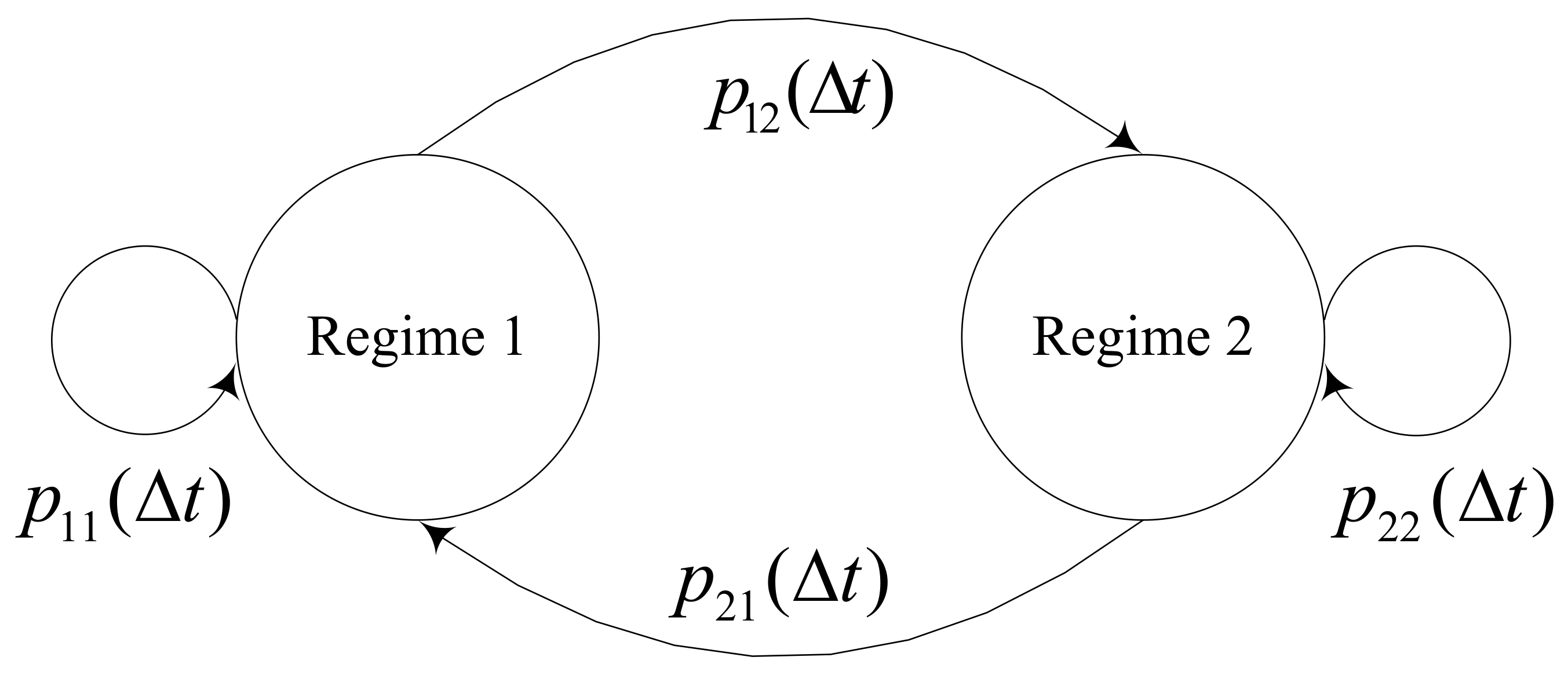
Column 7 shows the result of the valuation assuming that the R&D project starts in regime 1, and column 8 shows the result of it assuming that it starts in regime 2. The results in regime 2 of MRBL-MRS are greater than those in regime 1 across all projects. The differences range from $4.4 M to $28.0 M. This difference is due to the fact that the two regimes reflect different economic conditions. The difference of parameters between regime 1 and 2 resulted in the difference between Column 7 and Column 8. In our case study, the volatility of regime 2 is greater than that of regime 1. This difference had a critical influence on the difference in project values. From these results, it is revealed that MRBL-MRS captures risks caused by the uncertainty of the economic environment, which is represented by regime switching. This means that using the MRBL-MRS ROV model proposed in this paper, the decision maker can make different managerial decisions according to the current economic condition and expected changes in the future. Therefore, MRBL-MRS is a more flexible model than previous ROV models.

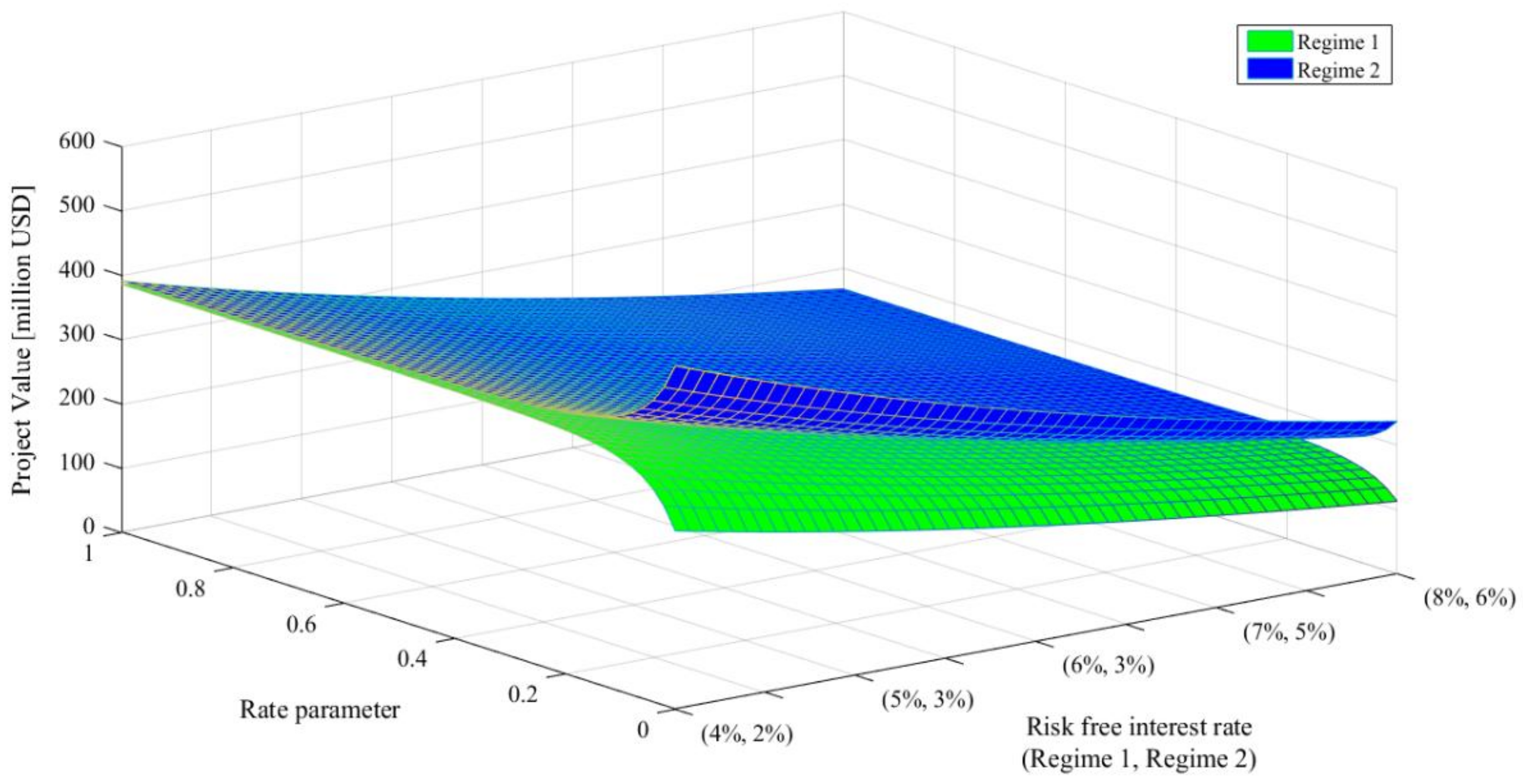
Further, we evaluated Project 1 with MRBL-MRS according to different values of the rate parameter and risk-free interest rate. The results are shown in

Table 5. Values of Project 1 with different rate parameters and risk-free interest rates.

λ	(r1 = 4%, r2 = 2%)		(r1 = 5%, r2 = 3%)		(r1 = 6%, r2 = 4%)		(r1 = 7%, r2 = 5%)
	Regime 1	Regime 2	Regime 1	Regime 2	Regime 1	Regime 2	Regime 1	Regime 2
0.00	277.4	534.2	224.0	437.7	179.7	357.9	143.1	291.9
0.05	339.6	459.5	275.6	375.7	222.8	306.3	179.0	248.9
0.10	363.7	429.1	295.8	350.3	239.7	285.1	193.2	231.1
0.15	374.5	414.7	304.9	338.3	247.3	275.0	199.6	222.7
0.20	379.7	407.1	309.3	331.9	250.9	269.7	202.7	218.2
0.25	382.5	402.7	311.5	328.3	252.9	266.7	204.2	215.7
0.30	384.0	400.0	312.8	326.0	253.9	264.8	205.1	214.1
0.40	385.4	396.9	313.9	323.4	254.9	262.6	205.9	212.3
0.50	385.9	395.1	314.4	322.0	255.2	261.4	206.2	211.3
1.00	386.4	391.4	314.8	318.9	255.5	258.9	206.4	209.1

and Figure 5. Rate parameter determines the probability of transition between regime 1 and regime 2. Rate parameter takes a value between 0 and 1. If it is close to 1, the transition probability is high, that is, the economic environment is likely to change. On the other hand, if the parameter value is close to 0, it means that the possibility of changing the economic environment is lowered. A risk-free interest rate affects the ROV as a risk-free discount rate. Thus, higher interest rates have an effect of lowering the resulting value. We varied rate parameter from 0.00 to 1.00 and risk-free interest rates for regimes 1 and 2 from ($r_1$ = 4%, $r_2$ = 2%) to ($r_1$ = 7%, $r_2$ = 5%). Other parameter values remain unchanged. Columns 2, 4, 6, and 8 of Table 5 present the project values in regime 1 for different speed of reversion values and columns 3, 5, 7, and 9 present those in regime 2. As the risk-free interest rate increases, the project value decreases and the value difference between regimes 1 and 2 also decreases. This is because as risk-free interest rate grows, the effect of discounting increases. Low 3 to 11 gives the project values for different values of rate parameters. As the rate parameter grows bigger, the transition probability from regime 1 to regime 2 increases. Thus, the project values in regime 1 increase, but those in regime 2 decrease. That is, when the rate parameter increases, the project values in regimes 1 and 2 converge. This means that the effect of regime switching by the Markov process is low for low values of the rate parameter, and it gradually increases as the rate parameter increases. You can see this characteristic in Figure 5. Therefore, when the transition probabilities between regimes are high, it is not important to the valuation result in which regime the project development starts. However, when the transition probability is low, it significantly affects the valuation results. Thus, management can decide to invest or wait, considering the current regime condition and the transition probability.

5. Conclusions

Effective management of the R&D portfolio is critical for a company’s R&D productivity, innovation, and financial performance, and furthers the firm’s sustainability or survival. An accurate valuation of R&D projects is an essential step towards R&D portfolio management. A real options approach for the valuation of R&D projects has an advantage to deal with various risks, and contributes to a firm’s strategic decision making for sustainable management. Therefore, ROV models have been considered an essential valuation method for decision making in R&D projects. However, current ROV models do not simultaneously adopt mean-reverting stochastic process and time-varying parameters. Therefore, this study proposed a valuation method with the mean-reverting binomial lattice model under Markov regime switching which can consider the market risks by applying time-varying parameters, such as volatility and risk-free interest rates.

We focused on the effective and sustainable management of the R&D portfolio in a pharmaceutical company, which is required risk management in the R&D stage, due to the long R&D period and huge R&D expenditure [23]. In this study, five clinical development projects of pharmaceutical companies were evaluated with the suggested model and compared with the valuation results of conventional DCF and other ROV models. The MRBL-MRS model suggested in this study represented more effective values than DCF, but corrected overestimated values by GBM. In addition, the results revealed that MRBL-MRS is an applicable and more flexible model that reflects changes of economic environment with a reflection of switching economic regimes compared to models that do not consider regime changing. Therefore, in practice, the method on the valuation of R&D projects proposed in this study can assist project managers of pharmaceutical companies in making effective decision making in R&D projects.

R&D project managers in pharmaceutical companies often face the difficulty of selecting an appropriate portfolio of R&D projects. The MRBL-MRS model suggested in this study captured risks caused by the uncertainty of the economic environment. In other words, it means that the MRBL-MRS model can provide more accurate information for decision making on portfolio selection for pharmaceutical R&D project managers by adapting mean reverting process and time-varying parameters resulting from changes of economic environment. Therefore, they can make different managerial decision according to the current economic condition and expected changes in the future.

Despite these contributions, this study has several limitations and future research is suggested. First, this study obtained the volatility, speed of sales reversion, and long-term mean of peak sales of a drug using Arca Pharmaceutical Index data, but the index does not fully represent the peak sales of a drug. Thus, future research is required to obtain a more accurate estimation of the parameters by using actual drug sales data or other complementary data. Second, this study only considered an option to abandon the project. Therefore, future research should consider other options in the real world for pharmaceutical R&D project valuation. In particular, the open innovation strategy by license agreements between small biotechnology firms and large pharmaceutical companies has become a popular business model in the pharmaceutical industry. Thus, licensing out or in options in pharmaceutical R&D project management should be considered in a future model. Third, this study employed a simple mean-reverting process. It was limited due to the fact that it did not describe exogeneous shocks despite providing a more realistic R&D project value than GBM. Therefore, future study should consider alternative stochastic processes, such as a mean-reverting jump diffusion process, for economic and technical exogeneous shocks during R&D periods.

References

1. Nigro, G.L.; Enea, G.; Morreale, A. A user friendly real option based model to optimize pharmaceutical R&D portfolio. J. Appl. Oper. Res. 2013, 5, 83–95. [Google Scholar]
2. Mikkola, J.H. Portfolio management of R&D projects: Implications for innovation management. Technovation 2001, 21, 423–435. [Google Scholar]
3. Trigeorgis, L.; Reuer, J.J. Real options theory in strategic management. Strateg. Manag. J. 2017, 38, 42–63. [Google Scholar] [CrossRef]
4. Walker, A.; Turner, S.; Johnson, R. Pharma and biotech valuations: Divergent perspectives. Bus. Dev. Licens. J. 2015, 22, 10–13. [Google Scholar]
5. Driouchi, T.; Bennett, D.J. Real options in management and organizational strategy: A review of decision-making and performance implications. Int. J. Manag. Rev. 2012, 14, 39–62. [Google Scholar] [CrossRef]
6. Marques, R.C.; Berg, S. Risks, contracts, and private-sector participation in infrastructure. J. Constr. Eng. Manag. 2011, 137, 925–932. [Google Scholar] [CrossRef]
7. Hassan, R.; De Neufville, R.; McKinnon, D. Value-at-risk analysis for real options in complex engineered systems. In Proceedings of the 2005 IEEE International Conference on Systems, Man and Cybernetics, Waikoloa, HI, USA, 12 October 2005; IEEE: New York, NY, USA; pp. 3697–3704. [Google Scholar]
8. Villiger, R.; Bogdan, B. Valuing pharma R&D: The catch-22 of DCF. J. Appl. Corp. Financ. 2005, 17, 113–116. [Google Scholar]
9. Villiger, R.; Bogdan, B. Real options are neither complicated nor unrealistic. Drug Discov. Today 2004, 9, 552–553. [Google Scholar] [PubMed]
10. Kellogg, D.; Charnes, J.M. Real-options valuation for a biotechnology company. Financ. Anal. J. 2000, 56, 76–84. [Google Scholar] [CrossRef]
11. Bogdan, B.; Villiger, R. Valuation in Life Sciences: A Practical Guide, 3rd ed.; Springer: Berlin/Heidelberg, Gerany, 2010. [Google Scholar]
12. Hauschild, B.; Reimsbach, D. Modeling sequential R&D investments: A binomial compound option approach. Bus. Res. 2015, 8, 39–59. [Google Scholar]
13. Cassimon, D.; Engelen, P.J.; Thomassen, L.; Van Wouwe, M. The valuation of a NDA using a 6-fold compound option. Res. Policy 2004, 33, 41–51. [Google Scholar] [CrossRef]
14. Wang, J.; Hwang, W.L. A fuzzy set approach for R&D portfolio selection using a real options valuation model. Omega 2007, 35, 247–257. [Google Scholar]
15. Myers, S.C.; Howe, C.D. Life-Cycle Financial Model of Pharmaceutical R&D; Program on the Pharmaceutical Industry Working Paper; Massachusetts Institute of Technology: Cambridge, MA, USA, 1997. [Google Scholar]
16. Schwartz, E.S. Patents and R&D as Real Options. Econ. Notes 2004, 33, 23–54. [Google Scholar]
17. Willigers, B.J.A.; Hansen, T.L. Project valuation in the pharmaceutical industry: a comparison of least-squares Monte Carlo real option valuation and conventional approaches. R&D Manag. 2008, 38, 520–537. [Google Scholar]
18. Hahn, W.J.; Dyer, J.S. Discrete time modeling of mean-reverting stochastic processes for real option valuation. Eur. J. Oper. Res. 2008, 184, 534–548. [Google Scholar] [CrossRef]
19. Banerjee, A. Real option valuation of a pharmaceutical company. J. Decis. Mak. 2003, 28, 61–73. [Google Scholar]
20. Yuen, F.L.; Yang, H. Option pricing with regime switching by trinomial tree method. J. Comput. Appl. Math. 2010, 233, 1821–1833. [Google Scholar] [CrossRef] [Green Version]
21. Costabile, M.; Leccadito, A.; Massabó, I.; Russo, E. A reduced lattice model for option pricing under regime-switching. Rev. Quant. Financ. Account. 2014, 42, 667–690. [Google Scholar] [CrossRef]
22. Zhou, Z.; Ma, J. Second-order lattice Boltzmann methods for PDEs of Asian option pricing with regime switching. Comput. Math. Appl. 2016, 71, 1448–1463. [Google Scholar] [CrossRef]
23. DiMasi, J.A.; Feldman, L.; Seckler, A.; Wilson, A. Trends in risks associated with new drug development: Success rates for investigational drugs. Clin. Pharmacol. Ther. 2010, 87, 272–277. [Google Scholar] [CrossRef] [PubMed]
24. Ng, R. Drugs: From Discovery to Approval, 3rd ed.; John Wiley & Sons: Hoboken, NJ, USA, 2015. [Google Scholar]
25. Glover, K.J.; Hambusch, G. Leveraged investments and agency conflicts when cash flows are mean reverting. J. Econ. Dyn. Control 2016, 67, 1–21. [Google Scholar] [CrossRef]
26. Wong, K.P.; Yi, L. Irreversibility, mean reversion, and investment timing. Econ. Model. 2013, 30, 770–775. [Google Scholar] [CrossRef]
27. Shen, Y.; Fan, K.; Siu, T.K. Option valuation under a double regime-switching model. J. Futures Mark. 2014, 34, 451–478. [Google Scholar] [CrossRef]
28. Mun, J. Real Options Analysis: Tools and Techniques for Valuing Investments and Decisions, 2nd ed.; John Wiley & Sons: Hoboken, NJ, USA, 2006. [Google Scholar]
29. Northrup, J. The pharmaceutical sector. In The Business of Healthcare Innovation; Burns, L.R., Ed.; Cambridge University Press: Cambridge, MA, USA, 2005; pp. 27–102. [Google Scholar]
30. Jacob, W.F.; Kwak, Y.H. In search of innovative techniques to evaluate pharmaceutical R&D projects. Technovation 2003, 23, 291–296. [Google Scholar]
31. Chu, K.C.; Wong, K.P. Progressive taxation and corporate liquidation policies with mean-reverting earnings. Econ. Model. 2010, 27, 730–736. [Google Scholar] [CrossRef]
32. Schwartz, E.S. The Stochastic Behavior of Commodity Prices: Implications for Valuation and Hedging. J. Financ. 1997, 52, 922–973. [Google Scholar] [CrossRef]
33. Bastian-Pinto, C.; Brandão, L.; Hahn, W.J. Flexibility as a source of value in the production of alternative fuels: The ethanol case. Energy Econ. 2009, 31, 411–422. [Google Scholar] [CrossRef]
34. Dixit, A.; Pindyck, R. Investment under Uncertainty; Princeton University Press: Princeton, NJ, USA, 1994. [Google Scholar]
35. Nelson, D.B.; Ramaswamy, K. Simple binomial processes as diffusion approximations in financial models. Rev. Financ. Stud. 1990, 3, 393–430. [Google Scholar] [CrossRef]
36. Cox, J.C.; Rubinstein, M. Options Markets; Prentice-Hall: Englewood Cliffs, NJ, USA, 1985. [Google Scholar]
37. Haahtela, T.J. Recombining Trinomial Tree for Real Option Valuation with Changing Volatility. 2010. Available online: https://ssrn.com/abstract=1932411 (accessed on 15 May 2017).
38. Aingworth, D.D.; Das, S.R.; Motwani, R. A simple approach for pricing equity options with Markov switching state variables. Quant. Financ. 2006, 6, 95–105. [Google Scholar] [CrossRef]
39. MarketWatch. Available online: https://www.marketwatch.com/investing/index/drg (accessed on 22 June 2017).
40. Qureshi, Z.P.; Seoane-Vazquez, E.; Rodriguez-Monguio, R.; Stevenson, K.B.; Szeinbach, S.L. Market withdrawal of new molecular entities approved in the United States from 1980 to 2009. Pharmacoepidemiol. Drug Saf. 2011, 20, 772–777. [Google Scholar] [CrossRef] [PubMed]
41. DiMasi, J.A.; Hansen, R.W.; Grabowski, H.G. The price of innovation: new estimates of drug development costs. J. Health Econ. 2003, 22, 151–185. [Google Scholar] [CrossRef]
42. DiMasi, J.A.; Grabowski, H.G.; Vernon, J. R&D Costs and Returns by Therapeutic Category. Drug Inf. J. 2004, 38, 211–223. [Google Scholar]
Figure 1. Basic building block of a binomial lattice.
Sustainability 10 00993 g001
Figure 2. State diagram of a two-state Markov process.
Sustainability 10 00993 g002
Figure 3. Binomial lattice for log peak sales.
Sustainability 10 00993 g003
Figure 4. Standard sales curve of a drug [11].
Sustainability 10 00993 g004
Figure 5. Values of Project 1 with respect to rate parameter and risk-free interest rate.
Sustainability 10 00993 g005