Optimizing the Construction Job Site Vehicle Scheduling Problem

Abstract

Concrete is one of the most important, versatile, and widely used building materials worldwide. Thus, an optimized delivery schedule of ready-mixed concrete (RMC) is a critical issue that can reduce CO₂ emission from RMC delivery vehicles. RMC is the most popular form of concrete material supplied to construction projects. When delivering RMC to construction sites, optimizing the transportation can be complex since there are many alternatives in terms of route choice. The objective of this research was to optimize the travel operation of RMC delivery vehicles to ensure that they travel via the most economical routes. The researchers developed a dynamic simulation model to solve this vehicle scheduling problem (VSP), applied an ant colony optimization (ACO) algorithm as a mathematical model, and analyzed the results achieved by the basic and improved ACO methods; the goals were to reduce travel distance and improve the simulation’s performance. Ultimately, the researchers found that the improved ACO method provided a more optimized transportation solution with a higher level of efficiency.

1. Introduction

Concrete is one of the most important, versatile, and widely used building materials worldwide. In 2016, 4.2 billion tons of concrete was produced globally to meet vast international production needs [1]. RMC (ready-mixed concrete) is the most popular form of concrete material, especially for urban construction projects. Scheduling its dispatch is a critical part of reducing CO₂ emissions from RMC delivery vehicles.

The RMC industry requires that strict standards be observed in terms of the time that elapses between production and distribution; this requirement increases the difficulty of production and distribution planning. Such planning involves maximizing the efficiency of the production sequence, pumping equipment, and operation of the transportation vehicles. Even though the composition of RMC tends to vary due to structural requirements and construction methods employed, construction sites require continuity in the unloading and placement of RMC because the material cannot be stored on site as inventory. Therefore, in most construction projects, optimizing RMC transportation is one of the most complex issues related to working with concrete. This issue becomes even more critical as the size of the construction site increases and the usage becomes higher. Increasing the efficiency of RMC management through the optimization of RMC usage will help to reduce CO₂ emissions from RMC delivery vehicles in the construction industry.

The objective of this research was to optimize the travel operation of RMC delivery vehicles to ensure that they travel by the shortest possible routes. The hypothesis of the research involves reducing the travel distance and time, which would lead to economic and environmental benefits regardless of the construction methods chosen for the reinforced concrete structures. Concrete production firms have made tremendous efforts to reduce the total delivery distance in given project-specific circumstances in order to achieve greater economic benefits. Of the various solutions proposed, solving the vehicle scheduling problem (or vehicle routing problem, VSP or VRP, respectively) is the most widely used method. VSP has been recognized as a critical logistics challenge in the construction industry. It includes finding the minimum cost of material delivery operations by selecting optimal routes from a supply location (or dispatch center) to various construction locations, as well as the return routes to the dispatch center, all without exceeding each vehicle’s load capacity. Since cost is closely related to distance, concrete supply firms have tried to find the shortest distances available for vehicles to travel while still satisfying delivery time requirements. The researchers in the current work developed a dynamic simulation model to solve this VSP for concrete placement work, applied an ant colony optimization (ACO) algorithm, and analyzed the results achieved via the basic and improved ACO methods; the goal was to reduce travel distance and improve the simulation’s performance.

2. Literature Review

2.1. Overview of the Vehicle Scheduling Problem

Most models have assumed that the direction of a vehicle cannot be reversed once it has begun moving towards its destination point [2]. However, if the model was capable of redirecting a moving vehicle to meet a new schedule and changing its next destination to be nearer to the vehicle’s current position, the model could achieve additional savings. To apply this “change rule,” the most current vehicle position would need to be monitored and the changing information communicated to the vehicle driver [2].

Two of the main existing model types related to finding optimal solutions to the VSP are the static and dynamic models. Static models require that before a delivery operation is scheduled, all necessary information for the operation be fixed. This information includes onsite construction locations, vehicle load capacity, delivery time, and the distances between construction locations and RMC placement sites. This model is somewhat unrealistic because in real-life applications all information is subject to change.

Dynamic models respond to these changes. In Ref. [3], it was argued that by adding objective functions, dynamic models enhance the degree of freedom to make decisions. The authors of Ref. [4] highlighted that dynamic models are different from static models in terms of their objectives. The main objective of a static model is cost savings from various alternatives, while dynamic models focus on improving the service level and ultimately increasing revenue.

For example, material suppliers may set an acceptance rule for customer requests. In Ref. [5], a method was proposed in which suppliers would not have the obligation to serve all customer requests. Users could apply a stochastic distribution from the body of customer requests to refine the acceptance criteria. The authors of Ref. [6] developed a scenario-based approach by generating artificial clients. Acceptance of the client’s request was dependent upon the scenario being able to support that request. For example, suppliers could reject a delivery request from highly remote areas and accept other requests.

2.2. Exact vs. Heuristic Algorithms

Existing research attempting to solve the VSP is categorized into two groups of algorithms: exact and heuristic. The most well-established exact algorithms include methods using linear and dynamic programming [7]. In Ref. [8], a formulation and the restriction of the linear programming were discussed. While both algorithm groups are valid, the researchers in the current work focused on heuristic algorithms because they are more widely applied to the various problem-solving practices common in the construction industry. The objective of a heuristic algorithm is finding a “near-optimal” solution within a reasonable amount of time. A solution could, for instance, simply approximate the exact solution but still be valuable [8]. Notable heuristic algorithms for solving the VSP include the Clarke and Wright [9], sweep [10], tabu search [11], and ant colony [12,13] algorithms.

2.3. Ant Colony Optimization (ACO)

The ant colony optimization (ACO) algorithm was developed based on a computational model of real ants’ behavior [12]. By definition, ACO is a metaheuristic approach for deriving approximate solutions from real ants’ behavior in order to find the shortest path from one location (a food source) to a destination (the nest). It has been widely applied to various logistics optimization problems. The basic rule of ACO is that ants follow pheromone information when they have multiple routes from which to select, and they usually find the shortest route because more pheromone is deposited on the shorter path, based on a probability function [12]. As mentioned earlier, the researchers applied the ACO algorithm to solve the VSP.

2.4. Mathematical Model of ACO for Route Construction

The core algorithm for ACO that was applied in this research is discussed below. Initially, an individual ant is located at a random point. In each step of the simulation, ant k chooses a route according to a probabilistic choice function. Equation (1) shows the algorithm for ant k, located at point i; ant k chooses to go to point j at the tth iteration [14]:

$$p_{ij}^k=\frac{{[{\tau }_{ij}(t)]}^{\alpha }·{[n_{ij}]}^{\beta }}{{\displaystyle \sum }l\in N_i^k{[{\tau }_{il}(t)]}^{\alpha }·{[n_{il}]}^{\beta }}, \mathrm{if} j \in N_i^k ,$$

(1)

where η_ij represents an available heuristic value, α and β are two parameters for verifying the heuristic information and determining the relative influence of the pheromone on the trail [15], and $N_i^k$ represents the possible places ant k has not been located. In Ref. [14], the authors explained that “if α = 0, the closest points are more likely to be selected; this corresponds to a classical stochastic algorithm with multiple starting points since ants are randomly distributed on the locations. If β = 0, only pheromone amplification is at work; this method will lead to the rapid emergence of a stagnation situation with the corresponding generation of tours, which, in general, will lead to a situation in which all the ants follow the same path and construct the same solution.” This function leads to a trade-off between the influence of the heuristic information and the pheromone trails [14].

The pheromone trails become possible routes once all of the ants have traveled all the routes after the pheromone trails have been updated. The pheromone strength decreases along all routes by a constant factor to allow each ant to add pheromone to the routes it has visited [16]. This function is shown in Equation (2):

$${\mathsf{\tau }}_{ij}(t+1)=(1-\rho )·{\tau }_{ij}(t)+{\displaystyle \sum }_{k=1}^m\Delta {\tau }_{ij}^k(t)$$

(2)

where 0 < ρ ≤ 1 describes an evaporation function on the pheromone trail. The parameter ρ limits accumulation of the pheromone on the trails by eliminating longer routes that have previously been passed. If the ants do not choose a route, the pheromone accumulated on that route decreases exponentially [14]. The variable $\Delta {\mathsf{\tau }}_{ij}^k(t)$ is the amount of pheromone ant k deposits on the routes it has passed. Equation (3) represents the function:

$$\Delta {\mathsf{\tau }}_{ij}^k(t)= \{\begin{array}{c}\frac{1}{L^k(t)}, \mathrm{if} \mathrm{arc}(i,j) \mathrm{is} \mathrm{used} \mathrm{by} \mathrm{ant} k \\ 0, \mathrm{otherwise} \end{array}$$

(3)

where L^k(t) represents the length of the route the kth ant passed. According to this equation, “the better the ant’s tour is, the more pheromone is received by arcs belonging to the tour” [14]. In this algorithm, the shorter routes accumulate a greater quantity of pheromone because they have recorded more travel.

3. Modeling the RMC Vehicle Operation

This section is divided into subsections. It provides a concise and precise description of the experimental results, their interpretation, and the conclusions drawn.

3.1. Description of RMC Vehicle Operation

The RMC vehicle operation process involves five steps, which are illustrated in Figure 1: (1) RMC production; (2) loading at the dispatch center; (3) traveling to a construction site; (4) RMC placement at the construction location; and (5) returning to the dispatch center. When the vehicle arrives at the construction site, it must wait before placing the RMC at the construction location that requires concrete, as illustrated in Figure 2.

A dynamic model for the VSP was selected as the modeling method in this research because it is a developed form of static modeling that makes changes possible, as was described in the literature review. The dispatch center only controls certain information, and whatever information the center does not have is subject to change. This changeable information includes adjustments to the same construction locations. In practice, even after a delivery order has been given, known information may change during the delivery process. If the model were to take all possible conditions into consideration, the whole system would become very complex and uncontrollable and its deviation would increase with the multiple changing variables. Therefore, the researchers focused only on adding new construction locations by applying the dynamic model to the VSP.

3.2. Constituent Elements of the VSP

The constituent elements of the VSP include the construction site, vehicle, RMC, construction locations, constraints, and objective function.

1) Construction Site

The function of a construction site is to supply the physical environment for a vehicle to work. Once the vehicle loaded with RMC arrives at the site, it needs to wait to be called to work in a particular spot.

2) Vehicle

The vehicle is the transportation equipment used for RMC transportation. The essential attributes include the load capacity, number of vehicles available, load condition, and time limitations. We classified the vehicle by capacity, that is, the small and large vehicles cover up 6 m³ and 8 m³, respectively.

3) RMC Material

The essential attributes include type, weight, volume, production time, delivery time, and arrival time (i.e., arrival at the construction work site).

4) Construction Location

This refers to the specific location where the vehicles need to place the RMC.

5) Constraints

A vehicle must meet basic conditions such as being fully or not fully loaded and soft-time vs. hard-time window. Also, the conditions need to include vehicle operators’ performance (productivity), time delay by site congestion, disruption by vehicle breakdown, and so on.

6) Objective Function

An objective function can include more than one condition. For this research, four functions were applied:

a)

Shortest route and time: a vehicle travels to all of the construction locations via the shortest distance and the entire transport process incurs the shortest time.

b)

Lowest cost and least number of vehicles: the entire transportation process incurs the lowest cost and the entire transportation process uses the least number of vehicles to accomplish the goal.

3.3. Design of the Experiment

The underlying process for the experimental VSP model involved delivering the RMC to a range of delivery points with each delivery point having time requirements. The goal was to determine an appropriate delivery vehicle driving route from the dispatch center through all delivery points and ultimately returning to the dispatch center while achieving the minimum total transportation cost. The researchers considered the cost savings provided by two types of vehicles, first using a larger vehicle to determine the optimal path and then (after determining the optimal path), if the total load capacity of all of the larger vehicles was less than that of a smaller vehicle, the smaller vehicle making the delivery instead of the larger vehicle. This required reasonable arrangements for the vehicles’ driving route and minimizing the total transportation costs while meeting the following conditions [17]:

The following conditions from 1 to 4 were applied to the first object function (shortest route and time) and the fifth condition to the second function (lowest cost and least vehicle number).

1)

All vehicles leaving from the dispatch center had to return to the dispatch center after completing the delivery task.

2)

The construction point demand on each distribution route could not exceed the vehicle’s full load capacity.

3)

The total distance of each distribution route could not exceed the vehicle’s maximum travel distance.

4)

The time window for each demand point had to be met and the total operation time of the vehicle could not exceed the maximum work time.

5)

The specific delivery point, delivery volume, and cost with the fastest speed from the dispatch center to the delivery point had to be known to the dispatch center before the schedule was made.

Equation (4) shows the objective functions.

As seen in Equation (4), the objective function f and the transportation routes, vehicle cost, and transportation volume are all related. The variable I_ijk is the shortest distance in the network, q_ijk is vehicle k’s transportation volume from point i to point j, and p_i is the transportation cost per unit weight from the dispatch center to point i. Equation (4) is as follows:

$$\mathrm{f}=\min {\displaystyle \sum }_{k=1}^K{\displaystyle \sum }_{i=0}^N{\displaystyle \sum }_{i\ne j}^N{I}_{ij}{x}_{ijk}{q}_{ijk}{p}_i$$

(4)

where the larger vehicle’s deadweight is Q_b, the smaller vehicle’s deadweight is Q_s (see Equation (5)), and two types of vehicles’ maximum travel distances are both D (see Equation (6)). For example, if a vehicle is required to travel to three delivery points, the demand for each delivery point is q_i (i = 1, 2, 3). Equation (5) ensures that the total demand of each point on the path does not exceed the vehicle’s load capacity. Equation (6) ensures that the total length of each delivery path does not exceed the vehicle’s maximum travel distance. Equations (5) and (6) are as follows:

$${\displaystyle \sum }{q}_{r_{ki}}\le Q,$$

(5)

$${{\displaystyle \sum }}_{i=1}^{R_k}{d}_{r_{k(i-1)r_{ki}}}+d_{r_{nk}{r}_{k0}}\sin (n_k)\le D.$$

(6)

Equations (7) and (8) ensure that the vehicle’s total work time does not exceed the maximum total working hours, and Equation (9) shows that the demand points on each path have to obtain distribution services. In Equation (9), n_k represents vehicle k’s demand distribution points. In Equation (8), R_k indicates the travel path of vehicle k and t_rki shows the moment when the vehicle k reaches point i. In Equation (7), w_rki signifies vehicle k’s time cost for accomplishing the task. Equations (7) and (8) ensure that the total work time does not exceed the maximum total working hours. Equation (9) indicates the demand points on each path that have to obtain distribution services. Equations (7)–(9) are as follows:

$$\max (t_{r_{ki}}+{\mathrm{w}}_{r_{ki}}+{\mathrm{t}}_{r_{kj{r}_{ko}}})\le {\mathrm{LT}}_0$$

(7)

$$\min (t_{r_{ki}}-t_{r_{ki}{r}_{k0}})\ge {\mathrm{ET}}_0$$

(8)

$${\displaystyle \sum }_{k=1}^c{n}_k=L$$

(9)

In Equation (10), the time window [ET_i, LT_i] represents task i’s earliest and latest start times, and v denotes the average speed of each vehicle. Equation (10) specifies that if the time cost initially fits the time window, the user could take s_i = t_0i. If t_0i < ETi, the user takes s_i = ET_i (which means that if the vehicle was earlier than ET_i, it should stay at point i); otherwise, the user takes t_ij = d_ij/v.

$$E{T}_i\le t_{0i}\le L{T}_i$$

(10)

In Equation (11), s_i represents the vehicles’ moment of arrival at delivery point i and t_ij signifies the time required to travel from delivery point i to delivery point j. The variable T_i indicates the unloading time; if the vehicle arrives earlier than ET_i, it has to wait at i. The variable LT_i indicates the latest arrival time. If the vehicle arrives later than the time of arrival, task i needs to be rescheduled so that a smaller vehicle would deliver on time.

$$s_j=s_i+T_i+t_{ij}$$

(11)

$${\displaystyle \sum }_{i=1}^{m_k}{C}_{r_{ki}}\le D_s$$

(12)

Equation (11) shows that if the time cost of the vehicle arriving at the next delivery point is j, ET_j ≤ s_j ≤ LT_j. Equation (12) represents that vehicle k completed the task with little weight and less than the smaller vehicle’s load capacity; the user could thus employ the smaller vehicle instead of the larger one in order to save costs.

An initial model was built using a static model. A sample construction site was developed with eight construction locations requiring RMC, as shown in Figure 3. All vehicles left from the dispatch center fully loaded and the maximum capacity was eight tons. The average speed of each vehicle was 60 km/h for the x-coordinate and 80 km/h for the y-coordinate. The coordinates of the dispatch center were [0,0], and the vehicles’ departure times were marked 0.

Table 1. Input variables for the initial model.

Spot Number	Download Concrete Weight (ton)	Time Window	Spot Coordinates	Spot Number	Downloaded Concrete Weight (ton)	Time Window	Spot Coordinates
1	1.5	[2, 6]	(20, 85)	7	2.5	[1.5, 8]	(120, −15)
2	1.7	[1, 8]	(70, 40)	8	2.6	[1.5, 6]	(90, −20)
3	2.2	[0, 7]	(−10, 150)	A	1.5	[1, 4]	(30, 70)
4	1.5	[2.5, 7]	(−20, 60)	B	1.3	[2, 6.5]	(−50, 100)
5	1.3	[1.5, 6]	(−45, −90)	C	2	[2.5, 7]	(−30, −70)
6	2.1	[2, 6]	(−70, −50)	D	1.7	[3, 8]	(60, −50)

shows all other input data for the initial model.

The initial static model represented in Figure 3 indicated that the task required three vehicles, and the routes consisted of route 1: 0-1-3-4-0, route 2: 0-2-7-8-0, and route 3: 0-5-6-0 based on their geographical proximity. Then, the same site required four new construction locations—namely, A, B, C, and D—for the delivery procedure. The placement of the four new locations is indicated in Table 1. First, the user specified to the dispatch center that a new construction location “A” was required. In order to reschedule the new route, the dispatch center made the vehicle driver change route to accommodate the new schedule, in that the vehicle located in closest proximity to location A had to go to location A and then resume the original route to accomplish the task, as seen in Figure 4.

Next, the vehicle proceeded onward. The dispatch center then received new information that a new location “B” had been added. The dispatch center rescheduled the route, as shown in Figure 5. The vehicle on the first route was directed to the new location B due to its proximity. Routes two and three remained unchanged.

After some time, the dispatch center received information that a new construction location “C” had been added near spot 6. After finishing spot 5, the vehicle traveling route 2 had to travel to location C before returning to the dispatch center. Figure 6 shows the new location C route diagram.

The result, however, was that the amount of concrete required exceeded the vehicle’s load capacity on routes 1 and 2. After a while, a new location “D” was added but the vehicle on route 2 was not carrying enough material. Thus, the vehicles on routes 2 and 3 would need to travel simultaneously to spot D, according to the requirements for concrete (see Figure 7).

In short, when new construction locations are added, the user must convert the static model into a dynamic model. To accomplish this conversion, the user must confirm the information already known via the static model and make new arrangements as the original route progresses. ACO helps to formulate the best route arrangement to solve the problems related to the addition of new locations. To produce the experiment’s model, the researchers selected 15 delivery points and a dispatch center and scheduled the optimal path. The parameters were set as shown in

Table 2. Simulation parameter settings.

Alpha (Important Factors)	Beta (Visibility Coefficient)	NC_Max (The Maximum Number of Iterations)	Q (Information Update Parameters)	W (Smaller Car Deadweight)
1	5	50	8	6

. The model was then simulated on the MATLAB platform.

4. Simulation Results

4.1. Results from the Basic ACO Model

To illustrate the effectiveness of the ACO model, the researchers compared the basic and improved ant colony algorithms for the VSP. Both algorithms responded to realistic route conditions. Ideal road conditions do not respond to realistic interference factors in that vehicle speed is kept constant and does not consider traffic jams, damage to the road or vehicles, or other incidents that might occur during transportation. The developed models incorporated specific real traffic information as follows:

a)

Daily traffic jam during rush hour from 7:00 to 9:00 a.m. and from 5:00 to 7:00 p.m.

b)

The road route between two delivery points could not always be a straight line.

c)

The vehicle ran at a different speed if driven on a different type of road. Theoretical input for the delivery location, time windows, and delivery amounts are shown in

Table 3. Delivery information.

Delivery Point Coordinates	Time Window	Delivery Amount (ton)	Delivery Point Coordinates	Time Window	Delivery Amount (ton)	Delivery Point Coordinates	Time Window	Delivery Amount (ton)
(20, 85)	[2, 6]	1.5	(10, 150)	[0, 7]	1.5	(−70, −50)	[2, 6]	1.6
(70, 40)	[1, 8]	1.7	(−20, 60)	[2.5 ,7]	1.4	(30, −70)	[3, 9]	2.7
(15, 100)	[2, 9]	1.5	(100, −10)	[2, 10]	2.2	(120, −15)	[1.5, 6]	2.5
(60, 20)	[4, 7]	3	(−40, −60)	[3, 8]	1.3	(90, −20)	[1.5, 8]	2.6
(100, 10)	[2.5, 8]	2.2	(−45, −90)	[1.5, 6]	2.1	(50, −105)	[3, 10]	2.1

. The coordinates unit for the delivery point was kilometers, time window unit was hours, delivery volume unit was tons, and coordinates of the dispatch center were [0,0].

The simulation results from the basic ACO model for the VSP under real road conditions are shown in Figure 8. Four routes were chosen as the optimal solution to the VSP, with the best length (i.e., the shortest distance) of 1530 kilometers.

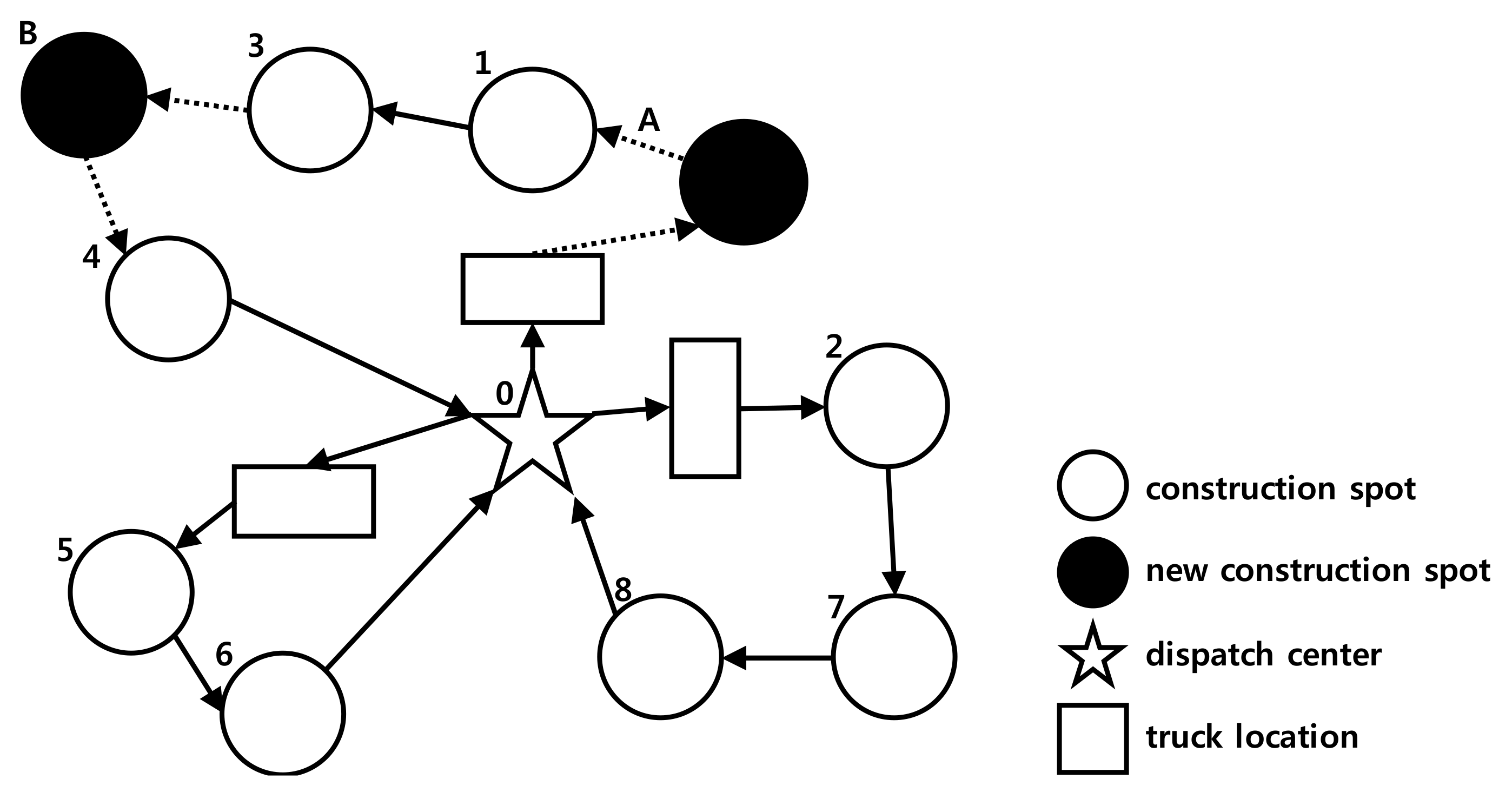
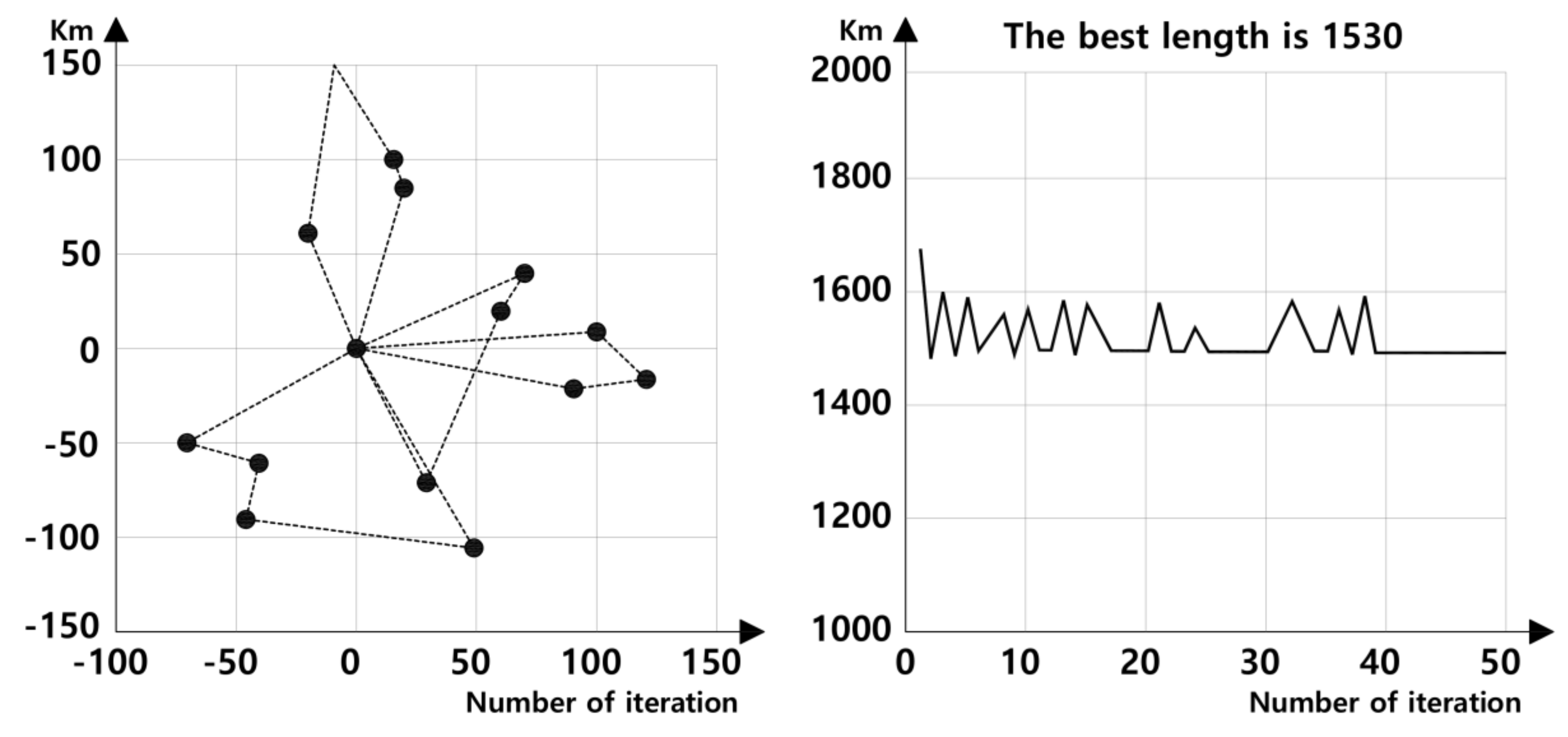
4.2. Results from the Improved ACO Model

The simulation task using the basic ACO model took a longer distance and time because each individual ant colony movement was random. With a larger ant population, it was difficult to determine the optimal solution in a short period of time. The researchers focused on improving two aspects of the basic ant colony algorithm. The improvement measures were as follows.

4.2.1. Volatility Factor Change from Constant to Variable Function

In the basic ACO model, the volatility factor was fixed even though in real life the pheromone concentration increases with an increase in the volatility factor. It decreases when the volatility factor decreases. In this case, a constant factor becomes a variable function, as shown in Equation (13):

$${\mathsf{\tau }}_{ij}(t+1)=(1-\rho ){\mathsf{\tau }}_{ij}(t)+{\rho }_1\Delta {\mathsf{\tau }}_{ij}(t)$$

(13)

The equation shows the pheromone density on path ij at moment (t + 1). Concentration on Δτ_ij(t) is a pheromone increment and the volatility factor is $\rho$.

4.2.2. Introduction of the “Incentive” Mechanism

At the end of the basic ACO model’s iteration, the simulation results from each path showed high variability. Because the basic ACO model only incorporated positive ACO feedback, no matter how good the search solutions were, the pheromones on every path tended to increase to a certain extent. For this reason, the researchers incorporated an “incentive” mechanism to reward the best and punish the worst paths.

After the ants went through all the tasks once, if the path showed a better result than the previous optimal path, the pheromones increased on the latter path in the improved ACO model. Otherwise, the pheromones on the latter path were reduced. The introduction of an incentive mechanism for pheromone control is shown in Equation (14):

$$\Delta {\mathsf{\tau }}_{ij}(t)=\sigma \frac{L_c(t+1)-L_b(t)}{L_b(t)+L_c(t+1)}$$

(14)

where σ is a reference factor, L_b(t) is the optimal solution path, and L_c(t + 1) is the present path. If the current path was better than the historical optimal path (Δτ_ij(t) > 0), a certain amount of pheromone reward was given. Conversely, if the current path was not an optimal path as compared to the historical optimal path (Δτ_ij(t) < 0), a certain amount of pheromone was decreased as punishment. The system diagram with the improved ACO model is shown in Figure 9.

After the experiment, it was determined that the improved ACO model achieved optimum vehicle scheduling, as shown in Figure 10. The improved ACO model applied to the VSP conclusively achieved better results and an improved level of efficiency.

While the number of vehicles in Figure 9 and Figure 10 was the same, the results obtained using the improved ACO model were better because there was a saving in operating costs (i.e., a shorter distance was traveled) to a small extent (1530 vs. 1440). In addition, the improved ACO model achieved a better relationship between the line length and number of iterations, indicating that it reached the optimal solution in a shorter simulation time. This result showed ACO as an effective modeling method to find the optimum solution for traveling problems, especially if dynamic and heuristic functions were utilized. Also, the improved function was a valid method to make the simulation more efficient.

5. Conclusions

Planning RMC delivery vehicles’ travel operations require selection of the optimal or near-optimal solution to maximize economic benefits. The shortest route to increase the efficiency of RMC management leads to the most economical and environmentally-friendly choice by consuming the minimal amount of fuel and reducing CO₂ emissions. Previous studies have solved the VSP by using various algorithms and proving the possible solutions. The researchers developed a theoretical model for the RMC delivery operation based on a dynamic modeling method, in order to improve practicality by responding to changing information during the operation. Then, the researchers developed an algorithm for the model from one basic and one improved ACO, with the goal of achieving better results and a higher simulation efficiency. The improved ACO model applied a variable volatile function and introduced an incentive mechanism. In conclusion, the ACO-based model provided an efficient heuristic method to solve the VSP for the delivery of RMC in the construction industry. By using the developed model, project-specific information can be input to more accurately and efficiently simulate the RMC delivery task. The limitation of this research is that even though the model was capable of accommodating new construction locations during operation, the practicality of the model could still be improved by applying the model to real-life practice. The researchers will continue to apply the ACO-based model to test more optimized RMC delivery routes and enhance the suggested methodology, as well as collect measured data from real-world projects to validate the developed model.

References

1. U.S. and World Cement Production 2017. Statistic. Available online: https://www.statista.com/statistics/219343/cement-production-worldwide (accessed on 30 April 2018).
2. Ichoua, S.; Gendreau, M.; Potvin, J.-Y. Diversion issues in real-time vehicle dispatching. Transp. Sci. 2000, 34, 426–438. [Google Scholar] [CrossRef]
3. Pillac, V.; Gu´eret, C.; Medaglia, A. Dynamic Vehicle Routing Problems: State of the Art and Prospects; Technical Report 10/4/AUTO; Ecole des Mines de Nantes: Nantes, France, 2011. [Google Scholar]
4. Psaraftis, H.N. Dynamic vehicle routing: Status and prospects. Ann. Oper. Res. 1995, 61, 143–164. [Google Scholar] [CrossRef]
5. Gendreau, M.; Guertin, F.; Potvin, J.-Y.; Taillard, E. Parallel tabu search for real-time vehicle routing and dispatching. Transp. Sci. 1999, 33, 381–390. [Google Scholar] [CrossRef]
6. Hvattum, L.M.; Lokketangen, A.; Laporte, G. Solving a dynamic and stochastic vehicle routing problem with a sample scenario hedging heuristic. Transp. Sci. 2006, 40, 421–438. [Google Scholar] [CrossRef]
7. Laporte, G.; Louveaux, F.; van Hamme, L. An integer l-shaped algorithm for the capacitated vehicle routing problem with stochastic demands. Oper. Res. 2002, 50, 415–423. [Google Scholar] [CrossRef]
8. Haupt, R.L.; Haupt, S.E. Practical Genetic Algorithms; John Wiley & Sons: Hoboken, NJ, USA, 2004. [Google Scholar]
9. Clarke, G.; Wright, J.W. Scheduling of Vehicles from a Central Depot to a Number of Delivery Points. Oper. Res. 1964, 2, 568–581. [Google Scholar] [CrossRef]
10. Wren, A.; Holliday, A. Computer scheduling of vehicles from one or more depots to a number of delivery points. Oper. Res. Q. 1972, 23, 333–344. [Google Scholar] [CrossRef]
11. Gendreau, M.; Hertz, A.; Laporte, G. A Tabu Search Heuristic for the Vehicle Routing Problem. Manag. Sci. 1994, 40, 1276–1290. [Google Scholar] [CrossRef]
12. Dorigo, M.; Gambardella, L.M. Ant Colony System: A Cooperative Learning Approach to the Traveling Salesman Problem. IEEE Trans. Evol. Comput. 1997, 1, 53–66. [Google Scholar] [CrossRef]
13. Dorigo, M.; Di Caro, G.; Gambardella, L.M. Ant Algorithms for Discrete Optimization; Artificial Life, MIT Press: Cambridge, MA, USA, 1999. [Google Scholar]
14. Dorigo, M.; Gambardella, L.M. Ant colonies for the travelling salesman problem. Biosystems 1997, 43, 73–81. [Google Scholar] [CrossRef]
15. Qi, C. An Ant Colony System Hybridized with Randomized Algorithm for TSP. In Proceedings of the Eighth ACIS International Conference on Software Engineering, Artificial Intelligence, Networking, and Parallel/Distributed Computing, Qingdao, China, 30 July–1 August 2007; pp. 461–465. [Google Scholar]
16. Stützle, T.; Marco, D. ACO algorithms for the traveling salesman problem. In Evolutionary Algorithms in Engineering and Computer Science; John Wiley & Sons: Hoboken, NJ, USA, 1999; pp. 163–183. [Google Scholar]
17. Wei, M.; Bin, Y. Research on optimization of vehicle routing based on Hopfield neural network. In Proceedings of the 2011 IEEE 2nd International Conference on Software Engineering and Service Science (ICSESS), Beijing, China, 15–17 July 2011; pp. 157–159. [Google Scholar]
Figure 1. Ready-mixed concrete (RMC) vehicle operation process.
Sustainability 10 01381 g001
Figure 2. RMC vehicle process for placement.
Sustainability 10 01381 g002
Figure 3. Initial static model for the vehicle scheduling problem (VSP). The dispatch center indicates the RMC production center in Figure 1.
Sustainability 10 01381 g003
Figure 4. Model for the addition of a new location A.
Sustainability 10 01381 g004
Figure 5. Model for the addition of a new location B.
Sustainability 10 01381 g005
Figure 6. Model for the addition of a new location C.
Sustainability 10 01381 g006
Figure 7. Model for the addition of a new location D.
Sustainability 10 01381 g007
Figure 8. Results from the basic ant colony optimization (ACO) model.
Sustainability 10 01381 g008
Figure 9. System diagram for the improved ACO.
Sustainability 10 01381 g009
Figure 10. Results from the improved ACO model.
Sustainability 10 01381 g010