The Causal Effects of Trade and Technology Transfer on Human Capital and Economic Growth in the United Arab Emirates

Abstract

This research empirically investigates the causality between trade, technology, human capital and economic growth in the United Arab Emirates (UAE) over the period 1980–2016. To investigate the existence of a long-run relationship between the variables, this study performs the Johansen cointegration test, while the direction of the short-run causality is examined by applying the Granger causality test in a Vector Error Correction Model (VECM) framework. Moreover, a modified Wald test in an augmented Vector Autoregressive Model is applied in order to find the direction of the long-run causality. This research provides evidence to support a short-run bi-directional causality between primary imports and economic growth, while an indirect causality runs from manufactured imports and human capital to economic growth, through exports and primary imports. Empirical results do not provide evidence of either an Import-Led growth (ILG) or Export-Led Growth (ELG) hypothesis in the long-run, while no causality runs from primary imports, manufactured imports or exports to human capital.

1. Introduction

A number of previous studies indicate that imports are a major channel for technology transfer and knowledge diffusion, which are essential to improving productivity and economic growth [1,2,3,4]. In return, economic growth can cause an expansion of exports, especially of manufactures, which can offer knowledge spillovers and other externalities, creating virtuous circles of cumulative causation. In particular, further economic growth creates new needs, which cannot be covered by the domestic production, leading to a further increase in the level of imports, especially in imports of capital equipment [5,6,7]. In general, “rapid export growth facilitates the acquisition of capital goods and technology transfer that drives economic growth, and rapid growth provides the means to finance investment in physical and human capital that supports more rapid export growth” [8] (p. 6).

This research will empirically investigate the causality between new technologies (embodied in manufactured imports), exports, human capital and economic growth in the UAE, which is the most diversified economy in the Gulf Cooperation Council (GCC) region.

The UAE has achieved strong economic growth and significant export diversification over the last three decades. In 2016, the Gross Domestic Product (GDP) of UAE increased eight times, compared to the 1980 level, with an average growth per annum of 6.5 percent. Eight years after the global financial crisis of 2008/09, the UAE GDP has increased by 10.5 percent, with an annual average growth rate of approximately 4.3 percent, when the global average growth rate for the same period is estimated at around 2.3 percent.

In 2016 the UAE was ranked 19th among the leading exporters and importers in world merchandise trade [9]. In particular, the value of UAE merchandise exports in 1980 is estimated at around US$21.97 billion, rising to US$266 billion in 2016, with an average growth per annum of 9%. During the same period, the UAE have experienced significant export diversification, which is reflected by the share of manufactured exports in merchandise exports. In particular, the share of manufactured exports in total merchandise exports increased from around 3% in 1980 to approximately 27% in 2016.

The value of UAE merchandise imports in 1980 was estimated at US$10.22 billion, rising to US$353.8 billion in 2016, with an average growth per annum of 11.1%. The share of manufactured imports in total merchandise imports decreased from around 68.8% in 1980 to approximately 58.3% in 2016, indicating a decreasing demand for high technological imports.

In the last three decades, the working age population of UAE has increased from approximately 735.5 thousand in 1980 to 7.9 million in 2016, an increase of about 10 times. In 1990 the non-national population was estimated at around 1.30 million, representing 70.2 percent of the total UAE population. In 2000, the non-national population reached approximately 2.44 million, while in 2015 it reached 8.1 million, representing 77.5 and 88.4 of the total population respectively [10].

Accordingly, this research attempts to investigate whether new technologies (embodied in manufactured imports) cause further export expansion, which in return could accelerate human capital accumulation and economic growth in the UAE in the short-run or long-run. In sum, this study will help in designing future policies for enhancing and sustaining economic growth in UAE.

2. Literature Review

Most of the previous studies examine the effects of exports on economic growth, while fewer studies focus on imports, as imports are considered to be a leakage of export revenues, which lead to a lower rate of growth. In the case of the Export-Led growth hypothesis (ELG), export growth increases the inflows of investment in those sectors where the country has comparative advantage and this could lead to the adoption of advanced technologies, improving human capital accumulation [11,12] and increasing the rate of economic growth [13,14,15,16,17,18,19,20]. In addition, the increase in the inflows of foreign exchange improves the country’s capacity to import technologically advanced capital goods, which are essential to improving productivity and economic growth [6,21,22]. Therefore, in the ELG hypothesis, exports positively affect national income through imports.

In the case of the Imports-Led Growth (ILG), an increase in imports, especially in consumer goods, encourages domestic-substituting firms to innovate in order to be more competitive, expanding their investments in new technology and improving productivity [11,23]. In parallel, an increase in imported goods can cause an increase in export-oriented production, as some categories of imports are used as inputs for merchandise exports and especially for manufactured exports, which are beneficial for human capital. Therefore, imports positively affect economic growth through technology and expansion of manufactured exports, as this category of exports offers knowledge spillover effects and positive externalities to non-export sectors, leading to further economic growth [24,25].

In both ELG and ILG, an increase in exports and imports respectively, lead to human capital accumulation, through the adoption of advanced technologies, while in return human capital positively contributes to the efficient use of adopted technology, leading to economic growth. In the ELG, the adoption of advanced technology takes place due to the increase in inflows of foreign exchange, which allow the expansion of imports, while in the case of ILG, the adoption takes places through R&D investments and innovation efforts to compete with foreign markets. Therefore, previous studies mentioned above indicate that trade, technology, human capital and economic growth are interrelated, but in the case of an oil producing country like UAE, what is the direction of the causality?

Most of the empirical studies have used bivariate or trivariate models in order to test the validity of the ELG and ILG hypotheses and this might lead to misleading and biased results. In other words, these studies have examined the relationship between exports, imports and economic growth, ignoring the complex causal nature of events and the human dimension of economic growth. For this reason, the present study includes variables omitted in most of the previous studies, such as human capital and physical capital.

The remaining sections of this paper are organized as follows; Section 3 describes the data sources, chosen methodology and empirical models. Section 4 reports and interprets the empirical results, while Section 5 presents the summary and conclusion of this research.

3. Data and Methodology

3.1. Data

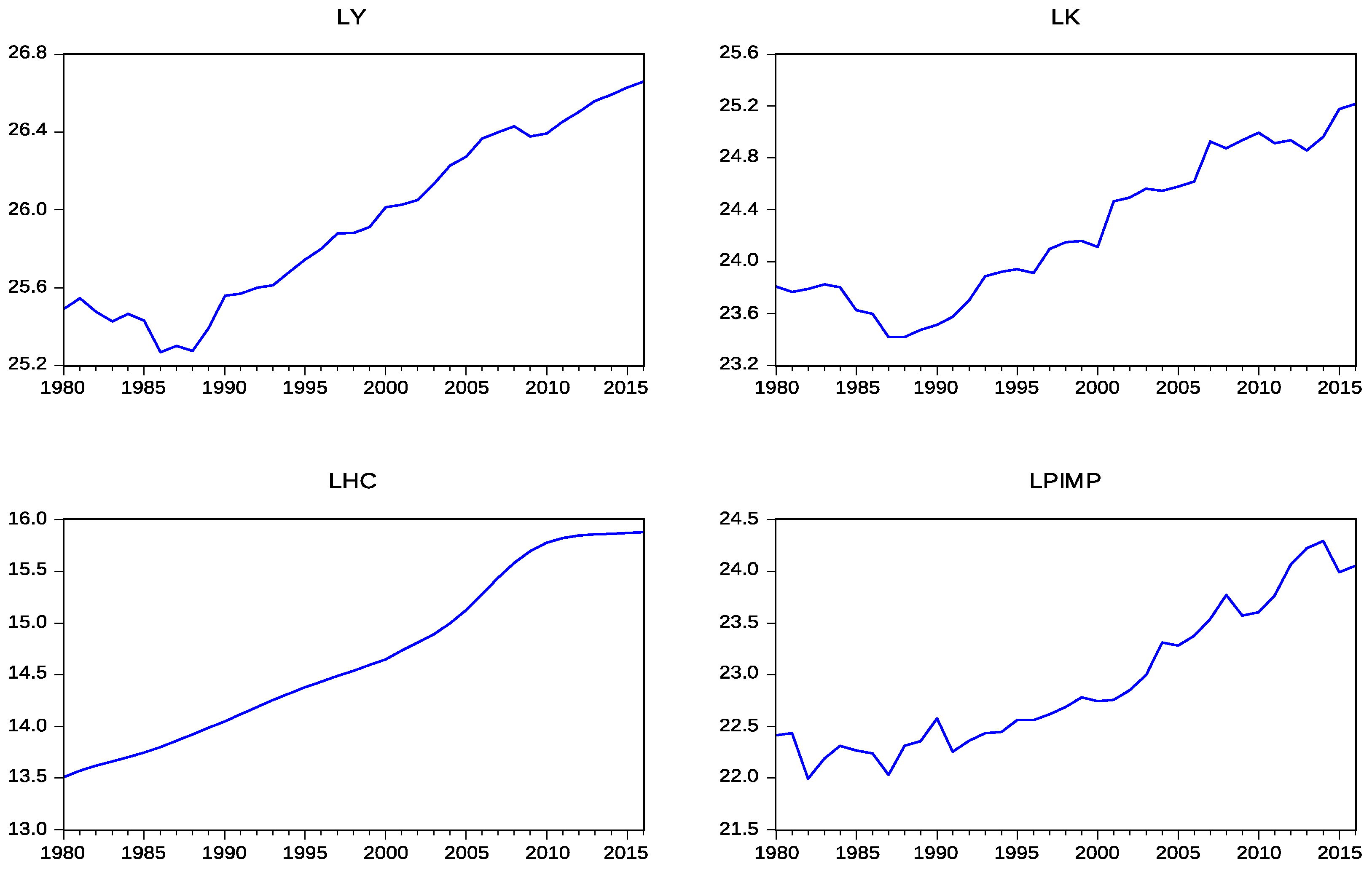
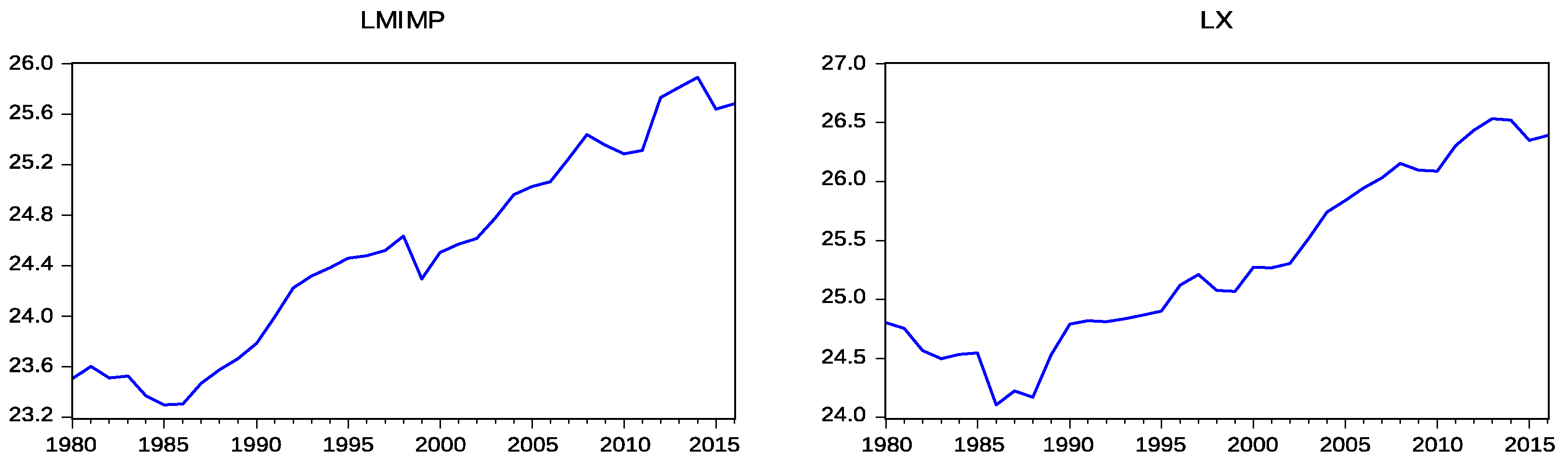
This research uses annual time series for the UAE from 1980 to 2016, obtained from national and international sources. Specifically, GDP (Y) and working age population (HC) are derived from the World Development Indicators-World Bank, while merchandise exports (X), primary imports (PIMP) and manufactured imports (MIMP) are obtained from the World Trade Organization. The data series for Gross Fixed Capital Formation (K) is taken from IMF, National Bureau of Statistics and World Bank. All the variables are expressed in logarithmic form and real terms, using the GDP deflator taken from the World Bank. The descriptive statistics and plots of the log-transformed data are shown in

Table 1. Descriptive statistics of the series for the period 1980–2016.

Statistics	LY	LK	LHC	LPIMP	LMIMP	LX
Mean	25.9	24.2	14.7	22.9	24.5	25.3
Median	25.9	24.1	14.5	22.7	24.5	25.1
Maximum	26.7	25.2	15.9	24.3	25.9	26.5
Minimum	25.3	23.4	13.5	22.0	23.3	24.1
Std. Dev.	0.4	0.6	0.8	0.7	0.8	0.7
Skewness	0.1	0.2	0.2	0.6	0.1	0.3
Kurtosis	1.6	1.6	1.7	2.0	1.8	1.8
Jarque-Bera	3.1	3.2	3.0	3.8	2.3	2.7
Probability	0.2	0.2	0.2	0.2	0.3	0.3
Observations	37	37	37	37	37	37

Source: Author’s calculation.

and Figure 1 respectively.

3.2. Methodology

This paper tests whether new technology embodied in imports causes expansion of merchandise exports with further effect on human capital accumulation and economic growth. It is assumed that the aggregate production of the economy can be expressed as a function of physical capital, human capital, primary imports, manufactured imports and merchandise exports:

Y_t = A_t K_t^α HC_t^β, 0 < α + β < 1

(1)

where Y_t denotes the aggregate production of the UAE economy at time t, A_t is the total factor productivity, while K_t and HC_t represent the physical capital stock and human capital respectively. The constants α and β are between zero and one, measuring the share of physical and human capital on income. In addition, it is assumed that the total factor productivity can be expressed as a function of primary imports, PIMP_t, manufactured imports, MIMP_t, merchandise exports, X_t and other exogenous factors C_t:

A_t = f(PIMP_t, MIMP_t, X_t, C_t) = PIMP_t^γ MIMP_t^δ X_t^ζ C_t

(2)

Combining Equations (1) and (2), the following equation is obtained:

Y_t = C_t K_t^α HC_t^β PIMP_t^γ MIMP_t^δ X_t^ζ

(3)

where α, β, γ, δ and ζ represent the elasticities of production with respect to the inputs of production: K_t, HC_t, PIMP_t, MIMP_t and X_t. After taking the natural logs of both sides of Equation (3), the following equation is obtained:

LY_t = c + αLK_t + βLHC_t + γLPIMP_t + δLMIMP_t + ζX_t + ε_t

(4)

where c is the intercept, α, β, γ, δ and ζ are constant elasticities, while ε_t is the error term, which reflects the influence of other factors that are not included in the model.

3.2.1. Unit Root Test

Before applying the Granger causality test it is important to ensure that the time-series variables are stationary, which means that they have a constant mean and variance. If the variables are not stationary, which is the most common case for macroeconomic variables, they can be made stationary by taking the first difference (ΔY_t = Y_t − Y_t−1). Initially, the Augmented Dickey-Fuller (ADF) test is conducted [26] in order to test for the presence of a unit root [27]. The ADF test is based on the following three equations:

$$\Delta Y_t={\alpha }_0+\gamma Y_{t-1}+{\alpha }_{2}t+{\sum }_{i=1}^p\beta i \Delta Y_{t-1}+{\epsilon }_t$$

(5)

$$\Delta Y_t={\alpha }_0+\gamma Y_{t-1}+{\sum }_{i=1}^p\beta i \Delta Y_{t-1}+{\epsilon }_t$$

(6)

$$\Delta Y_t=\gamma Y_{t-1}+{\sum }_{i=1}^p\beta i \Delta Y_{t-1}+{\epsilon }_t$$

(7)

where α₀ and α₂ represent the deterministic elements.

Equation (5) is a random walk with intercept and time trend, Equation (6) is a random walk with intercept only, while the last equation is a random walk [28]. In addition, the residuals are uncorrelated and identically distributed with zero mean and variance σ² {ε_t ~ ii(0, σ²) for t = 1, 2, …}. In each case, the null hypothesis is that γ = 0; H_o: unit root exists (variable is integrated of order one), while the alternative hypothesis is that γ < 0; H_a: unit root does not exist.

In addition, the Phillips-Perron unit root test is applied [29], which is a generalization of the DF procedure that allows for heteroskedasticity and serial correlation in the error terms [27].

This test involves the following equations:

Y_t = γ*₀ + γ*₁y_t−1 + μ_t

(8)

Y_t = γ*₀ + γ*₁y_t−1 + γ*₂ (t − T/2) + μ_t

(9)

where γ*₀ and γ*₂ are the deterministic elements, T is the number of observations, while μ_t is the error term. The procedure suggested by Dolado et al. [30] is followed in order to choose the appropriate equation for the above unit root tests.

This research also applies the test proposed by Kwiatkowski et al. [31], where the null hypothesis is a stationary process, as “not all series for which we cannot reject the unit root hypothesis are necessarily integrated of order one” [32] (p. 294). The Kwiatkowski-Phillips-Schmidt-Shin (KPSS) statistic is based on the residuals from the Ordinary Least Squares regression of y_t on the exogenous variables x_t (constant and time trend):

Y_t = δx_t′ + u_t

The KPSS statistic is defined as:

$$\mathrm{KPSS}={\sum }_{t}S{\left(t\right)}^2/(T^2{f}_0)$$

where f₀ is an estimator of the residual spectrum at frequency zero and S(t) is a cumulative residual function: S(t) = ${\sum }_{r=1}^t\widehat{u}$_r, based on the residuals û_t from the equation Y_t = δ x_t′ + u_t.

3.2.2. Cointegration Test

This paper applies the Johansen cointegration test [33,34] in order to confirm the existence of a long-run relationship between the variables. Johansen’s methodology estimates the cointegrating vectors using a maximum likelihood procedure, taking its starting point in the VAR of order p given by:

$$X_t=\mu +{\sum }_{i=1}^p{A}_i{X}_{t-i}+{\epsilon }_t$$

(10)

where X_t is a (n × 1) vector of variables that are I(1), μ is a (n × 1) vector of constants, A_i is an (n × n) matrix of parameters, while ε_t is a (n × 1) vector of random errors. Subtracting X_t−1 from each side of this equation and letting I be an (n × n) identity matrix, this VAR can be re-written as:

$$\Delta X_t=\mu +\Pi X_{t-1}+{\sum }_{i=1}^{p-1}{\Gamma }_i\Delta X_{t-i}+{\epsilon }_t$$

(11)

where

$${\Gamma }_i=-{\sum }_{j=i+1}^p{A}_j \mathrm{and} \Pi ={\sum }_{i=1}^p{A}_i-I$$

Γ_i and Π are the coefficient matrices, ΠX_t−1 is the error-correction term, while the coefficient matrix Π provides information about the long-run relationships among the variables. The number of the cointegrating vectors can be determined by using the likelihood ratio (LR) trace test statistic suggested by Johansen [33]. The LR trace statistic is adjusted for small sample size, as proposed by Reinsel and Ahn [35]. In particular, the LR trace statistic is adjusted by using the correction factor (T − n × p)/T, where T is the sample size, while n and p is the number of the variables and the optimal lag length respectively.

The LR trace statistic is given by the following equation:

$$J_{trace}=-T{\sum }_{i=r+1}^n\ln (1-\lambda i)$$

(12)

where T is the sample size and λ is the eigenvalue. The trace statistic tests the null hypothesis of at most r cointegrating vectors against the alternative hypothesis of n cointegrating vectors.

3.2.3. Short-Run Granger Causality Test

The Vector Autoregressive Model (VAR) model, which is developed by Sims [36], is used to investigate the existence of a short-run causality between technology embodied in imports, exports, human capital and economic growth in the UAE. In the VAR model, all variables are endogenous, while dummy variables can be included to ensure the stability of the model. The VAR model with six endogenous variables (LY_t, LK_t, LHC_t, LPIMP_t, LMIMP_t, LX_t) can be expressed as follows:

$$\begin{array}{c}L{Y}_t={\alpha }_{10}+{\sum }_{j=1}^p{\beta }_{1j} L{Y}_{t-j}+{\sum }_{j=1}^p{\gamma }_{1j} L{K}_{t-j}+ {\sum }_{j=1}^p{\delta }_{1j} LH{C}_{t-j}+{\sum }_{j=1}^p{\zeta }_{1j} LPIM{P}_{t-j}+ \\ {\sum }_{j=1}^p{\theta }_{1j} LMIM{P}_t{}_{-j}+{\sum }_{j=1}^p{\mu }_{1j} L{X}_t{}_{-j}+{\epsilon }_{1t}\end{array}$$

(13)

$$\begin{array}{c}L{K}_t={\alpha }_{20}+{\sum }_{j=1}^p{\beta }_{2j} L{Y}_{t-j}+{\sum }_{j=1}^p{\gamma }_{2j} L{K}_{t-j}+ {\sum }_{j=1}^p{\delta }_{2j} LH{C}_{t-j}+{\sum }_{j=1}^p{\zeta }_{2j} LPIM{P}_{t-j}+ \\ {\sum }_{j=1}^p{\theta }_{2j} LMIM{P}_t{}_{-j}+{\sum }_{j=1}^p{\mu }_{2j} L{X}_t{}_{-j}+{\epsilon }_{2t}\end{array}$$

(14)

$$\begin{array}{c}LH{C}_t={\alpha }_{30}+{\sum }_{j=1}^p{\beta }_{3j} L{Y}_{t-j}+{\sum }_{j=1}^p{\gamma }_{3j} L{K}_{t-j}+ {\sum }_{j=1}^p{\delta }_{3j} LH{C}_{t-j}+{\sum }_{j=1}^p{\zeta }_{3j} LPIM{P}_{t-j}+ \\ {\sum }_{j=1}^p{\theta }_{3j} LMIM{P}_t{}_{-j}+{\sum }_{j=1}^p{\mu }_{3j} L{X}_t{}_{-j}+{\epsilon }_{3t}\end{array}$$

(15)

$$\begin{array}{c}LPIM{P}_t={\alpha }_{40}+{\sum }_{j=1}^p{\beta }_{4j} L{Y}_{t-j}+{\sum }_{j=1}^p{\gamma }_{4j} L{K}_{t-j}+ {\sum }_{j=1}^p{\delta }_{4j} LH{C}_{t-j}+{\sum }_{j=1}^p{\zeta }_{4j} LPIM{P}_{t-j}+ \\ {\sum }_{j=1}^p{\theta }_{4j} LMIM{P}_t{}_{-j}+{\sum }_{j=1}^p{\mu }_{4j} L{X}_t{}_{-j}+{\epsilon }_{4t}\end{array}$$

(16)

$$\begin{array}{c}LMIM{P}_t={\alpha }_{50}+{\sum }_{j=1}^p{\beta }_{5j} L{Y}_{t-j}+{\sum }_{j=1}^p{\gamma }_{5j} L{K}_{t-j}+ {\sum }_{j=1}^p{\delta }_{5j} LH{C}_{t-j}+{\sum }_{j=1}^p{\zeta }_{5j} LPIM{P}_{t-j}+ \\ {\sum }_{j=1}^p{\theta }_{5j} LMIM{P}_t{}_{-j}+{\sum }_{j=1}^p{\mu }_{5j} L{X}_t{}_{-j}+{\epsilon }_{5t}\end{array}$$

(17)

$$\begin{array}{c}L{X}_t={\alpha }_{60}+{\sum }_{j=1}^p{\beta }_{6j} L{Y}_{t-j}+{\sum }_{j=1}^p{\gamma }_{6j} L{K}_{t-j}+ {\sum }_{j=1}^p{\delta }_{6j} LH{C}_{t-j}+{\sum }_{j=1}^p{\zeta }_{6j} LPIM{P}_{t-j}+ \\ {\sum }_{j=1}^p{\theta }_{6j} LMIM{P}_t{}_{-j}+{\sum }_{j=1}^p{\mu }_{6j} L{X}_t{}_{-j}+{\epsilon }_{6t}\end{array}$$

(18)

where LY_t, LK_t, LHC_t, LPIMP_t, LMIMP_t and LX_t represent the variables of the proposed model (Equation (4)), β_ij, γ_ij, δ_ij, ζ_ij, θ_ij and μ_ij are the regression coefficients, while p is the optimal lag length, selected by minimising the value of Schwartz Information Criterion (SIC).

Moreover, if the variables are found to be cointegrated, the following restricted VAR model (Vector Error Correction Model) can be used to find the direction of the causality:

$$\begin{array}{c}\Delta L{Y}_t={\sum }_{j=1}^p{\beta }_{1j} \Delta L{Y}_{t-j}+{\sum }_{j=1}^p{\gamma }_{1j} \Delta L{K}_{t-j}+{\sum }_{j=1}^p{\delta }_{1j} \Delta LH{C}_{t-j}+{\sum }_{j=1}^p{\zeta }_{1j} \Delta LPIM{P}_{t-j}+\\ {\sum }_{j=1}^p{\theta }_{1j} \Delta LMIM{P}_t{}_{-j}+{\sum }_{j=1}^p{\mu }_{1j} \Delta L{X}_t{}_{-j}-{\lambda }_{y}EC{T}_{t-}{}_1+{\epsilon }_{1t}\end{array}$$

(19)

$$\begin{array}{c}\Delta L{K}_t={\sum }_{j=1}^p{\beta }_{2j} \Delta L{Y}_{t-j}+{\sum }_{j=1}^p{\gamma }_{2j} \Delta L{K}_{t-j}+{\sum }_{j=1}^p{\delta }_{2j} \Delta LH{C}_{t-j}+{\sum }_{j=1}^p{\zeta }_{2j} \Delta LPIM{P}_{t-j}+\\ {\sum }_{j=1}^p{\theta }_{2j} \Delta LMIM{P}_t{}_{-j}+{\sum }_{j=1}^p{\mu }_{2j} \Delta L{X}_t{}_{-j}-{\lambda }_{k}EC{T}_{t-}{}_1+{\epsilon }_{2t}\end{array}$$

(20)

$$\begin{array}{c}\Delta LH{C}_t={\sum }_{j=1}^p{\beta }_{3j} \Delta L{Y}_{t-j}+{\sum }_{j=1}^p{\gamma }_{3j} \Delta L{K}_{t-j}+{\sum }_{j=1}^p{\delta }_{3j} \Delta LH{C}_{t-j}+{\sum }_{j=1}^p{\zeta }_{3j} \Delta LPIM{P}_{t-j}+\\ {\sum }_{j=1}^p{\theta }_{3j} \Delta LMIM{P}_t{}_{-j}+{\sum }_{j=1}^p{\mu }_{3j} \Delta L{X}_t{}_{-j}-{\lambda }_{hc}EC{T}_{t-}{}_1+{\epsilon }_{3t}\end{array}$$

(21)

$$\begin{array}{c}\Delta LPIM{P}_t={\sum }_{j=1}^p{\beta }_{4j} \Delta L{Y}_{t-j}+{\sum }_{j=1}^p{\gamma }_{4j} \Delta L{K}_{t-j}+{\sum }_{j=1}^p{\delta }_{4j} \Delta LH{C}_{t-j}+{\sum }_{j=1}^p{\zeta }_{4j} \Delta LPIM{P}_{t-j}+\\ {\sum }_{j=1}^p{\theta }_{4j} \Delta LMIM{P}_t{}_{-j}+{\sum }_{j=1}^p{\mu }_{4j} \Delta L{X}_t{}_{-j}-{\lambda }_{pimp}EC{T}_{t-}{}_1+{\epsilon }_{4t}\end{array}$$

(22)

$$\begin{array}{c}\Delta LMIM{P}_t={\sum }_{j=1}^p{\beta }_{5j} \Delta L{Y}_{t-j}+{\sum }_{j=1}^p{\gamma }_{5j} \Delta L{K}_{t-j}+{\sum }_{j=1}^p{\delta }_{5j} \Delta LH{C}_{t-j}+{\sum }_{j=1}^p{\zeta }_{5j} \Delta LPIM{P}_{t-j}+\\ {\sum }_{j=1}^p{\theta }_{5j} \Delta LMIM{P}_t{}_{-j}+{\sum }_{j=1}^p{\mu }_{5j} \Delta L{X}_t{}_{-j}-{\lambda }_{mimp}EC{T}_{t-}{}_1+{\epsilon }_{5t}\end{array}$$

(23)

$$\begin{array}{c}\Delta L{X}_t={\sum }_{j=1}^p{\beta }_{6j} \Delta L{Y}_{t-j}+{\sum }_{j=1}^p{\gamma }_{6j} \Delta L{K}_{t-j}+{\sum }_{j=1}^p{\delta }_{6j} \Delta LH{C}_{t-j}+{\sum }_{j=1}^p{\zeta }_{6j} \Delta LPIM{P}_{t-j}+\\ {\sum }_{j=1}^p{\theta }_{6j} \Delta LMIM{P}_t{}_{-j}+{\sum }_{j=1}^p{\mu }_{6j} \Delta L{X}_t{}_{-j}-{\lambda }_{x}EC{T}_{t-}{}_1+{\epsilon }_{6t}\end{array}$$

(24)

where Δ is the difference operator, β_ij, γ_ij, δ_ij, ζ_ij, θ_ij, μ_ij and λ_ij are the regression coefficients and ECT_t−1 is the error correction term derived from the cointegration equation.

After estimating the VAR model, diagnostic tests are conducted in order to determine whether the models are well specified and stable. These tests include the Jarque-Bera Normality test, the Breusch-Godfrey LM test for the existence of autocorrelation, the White Heteroskedasticity test, the Multivariate ARCH test and the AR roots stability test. In addition, the cumulative sum of recursive residuals (CUSUM) and the CUSUM of squares (CUSUMQ) tests are performed in order to detect parameter instability in the equations. Specifically, the CUSUM test detects systematic changes, while the CUSUMQ test detects haphazard changes in the parameters [37]. The CUSUM test proposed by Brown et al. [37] is based on the statistic:

$$W_t={\sum }_{k+1}^t{w}_t/s,\mathrm{where}t=k+1,\dots ,T$$

(25)

where s is the standard deviation of the recursive residuals (w_t), which is defined as:

w_t = (y_t − x_t′b_t−1)/(1 + x′_t (X_t−1′X_t−1)⁻¹ x_t)^1/2

where the numerator y_t − x′_t b_t−1 is the forecast error, b_t−1 is the estimated coefficient vector up to period t − 1 and x_t′ is the row vector of observations on the regressors in period t. The X_t−1 denotes the (t − 1) × k matrix of the regressors from period 1 to period t − 1. If the b vector changes, W_t tends to diverge from the zero mean value line, while if b vector remains constant, E(W_t) = 0. The test shows parameter stability if the cumulative sum of the recursive residuals lies inside the area between the two 5% significance lines, the distance between which increases with t.

The CUSUM of Squares test uses the square recursive residuals, w_t² and is based on the plot of the statistic:

$$S_t=({\sum }_{k+1}^t{w}_t{}^2)/({\sum }_{k+1}^T{w}_t{}^2),\mathrm{where}t=k+1,\dots ,T$$

(26)

The expected value of S_t, under the null hypothesis of b_t’s constancy, is E(S_t) = (t − k)/(T − k), which takes values from zero, at t = k, to unity at t = T. In this test the S_t are plotted together with the 5% critical lines and, as in the CUSUM test, movements inside the 5% significance lines indicate stability in the equation during the sample period.

After assessing the stability of the estimated parameters, this research applies the multivariate causality test [38,39]. The non-causality between disaggregated imports, merchandise exports, human capital and economic is examined by conducting the chi-square test.

3.2.4. Long-Run Granger Causality Test

This paper applies the modified version of the Granger causality test (MWALD) proposed by Toda and Yamamoto [40], involving the following model:

$$\begin{array}{c}L{Y}_t={\alpha }_{10}+{\sum }_{j=1}^{p+d_{max}}{\beta }_{1j} L{Y}_t{}_{-j}+{\sum }_{j=1}^{p+d_{max}}{\gamma }_{1j} L{K}_t{}_{-j}+{\sum }_{j=1}^{p+d_{max}}{\delta }_{1j} LH{C}_t{}_{-j}+\\ {\sum }_{j=1}^{p+d_{max}}{\zeta }_{1j} LPIM{P}_t{}_{-j}+{\sum }_{j=1}^{p+d_{max}}{\theta }_{1j} LMIM{P}_t{}_{-j}+\\ {\sum }_{j=1}^{p+d_{max}}{\mu }_{1j} L{X}_{t-j}+{\epsilon }_{1t}\end{array}$$

(27)

$$\begin{array}{c}L{K}_t={\alpha }_{20}+{\sum }_{j=1}^{p+d_{max}}{\beta }_{2j} L{Y}_t{}_{-j}+{\sum }_{j=1}^{p+d_{max}}{\gamma }_{2j} L{K}_t{}_{-j}+{\sum }_{j=1}^{p+d_{max}}{\delta }_{2j} LH{C}_t{}_{-j}+\\ {\sum }_{j=1}^{p+d_{max}}{\zeta }_{2j} LPIM{P}_t{}_{-j}+{\sum }_{j=1}^{p+d_{max}}{\theta }_{2j} LMIM{P}_t{}_{-j}+\\ {\sum }_{j=1}^{p+d_{max}}{\mu }_{2j} L{X}_{t-j}+{\epsilon }_{2t}\end{array}$$

(28)

$$\begin{array}{c}LH{C}_t={\alpha }_{30}+{\sum }_{j=1}^{p+d_{max}}{\beta }_{3j} L{Y}_t{}_{-j}+{\sum }_{j=1}^{p+d_{max}}{\gamma }_{3j} L{K}_t{}_{-j}+{\sum }_{j=1}^{p+d_{max}}{\delta }_{3j} LH{C}_t{}_{-j}+\\ {\sum }_{j=1}^{p+d_{max}}{\zeta }_{3j} LPIM{P}_t{}_{-j}+{\sum }_{j=1}^{p+d_{max}}{\theta }_{3j} LMIM{P}_t{}_{-j}+\\ {\sum }_{j=1}^{p+d_{max}}{\mu }_{3j} L{X}_{t-j}+{\epsilon }_{3t}\end{array}$$

(29)

$$\begin{array}{c}LPIM{P}_t={\alpha }_{40}+{\sum }_{j=1}^{p+d_{max}}{\beta }_{4j} L{Y}_t{}_{-j}+{\sum }_{j=1}^{p+d_{max}}{\gamma }_{4j} L{K}_t{}_{-j}+{\sum }_{j=1}^{p+d_{max}}{\delta }_{4j} LH{C}_t{}_{-j}+\\ {\sum }_{j=1}^{p+d_{max}}{\zeta }_{4j} LPIM{P}_t{}_{-j}+{\sum }_{j=1}^{p+d_{max}}{\theta }_{4j} LMIM{P}_t{}_{-j}+\\ {\sum }_{j=1}^{p+d_{max}}{\mu }_{4j} L{X}_{t-j}+{\epsilon }_{4t}\end{array}$$

(30)

$$\begin{array}{c}LMIM{P}_t={\alpha }_{50}+{\sum }_{j=1}^{p+d_{max}}{\beta }_{5j} L{Y}_t{}_{-j}+{\sum }_{j=1}^{p+d_{max}}{\gamma }_{5j} L{K}_t{}_{-j}+{\sum }_{j=1}^{p+d_{max}}{\delta }_{5j} LH{C}_t{}_{-j}+\\ {\sum }_{j=1}^{p+d_{max}}{\zeta }_{5j} LPIM{P}_t{}_{-j}+{\sum }_{j=1}^{p+d_{max}}{\theta }_{5j} LMIM{P}_t{}_{-j}+\\ {\sum }_{j=1}^{p+d_{max}}{\mu }_{5j} L{X}_{t-j}+{\epsilon }_{5t}\end{array}$$

(31)

$$\begin{array}{c}L{X}_t={\alpha }_{60}+{\sum }_{j=1}^{p+d_{max}}{\beta }_{6j} L{Y}_t{}_{-j}+{\sum }_{j=1}^{p+d_{max}}{\gamma }_{6j} L{K}_t{}_{-j}+{\sum }_{j=1}^{p+d_{max}}{\delta }_{6j} LH{C}_t{}_{-j}+\\ {\sum }_{j=1}^{p+d_{max}}{\zeta }_{6j} LPIM{P}_t{}_{-j}+{\sum }_{j=1}^{p+d_{max}}{\theta }_{6j} LMIM{P}_t{}_{-j}+\\ {\sum }_{j=1}^{p+d_{max}}{\mu }_{6j} L{X}_{t-j}+{\epsilon }_{6t}\end{array}$$

(32)

where p is the optimal lag length, selected by minimising the value of SIC, while d_max is the maximum order of integration of the variables in the model. The selected lag length (p) is augmented by the maximum order of integration (d_max) and the chi-square test is applied to the first p VAR coefficients.

4. Empirical Results

4.1. Unit Root Tests

Table 2. ADF, PP and KPSS test results at logarithmic level and first difference.

Variables	ADF	PP	KPSS
LY	−2.72 (a)	−2.72 (a)	0.13 *(a)
	[0]	{1}	{4}
DLY	−4.58 ***(b)	−4.59 ***(b)	0.26 (b)
	[0]	{2}	{2}
LK	−2.46 (a)	−2.44 (a)	0.14 *(a)
	[0]	{4}	{4}
DLK	−5.66 ***(b)	−5.66 ***(b)	0.32 (b)
	[0]	{0}	{0}
LHC	−2.30 (a)	−5.55 (c)	0.14 *(a)
	[2]	{4}	{4}
DLHC	−3.14 **(b)	−1.09 (c)	0.12 (b)
	[1]	{4}	{4}
LPIMP	−3.01 (a)	−2.95 (a)	0.21 **(a)
	[0]	{13}	{4}
DLPIMP	−6.07 ***(a)	−6.93 ***(b)	0.35 (b)
	[2]	{25}	{4}
LMIMP	−2.76 (a)	−2.72 (a)	0.70 **(b)
	[0]	{5}	{5}
DLMIMP	−5.47 (b)***	−5.45 ***(b)	0.09 (b)
	[0]	{5}	{5}
LX	−3.21 (a)	−3.48 *(a)	0.15 **(a)
	[0]	{8}	{4}
DLX	−4.92 (b)***	−4.59 ***(c)	0.23 (b)
	[0]	{0}	{2}

Notes: *, **, *** denote the rejection of the null hypothesis at 10%, 5% and 1% respectively. Numbers in [ ] corresponding to ADF test statistic are the optimal lags, chosen based on Schwarz Information Criterion (SIC). Bandwidth in { } (Newey-West automatic) using Bartlett kernel estimation method. The maximum lag length for the ADF test is found by rounding up P_max = [12* (T/100)^¼] = [12* (37/100) ^¼] ≅ 9 (see [41]). All the time series are tested for the unit root including intercept and trend ^(a), intercept only ^(b) and no intercept or trend ^(c). The letters in brackets indicate the selected model following Dolado et al. [30].

presents the results of the ADF, PP and KPSS unit root tests at levels and first differences. The ADF and PP test results indicate that the null hypothesis of non-stationarity cannot be rejected for all the variables at 5% significance level. In addition, the KPSS test results indicate that the null hypothesis of stationarity is rejected for all the variables at conventional levels of significance. In contrast, after taking the first difference of the variables, the null hypothesis of unit root can be rejected at 1% level of significance for all variables, except from the first-differenced series of LHC, which is found to be stationary at 5% significance level. In addition, the KPSS unit root test results indicate that the null hypothesis of stationary process cannot be rejected for all the variables at 5% significance level. Therefore, all the variables are non-stationary at level and stationary at first difference.

4.2. Cointegration Test

Table 3. Johansen’s Cointegration Test results.

Hypothesized Number of Cointegrating Equations	Adjusted Trace Statistic	Critical Value 1%
r = 0	121.09 ***	111.01
r ≤ 1	78.08	84.45

Note: Critical values are taken from Osterwald-Lenum [42]. The model includes a restricted constant (Model selection based on Pantula Principle [43]). The lag length for the cointegration test is determined by minimizing the Schwarz Information Criterion (SIC), while the diagnostic tests reveal that the residuals are multivariate normal, homoscedastic and there is no evidence of serial correlation. *** indicate rejection at 1% significance level.

presents the cointegration test results. The null hypothesis of no cointegration is rejected at 1% significance level, indicating the existence of one cointegrating equation.

The cointegrating equation is estimated after normalizing on LY and the following long-run relationship is obtained. The absolute t-statistics are reported in the parentheses:

LY_t = 0.20***LK_t + 0.18***LHC_t − 0.15***LPIMP_t + 0.07LMIMP_t
(3.79)   (3.54)   (2.63)   (1.38)
+ 0.34***LX_t + 11.57***
(4.70)   (15.58)

(33)

From Equation (33) a 1% increase in physical capital leads to a 0.20% increase in real GDP, while a 1% increase in human capital raises real GDP by 0.18%. In addition, a 1% increase in manufactured imports and exports can lead to an increase in real GDP by 0.07% and 0.34% respectively. However, manufactured imports are found to be insignificant at 5% significance level. In contrast, real GDP decreases by 0.15% in response to a 1% increase in primary imports. These results suggest that physical capital, human capital and exports enhance economic growth in the UAE, through investments in advanced technology and knowledge spillover effects, while primary imports and manufactured imports have a significant negative effect and an insignificant positive effect respectively on economic growth in the long-run.

4.3. Granger Causality in VECM Framework

The VECM is estimated with the inclusion of two impulse dummy variables for the years 1986 and 2009, as the CUSUMQ plots of the initially estimated ECMs for economic growth and human capital show evidence of structural instability. The estimated ECMs without the inclusion of the dummy variables are not reported here, but are available upon request. The short-run Granger causality results for the UAE are reported in

Table 4. Short-run Granger causality test.

Dependent Variable	Source of Causation
	ΔLYt	ΔLKt	ΔLHCt	ΔLPIMPt	ΔLMIMPt	ΔLXt	ALL
	χ2 (1)	χ2 (1)	χ2 (1)	χ2 (1)	χ2 (1)	χ2 (1)	χ2 (5)
ΔLYt	-	0.19	5.41 **	3.68 **	1.62	1.13	11.05 **
ΔLKt	1.43	-	0.70	4.14 **	2.13	0.01	15.30 ***
ΔLHCt	0.29	0.00	-	0.40	2.18	1.09	5.04
ΔLPIMPt	3.23 *	0.25	2.11	-	0.07	6.42 ***	8.78
ΔLMIMPt	0.04	0.14	3.43 *	0.06	-	1.32	8.92
ΔLXt	1.52	0.12	8.53 ***	6.98 ***	3.01*	-	16.60 ***

Note: *, ** and *** indicate significance at 10%, 5% and 1% significance level respectively. The lag length for the VECM is determined by minimizing the Schwarz Information Criterion (SIC). The diagnostic tests for the VECM model show that there is no problem of serial correlation, while the residuals are multivariate normal and homoskedastic. In addition, the stability of the VECM is confirmed by calculating the inverse roots of the characteristic AR polynomial. Df in parentheses.

.

The results of the Granger causality test show that primary imports Granger-cause economic growth at 5% significance level, while economic growth Granger-causes primary imports at 10% significance level, indicating that a bi-directional causal relationship exists between these variables. These results show that an increase in primary imports, encourages domestic-substituting firms to innovate in order to be more competitive, expanding their investments in new technology, improving productivity and economic growth. In return, further economic growth creates new needs, which cannot be covered by the domestic production, leading to a further increase in the level of imports.

Moreover, the null hypothesis of non-causality from human capital to economic growth can be rejected at a 5% significance level. At the same time, the null hypothesis of non-causality from human capital to manufactured imports and the null hypothesis of non-causality from human capital to exports can be rejected at 10% and 1% respectively. These findings show that human capital positively contributes to the efficient use of imported technology and exports expansion, improving productivity and the level of economic growth.

In contrast, the null hypothesis that manufactured imports do not cause economic growth and the null hypothesis that exports do not cause economic growth cannot be rejected at any conventional significance level.

However, an indirect short-run causality runs from manufactured imports and human capital to economic growth, through exports and primary imports. In particular, manufactured imports and human capital Granger-cause exports at a 10% and 1% significance level respectively. At the same time, exports Granger-cause primary imports at a 1% significance level and primary imports Granger-cause economic growth at a 5% significance level.

These results indicate that an increase in manufactured imports can cause an increase in export-oriented production, through the adoption of advanced technology. In parallel, exports expansion causes an increase in some categories of primary imports, which are used as inputs of production for manufactured exports. Therefore, imports positively affect economic growth, through technology and expansion of manufactured exports, as this category of exports offers knowledge spillover effects and positive externalities to non-exports sectors, leading to further economic growth [24,25].

In addition, the results show that all the variables in the model jointly Granger-cause economic growth in the short-run at a 5% significance level, while all variables in the model jointly cause physical capital accumulation and exports at 1% significance level. The results confirm the importance of these factors in the models.

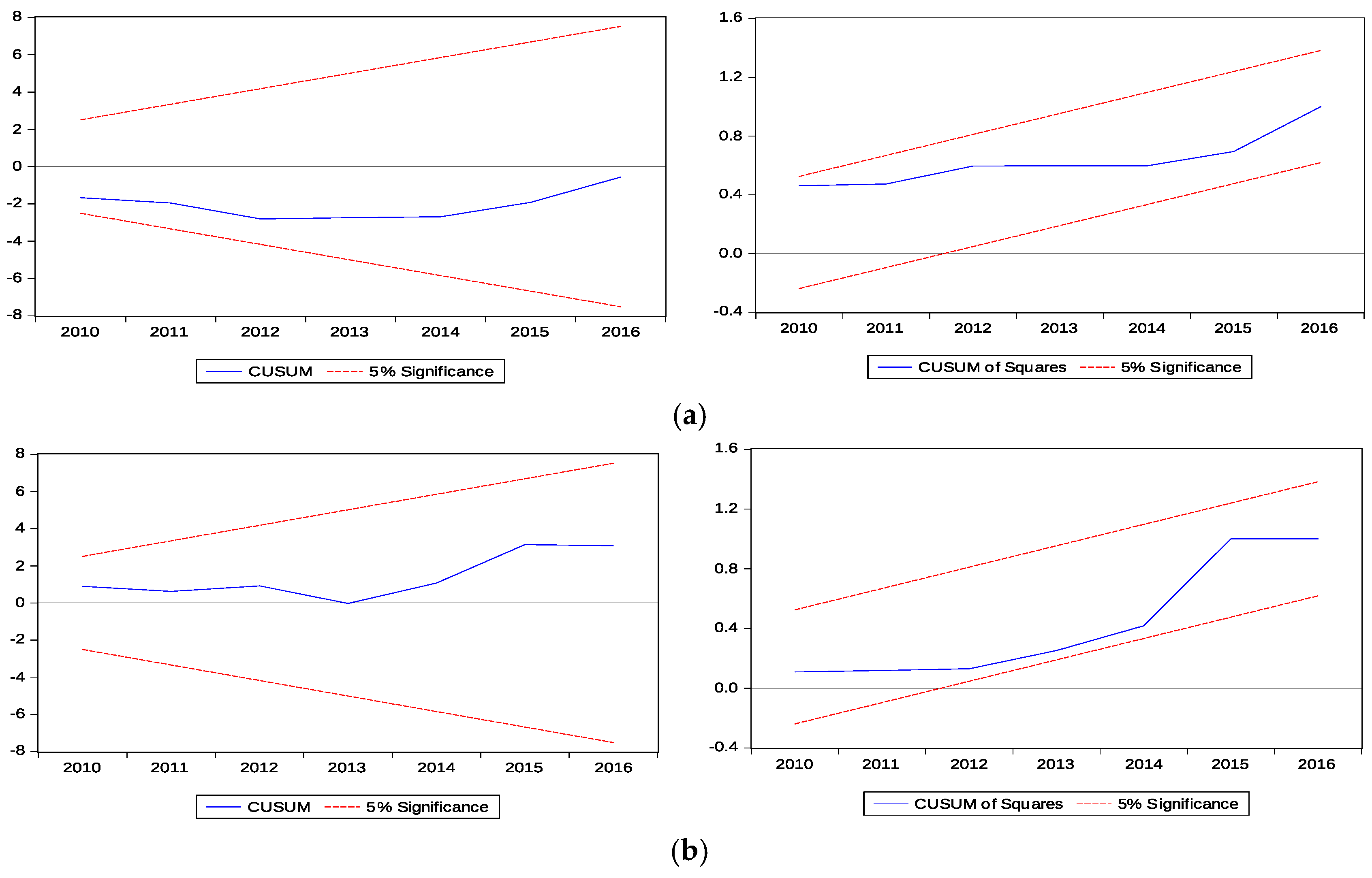
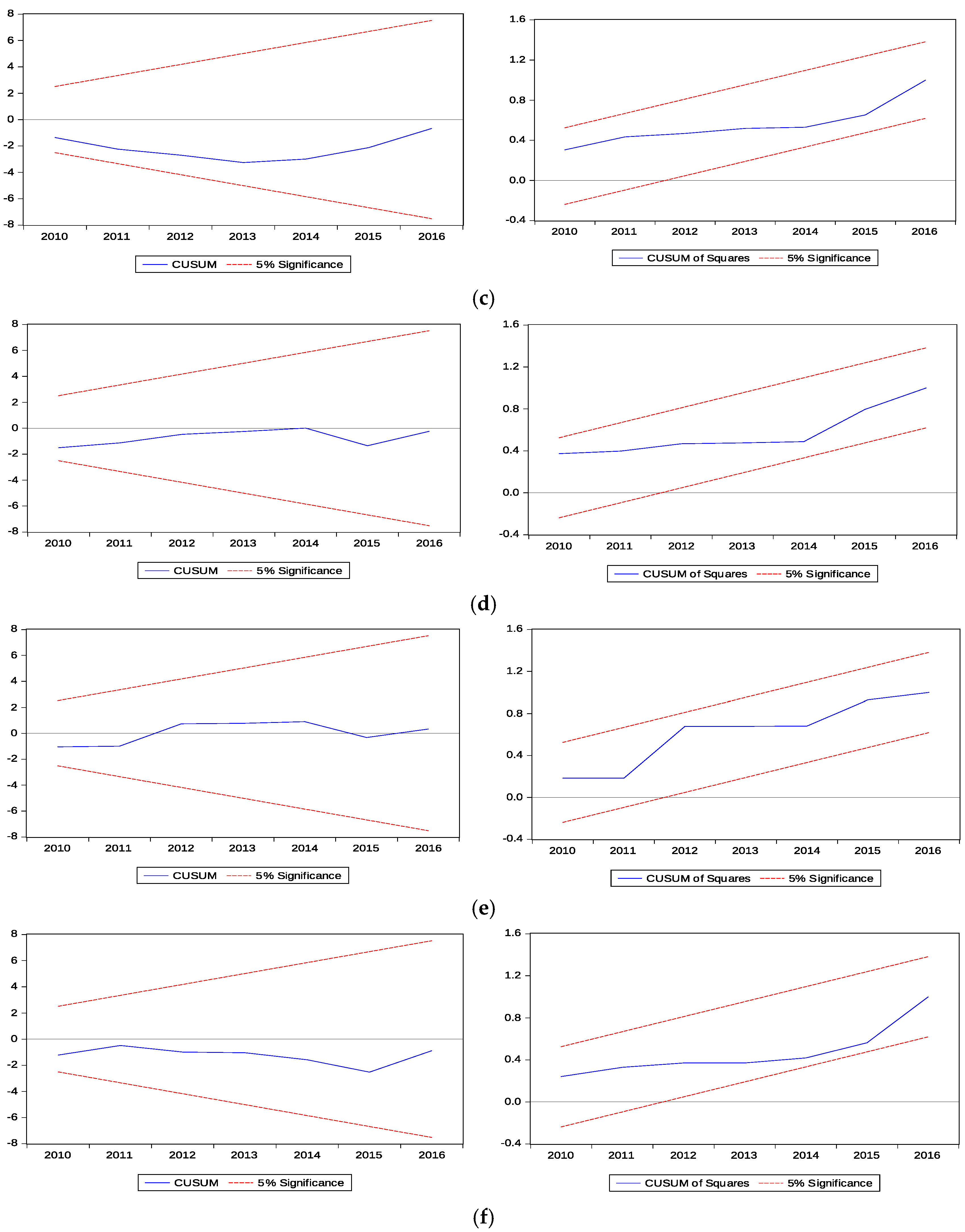
Since the aim of this research focuses on the relationship between trade, technology, human capital and economic growth, emphasis is placed on the structural stability of the parameters of the estimated error correction models for LY_t, LK_t, HC_t, PIMP_t, MIMP_t and X_t (Equations (19)–(24)). The CUSUM plots (Figure 2) for the estimated ECMs show that there is no movement outside the 5% critical lines. Therefore, the estimated ECMs, including the impulse dummy variables for the years 1986 and 2009, are stable. Thus, there is no reason to test for the presence of a third structural break.

4.4. Toda-Yamamoto Granger Causality Test

The optimal lag length for the VAR model, based on SIC (p = 2), is augmented by the maximum order of integration (d_max = 1) and the Wald tests are applied to the first p VAR coefficients. The MWALD test does not provide evidence of either ILG or ELG hypothesis in the long-run, while no causality runs from primary imports, manufactured imports or exports to human capital. However, the results show that LY_t, LK_t, HC_t, PIMP_t, MIMP_t and X_t jointly Granger cause physical capital in the long-run. The results are presented in

Table 5. Granger Causality based on Toda-Yamamoto procedure.

Dependent Variable	Source of Causation
	LYt	LKt	LHCt	LPIMPt	LMIMPt	LXt	ALL
	χ2 (2)	χ2 (2)	χ2 (2)	χ2 (2)	χ2 (2)	χ2 (2)	χ2 (10)
LYt	-	1.42	0.15	0.45	1.90	1.34	6.16
LKt	2.96	-	0.52	1.10	0.86	3.78	22.67 ***
LHCt	0.26	2.68	-	0.65	0.65	0.34	8.48
LPIMPt	0.02	3.23	1.25	-	0.24	2.77	15.25
LMIMPt	1.18	0.29	2.60	4.14	-	0.01	12.01
LXt	1.82	1.21	2.71	1.82	1.39	-	10.52

Note: *** indicates significance at 1% significance level. The diagnostic tests for the select VAR(p) model prior to the application of the Toda-Yamamoto procedure show that there is no problem of serial correlation, while the residuals are multivariate normal and homoskedastic. Df in parentheses.

.

5. Conclusions

The empirical results indicate the existence of a direct bi-directional causality between primary imports and economic growth in the short-run. In this case, an increase in primary imports encourages domestic-substituting firms to innovate in order to be more competitive, expanding their investments in new technology, improving productivity and economic growth. In return, further economic growth creates new needs, leading to imports expansion. Therefore, the adoption of advanced technology in UAE takes place via R&D investments and innovation efforts to compete in foreign markets.

In contrast, there is no evidence to support the existence of direct causality from manufactured imports and exports to economic growth in the short-run. However, an indirect short-run causality runs from manufactured imports to economic growth, through exports and primary imports. These results indicate that an increase in manufactured imports causes an increase in export-oriented production, through the adoption of advanced technology. In parallel, exports expansion causes an increase in primary imports, as this category of imports is essential for the expansion of UAE exports and especially for manufactured exports. It should be noted that expansion of manufactured exports can cause further economic growth, as this category of exports offers knowledge spillover effects and other externalities to non-exports sectors.

It should be noted that no causality runs in the short-run from merchandise exports and disaggregated imports to human capital. However, human capital directly causes economic growth, manufactured imports and merchandise exports in the short-run. Therefore, emphasis should be placed on policies that encourage human capital, imports and exports, as these factors directly or indirectly cause economic growth in the short-run, due to technology transfer and knowledge diffusion.

As far as the long-run causality is concerned, empirical results do not provide evidence of either ILG or ELG hypothesis, while no causality runs from merchandise exports and disaggregated imports to human capital. These results show that other factors than merchandise exports or technology embodied in manufactured imports contribute to economic growth and human capital accumulation in the long-run. Further disaggregation of imports or exports could help in identifying the source of long-run economic growth, as aggregate measures may mask the different causal effects that subcategories of exports or imports can have. These results do not mean that technology does not contribute to sustainable economic growth and improvement of human capital in the long-run, as this research uses technology embodied in imports and not a proxy that can measure endogenous technology development and innovation, such as patents.

It should be recognized that this study might have a number of limitations. First, this study uses the working age population as a proxy for human capital, due to the fact that data related to the labor force, education attainment for population 25+ or patent applications of residents and non-residents was not obtainable for the period 1980–2016. Second, the fact that the UAE is an oil-producing country may limit the generalizability of the findings to resource-abundant countries. Researching the causal relationship between trade, technology transfer, human capital and economic growth in the UAE could help in designing future policies for accelerating and sustaining economic growth in less developed resource-abundant countries.