Identifying Economic Growth Convergence Clubs and Their Influencing Factors in China

Abstract

Balanced and coordinated economic development across regions is a critical goal of regional economic development and new-type urbanization in China. However, few studies have examined economic growth convergence clubs at the county level. To extend the research on convergence clubs, this research applies a log t convergence test and a dynamic spatial ordered probit model (DSOP) to endogenously identify economic growth convergence clubs in counties and to examine the influence of initial states and structures on club convergence probability. The study sample covers 2286 counties of China from 1992 to 2010. The results show significant convergence club patterns at the county levels, resulting in the gradual formation of six convergence clubs. The DSOP estimation results show that per capita fixed assets, population density, and industrialization have promoted convergence club formation to varying degrees.

1. Introduction

Since the late 20th century, classical economic growth theories have been questioned and challenged. The traditional economic growth model presented by Solow [1] has been heavily criticized due to issues of endogeneity and variable omission [2]. The neoclassical economic convergence models presented in Barro and Sala-i-Martin [3,4] and Mankiw et al. [5] also fail to determine paths of economic transition and individual heterogeneity [6]. Other economic growth theories suggest that economies with similar initial structures cannot develop different degrees of overall convergence [7]. Therefore, questions concerning the existence of overall economic growth convergence persist. However, although the economy as a whole cannot achieve convergence, convergence phenomena may still be found within economic groups with similar structural characteristics [6]. The notion that economic groups with similar initial characteristics can realize a steady state of equilibrium through a relatively balanced developmental path forms the premise of the so-called “convergence club” hypothesis [8,9,10,11]. The gradual movement toward a steady state of equilibrium promotes the development of convergence clubs [7]. It indicates that economies with semblable structural characteristics may be able to converge to dissimilar steady state equilibria, although they have different initial conditions. Therefore, a common growth path is not unexpected for a group of semblable economies, only if their initial states are likely to initiate the same long-run equilibrium [12]. In this sense, the convergence club method can provide a more authentic and micromesh view of regional economic growth than the traditional convergence method [13].

In that context, the goal of this paper is to identify convergence clubs and to investigate which influencing factors trigger the formation of convergence clubs across counties in China. We used two steps to explore the answer. The first step is to endogenously make convergence clubs of counties. The second step is to examine the influence of driving factors, including structural features and initial states for club counties.

Our contribution to the field of convergence studies is threefold. First, unlike the previous literature that uses traditional regressing methods, we use a novel convergence test, the log t test, developed by Phillips and Sul [6], to identify convergence clubs and to address issues of individual heterogeneity, economic structure, heterogeneous effects, and economic transition and convergence paths for China, a rapidly growing country in transition. Despite there having been numerous studies regarding convergence, the abovementioned issues remain largely underexplored.

Second, unlike the previous literature that describes the observed clubs, we try to examine the relative importance of different growth-influencing factors, including structural features and initial states, for a county’s club membership in China using a dynamic spatial ordered probit model (DSOP). Through the study, we provide a feasible path to distinguish the role of initial conditions and structural characteristics for the forming mechanism of convergence clubs. In particular, we try to test whether the probability of belonging to a certain convergence club is dependent upon a county’s labor participation rate, investment in fixed assets per capita, human capital, population density, and industrial structure.

Finally, from a spatial scale perspective, unlike the previous literature that uses the provincial level as a basic unit for the identification of convergence clubs (e.g., Herrerias and Ordonez [14]), we use 2286 Chinese counties’ panel data to examine convergence clubs to provide more practical and precise information for convergence clubs in China. For large countries such as China, convergence clubs exist not only across regions and provinces but also within counties. We believe that regional disequilibrium and uncoordinated development caused by rapid economic growth may be more serious at the county level. Meanwhile, in local places, neighboring counties may easily form a steady-state club. County-level studies offer more helpful information not only on macro spatial distributions of convergence clubs but also on patterns of local and regional spatial and temporal heterogeneity. Thus, studies of county-level economic growth convergence clubs can more tangibly guide intermediate microeconomic regional policies [15,16].

2. Literature Review

To test the convergence club hypothesis, scholars have conducted research on convergence club identification and the development of the appropriate econometric tools. The regression tree analysis method is commonly used for identification purposes. Durlauf and Johnson identified country groups through a regression tree analysis based on initial income and human capital levels and concluded that country convergence speeds within groups are significantly higher than those of overall samples [17]. Fischer and Stirbock tested the convergence club phenomena in Europe using spatial econometric models and following Durlauf’s research [13]. Corrado, Martin, and Weeks also developed the multivariate stationary test as a mature convergence club identification algorithm and identified the European regional economic growth convergence club [18]. New economic geography theory, initiated by Krugman [19,20], has also been used to examine similar issues. In addition, studies of economic agglomeration, which is closely related to convergence club formation, form two research areas: spatial economic agglomeration and economic growth [14]. Existing studies have focused on convergence club formation in China; however, different models and different datasets have yielded mixed results that are sometimes sharply different. Yao and Zhang [21] used the unit root test, the non-equilibrium index, the cross-section data procedure, and the panel data method to confirm the existence of geo-economic clubs of provincial economic development in China, for example. Zhang, Liu, and Yao [22] using 40-year time-series data from eastern, central, and western China, verified the convergence issue in income per capita. Hao [23] also confirmed convergence club formation in regional economic development throughout China. Pan [24] proposed the existence of stages of club convergence throughout China’s 30 years of reform. However, Liu, Wei, and Li [25] introducing a Gini coefficient decomposition method, found no convergence clubs in China. Therefore, there is no consensus concerning whether convergence clubs have been present in China. However, despite these contrasts, little empirical research has used the log t test to examine provincial or smaller scales economic development convergence clubs in China.

The existing identification methods of convergence club cannot address issues of individual heterogeneity, economic structure, heterogeneous effects, economic transition, and convergence paths. Phillips and Sul [6] thus proposed an innovative economic convergence test method (log t convergence test) and various test methods for convergence club phenomena. Test methods are advantageous in that they do not meet the requirement that each time series is cointegrated; they therefore permit individual economies to be transitionally divergent [12]. In fact, an absence of co-integration does not translate into lacking convergence [6]. Test methods also endogenously reveal behavioral patterns of economic transition, such as those involving convergence to a steady state of equilibrium, divergence, and club convergence. Given its advantages, numerous scholars have applied this method. Applications have included the identification of regional economic growth convergence clubs [12,26,27], financial development convergence pattern analysis [28], and energy market convergence club analysis [29].

Although the log t method can be used on the identification of convergence clubs, researchers cannot confirm how these clubs were formed. Specifically, it is difficult to assess which influencing variables lead to the formation of the multiplicity of the steady state of equilibrium [12]. If the formation of convergence clubs is solely motivated by structural characteristics, the evidenced patterns may be explained wrongly as club convergence in cases where conditional convergence is applied. Therefore, it is hard to differentiate between club convergence and conditional convergence in practice relying only on convergence club identification [26]. Therefore, factors influencing convergence club ownership possibilities must also be addressed. However, little empirical study has been conducted on this issue. The works by Bartkowska and Riedl [12] and von Lyncker and Thoennessen [30] are the main exception. Bartkowska and Riedl [12] use ordered logit regression models for the European NUTS-2 (Nomenclature of Territorial Units for Statistics-level 2) regional economic growth convergence club to investigate whether initial conditions are responsible for club formation. Von Lyncker and Thoennessen [30] examine club convergence in income per capita in 194 European NUTS-2 regions and use an ordered response model to estimate the effects of initial and structural conditions, as well as geographic factors on the formation of club convergence.

With respect to method, the ordered response model is an effective tool for detecting the influencing factors of convergence club classification. However, for regional economic development research, numerous scholars believe that spatial effects must be controlled to avoid biased outcomes [31,32,33]. Fruitful spatial econometrics studies examine spatial effects. The introduction of spatial effects into the ordered response model has also received considerable attention from scholars. Anselin [33] provided a systematic summary for the spatial probit model. Using a spatial autoregressive (SAR) model based on expectation-maximization (EM) algorithms, Mcmillen [34] first estimated the Probit model. Subsequently, Lesage [35] used the Gibbs sampling method to estimate the discrete response model with the spatial error term. Smith and Lesage [36] extended this research using Bayesian techniques to integrate spatial effects and completed an empirical test. The generalized method of moments (GMM) was applied to the discrete response model with spatial effects [37]. However, numerous previous studies are based on the binary response model [38]. Few studies apply spatial ordered response models. Wang [39] and Wang and Kockelman [38,40] proposed a dynamic spatial ordered Probit model (DSOP) using Bayesian estimation techniques and used this model for data simulation and land development intensity analysis. This model is one of the more mature spatial ordered probit models. Therefore, the present study uses the DSOP model recommended by Wang and Kockelman [38] to identify the influencing factors of economic convergence club members at the county level in China.

3. Materials and Methods

We use two methods for identifying convergence clubs and analyzing which influencing factors drive the development of convergence clubs across counties in China. First, we use the analysis of log t convergence test developed by Phillips and Sul [6]. In this paper, we extend this method to test the convergence clubs in China at the county level. Second, a dynamic spatial ordered probit regression model was applied to examine the forming mechanism of convergence clubs, that is, identifying the influences of different driving factors. In this part, the two methodologies are presented, and the sample data and data resources are described.

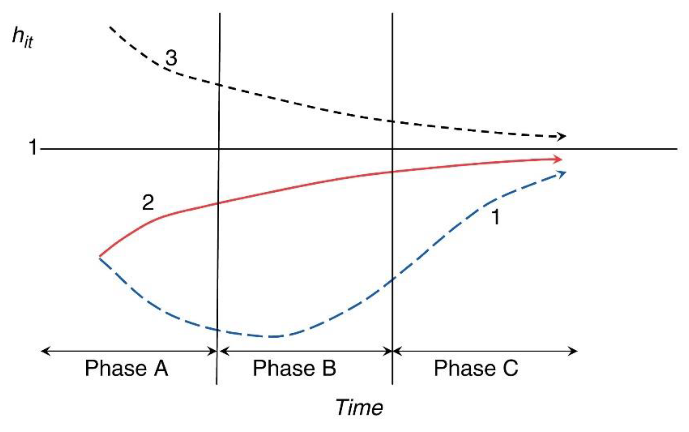
3.1. Log t Convergence Test

In this section, we briefly describe the method developed by Phillips and Sul [2,6]. The log t model considers individual heterogeneity based on the neoclassical economic growth theoretical framework. The specification of panel logarithmic GDP per capita under this framework can be expressed as follows:

$$\log y_{it}={\phi }_i{\mu }_t+{\epsilon }_{it}$$

(1)

where φ_i denotes the characteristic unit, μ_t represents common factors, and ε_it is the error term. There is a time-varying factor indication that can arise from the classical panel data representation as follows:

$$\log y_{it}=({\phi }_i+\frac{{\epsilon }_{it}}{{\mu }_t}){\mu }_t={\delta }_{it}{\mu }_t$$

(2)

where δ_it contains the error term and the unit-specific component and therefore indicates heterogeneity features that vary over time. Thus, Equation (1) describes individual behaviors of log y_it with common factors μ_t and two unit-specific components (φ_i and ε_it). Equation (2) reflects changes in the dependent variable in the form of the estimation of the common growth path (μ_t) and economic unit ratio (δ_it). Hence, Equation (2) can determine the convergence phenomenon by verifying whether the load value of factor δ_it is convergent. To determine time and economic growth transition heterogeneity, Phillips and Sul [2] developed time heterogeneity technologies by allowing technological development A_it to follow a path format A_it = A_i0 exp (x_itt). The log y_it transition path under heterogeneity technologies can be shown as follows:

$$\log y_{it}=\log {\tilde{y}}_i^{\ast }+\log A_{i0}+[\log {\tilde{y}}_{i0}-\log {\tilde{y}}_i^{\ast }]e^{-{\beta }_{it}t}+x_{it}\times t$$

(3)

where $\log {\tilde{y}}_{i0}$ and $\log {\tilde{y}}_i^{\ast }$ represent log GDP per capita at the initial and steady stages. β_it is the adjustment speed overtime.

Equation (3) can be expressed in the following form (same as Equation (2)):

$$\log y_{it}=\log {\tilde{y}}_i^{\ast }+\log A_{i0}+[\log {\tilde{y}}_{i0}-\log {\tilde{y}}_i^{\ast }]e^{-{\beta }_{it}t}+x_{it}\times t=a_{it}+x_{it}\times t={\delta }_{it}{\mu }_t$$

(4)

where x_it represents the technological improvement parameter and μ_t represents factor ratios in common growth elements. These elements may represent the common technology levels of industrial and scientific innovation or internet technologies. Therefore, the dynamic factor equation δ_itμ_t includes both common economic growth elements μ_t and an individual transition element δ_it, which can be used to estimate the transition path of the common steady stage. During the transition stage, the transition of the individual elements δ_it depends on the convergence speed parameter β_it, the technological improvement parameter x_it, the initial technology level, and the steady level determined by a_it.

To simulate the transition parameter δ_it, the relative transition parameter h_it is constructed through the following equation:

$$h_{it}=\frac{\log y_{it}}{N^{-1}{\displaystyle \sum _{i=1}^N\log y_{it}}}=\frac{{\delta }_{it}}{N^{-1}{\displaystyle \sum _{i=1}^N{\delta }_{it}}}$$

(5)

where h_it denotes the transformation path of i economic unit compared with the cross-sectional average level. Hence, the common growth path element is eliminated, because the method calculates individual economic behaviors in relation to other economic units. Furthermore, this approach allows one to estimate the distance of unit i from the common growth path μ_t. Under convergence conditions, all economic units followed the same transformation path; when t → ∞, h_it → 1. The cross-sectional variance of h_it can be expressed as $V_t^2=N^{-1}{\sum }_i{(h_{it}-1)}^2$, which shall converge to 0. When convergence does not occur, V_t may be positive and indicate the presence of classic convergence clubs.

To construct the null hypothesis of the economic growth convergence, Phillips and Sul [6] presented a semi-parametric model as follows:

$${\delta }_{it}={\delta }_i+\frac{{\sigma }_i{\xi }_{it}}{L(t)t^{\alpha }}{\delta }_{it}={\delta }_i+\frac{{\sigma }_i{\xi }_{it}}{L(t)t^{\alpha }}$$

(6)

where δ_i is constant, σ_i is the heterogeneity degree parameter, ξ_it is iid (0,1) across i but weakly dependent over t, L(t) is a slowly varying function for which L(t) → ∞ as t → ∞, and α is the decline rate. This formula guarantees that δ_it converges to δ_i for all α ≥0. Hence, it can be seen as a null hypothesis.

The convergence null hypothesis can be expressed as follows:

$$H_0:{\delta }_i=\delta \&\alpha \ge 0.$$

(7)

And it is tested against the alternative $H_A:{\delta }_i\ne \delta$ for all i or $\alpha <0$. Therefore, even if the other methods fail, the log t test can be used to identify economic behaviors that were traditionally thought to be divergent.

Phillips and Sul [6] presented a limiting format of cross-sectional variance h_it based on Equation (6):

$$V_t^2~\frac{A}{L{(t)}^2{t}^{2\alpha }},t\to \infty ,A>0.$$

(8)

Therefore, the convergence test regression equation can be written as

$$\log \left(\frac{V_1^2}{V_t^2}\right)-2\log L(t)=a+b\log t+u_t,t=[rT],[rT]+1,\dots ,T$$

(9)

where $r\in (0,1)$. According to the Monte Carlo simulation, the L(t) = log t and r = 0.3 setting when the sample scope T is smaller than 50 is quite reasonable. The critical parameter b is associated with α. They indicated that the fitted value of log t is $\widehat{b}=2\widehat{\alpha }$(where $\widehat{\alpha }$ is the estimated value of α in H₀). A unilateral t-test robust to heteroskedasticity and autocorrelation (HAC) is used to test the inequality of null hypothesis $\alpha \ge 0$. If $t_{\widehat{b}}<-1.65$ (the conventional robust t statistic for the coefficient $\widehat{b}$, significant at the 5% level), the null hypothesis of convergence is rejected.

However, rejecting the null hypothesis of convergence does not mean that there is no convergence in the subgroups of the panel, because different situations can be met. For example, it is still possible that the presence of convergence clusters in the full panel follow steady-state growth paths [6]. Hence, it is necessary to identify whether there are convergence clubs in the full panel. In this regard, Phillips and Sul [6] suggested the following steps to identify the convergence clubs.

Step 1: Sample units (counties) are processed following reversed order in the full panel.

Step 2: Selecting the first k highest counties (log GDP per capita) in the panel to compose the core group G_k for some N > k ≥2, we then perform the log t regression and calculate the convergence test statistic $t_k=t(G_k)$ for the core group G_k. Based on a standard $k^{*}=\arg \underset{k}{\max }\left\{t_k\right\}$ subject to $\min \left\{t_k\right\}>-1.65$, the number of counties in the core group is determined by maximizing t_k over k. Condition $\min \left\{t_k\right\}>-1.65$ can help to ensure that the null hypothesis of convergence is valid for each k. If all counties were assigned a single convergence club, then the number of convergence clubs is N. In contrast, if there are two or more convergence clubs, the cluster will have a size smaller than N. If $\min \left\{t_k\right\}>-1.65$ is not supported for k = 2, then the highest counties in the core group can be excluded from each subgroup, and new subgroups are formed. This procedure can be implemented again and again to meet the condition. If the condition is not supported for all such sequential pairs, then we reason that those counties were divergent.

Step 3: We set $G_{k^{*}}^c$ as a complemental group to the core group $G_{k^{*}}$, brought one of the remaining counties in $G_{k^{*}}^c$ at a time to the k* members of the core group $G_{k^{*}}$, and performed the log t regression. If $\widehat{t}>c$, the counties were contained in the convergence club, where c is some chosen critical value ($\widehat{t}$ represents the t-statistic for this regression). Usually, we used the Monte Carlo method to identify the choice of the critical value. This step was repeated for the rest of counties and shaped the first sub-convergence club. We needed to operate the log t regression for this first sub-convergence club and make sure that $t_{\widehat{b}}>-1.65$ for the entire group. If not, the critical value, c, needed to be raised to improve the identifying ability of the log t test, and we repeated this procedure until the emergence of first sub-convergence group.

Step 4: We shaped a sub-group for all counties for which $\widehat{t}<c$ in Step 3 and performed the log t regression for this sub-group to verify whether $t_{\widehat{b}}>-1.65$ and this cluster converged. In that case, we could infer that there were two convergent clubs in the panel. If not, we continued to perform Steps 1–3 on this sub-group to ensure whether there was a smaller sub-group that shaped a convergence club. If there was no k in Step 2 for which $t_{\widehat{b}}>-1.65$, it drew the conclusion that the rest of the counties were divergent.

Convergence club identification is realized through GAUSS9.0. GAUSS codes were sourced from Phillips and Sul [2]. The panel logarithmic GDP per capita of 2286 counties was an input data to identify the economic growth convergence clubs.

3.2. Dynamic Spatial Ordered Probit Regression Model

The dynamic spatial ordered probit regression model that considers spatial autocorrelation extends the scope of the existing research [36,41]. Wang [39] and Wang and Kockelman [38] discussed the settings and estimation methods of the DSOP model in detail.

The DSOP model settings are as follows:

$$U_{ikt}=\lambda U_{ikt-1}+{X^{\prime }}_{ikt}\beta +{\theta }_i+{\epsilon }_{ik},t=1,\dots ,T$$

(10)

where i is the clubs (I = 1,…,M), k denotes individual counties inside the clubs (k = 1,…,n_i), and t is the time period. In another expression, there are M counties/neighborhoods, each of which includes n_i observations, and the observation total is ${\displaystyle \sum _{i=1}^M{n}_i=N}$. λ is the time autocorrelation estimated coefficient. Each unit is observed over T time period, producing a total observation number of NT. U_ikt is the potential response variable (unobserved) in this paper. The range of values was from 1 to 6, corresponding to 6 identified convergence clubs. However, the sixth club included only 94 counties, thus, we merged clubs 5 and 6 into one club. The final response variables ranged from 1–5 for unit k from county i during time t. U_ikt−1 is one period lagged, dependent variables of the unobserved dependent variable. The residual contains two parts, θ_i, which absorbs all common yet random elements for observations with county i, while the rest of the random component is caught by individual effect ε_ik, which is the heteroskedasticity with variance v_i (i.e., var (ε_ik) = v_i). After the U_ikt−1 were controlled, the error terms are correlated and identically distributed. X_ikt is a Q × 1 vector of independent variables, and β is a series of corresponding estimated parameters. In this paper, the explanatory variables include the labor participation rate (LABOR), the investment in fixed assets per capita (LNFIX), human capital (LNHUM), population density (LNDEN), and the proportion of the added value of the secondary industry in GDP (IND).

These settings reflect the spatial autocorrelations with counties. A spatial autocorrelation state can be represented as follows:

$${\theta }_i=\rho {\displaystyle \sum _{j=1}^M{w}_{ij}{\theta }_j}+u_i,i=1,\dots ,M$$

(11)

where spatial weight w_ij represents spatial contiguity, which can be calculated from the adjacency or distance between counties. The degree of neighboring impact is represented by the spatial effect parameter ρ. u_i aims to absorb any regional effects, and it is supposed to be iid normally distributed, with a mean of zero and a common variance of σ². Therefore, the spatial effect vector can be written as follows:

$$\theta =\rho W\theta +u\hspace{1em}or\hspace{1em}\theta ={(I-\rho W)}^{-1}u,u~N(0,{\sigma }^2{I}_M).$$

(12)

The regional effect vector will be a function of the weight matrix W, which has zero on its diagonal and is composed of purely exogenous elements w_ij, as follows:

$$W=\left[\begin{array}{cccc}0& w_{12}& \cdots & w_{1M}\\ w_{21}& 0& \cdots & w_{2M}\\ ⋮& ⋮& \ddots & ⋮\\ w_{M1}& w_{M2}& \cdots & 0\end{array}\right].$$

(13)

For an ordered probit, the observed response variable, y_ikt, can be expressed as follows:

$$y_{ikt}=s\mathrm{if}{\gamma }_{s-1}<U_{ikt}<{\gamma }_s,\mathrm{for}s=1,\dots ,S.$$

(14)

The observed variable is a censored form of the latent variable, and the possible outcomes are integers between 1 and S (In this paper, S = 5, corresponding to the number of identified convergence clubs). The latent variable U_ikt can change within the unknown boundaries ${\gamma }_0<{\gamma }_1<\dots <{\gamma }_{S-1}<{\gamma }_S$; γ₀ tends to be an infinite negative, whereas γ_S tends to be an infinite positive. If the constant term is involved in the explanatory variables, γ₁ also is normalized to equal 0. The probabilities of these S outcomes can be expressed as follows:

$$\begin{array}{l}\mathrm{Pr}(y_{ikt}=1|X_{ikt})=\mathsf{\Phi }\left(\frac{{\gamma }_1-\lambda U_{ikt-1}-X_{ikt}\beta -{\theta }_i}{{\upsilon }_i^{1/2}}\right)-\mathsf{\Phi }\left(\frac{{\gamma }_0-\lambda U_{ikt-1}-X_{ikt}\beta -{\theta }_i}{{\upsilon }_i^{1/2}}\right)\\ \mathrm{Pr}(y_{ikt}=2|X_{ikt})=\mathsf{\Phi }\left(\frac{{\gamma }_2-\lambda U_{ikt-1}-X_{ikt}\beta -{\theta }_i}{{\upsilon }_i^{1/2}}\right)-\mathsf{\Phi }\left(\frac{{\gamma }_1-\lambda U_{ikt-1}-X_{ikt}\beta -{\theta }_i}{{\upsilon }_i^{1/2}}\right)\\ \hspace{1em}\hspace{1em}\hspace{1em}⋮\\ \mathrm{Pr}(y_{ikt}=S|X_{ikt})=\mathsf{\Phi }\left(\frac{{\gamma }_S-\lambda U_{ikt-1}-X_{ikt}\beta -{\theta }_i}{{\upsilon }_i^{1/2}}\right)-\mathsf{\Phi }\left(\frac{{\gamma }_{S-1}-\lambda U_{ikt-1}-X_{ikt}\beta -{\theta }_i}{{\upsilon }_i^{1/2}}\right)\end{array}$$

(15)

where Ф (•) is the cumulative distribution function of the standard normal distribution.

The resulting likelihood function can be expressed as follows as follows:

$$\mathrm{Pr}(y|U,\gamma )={\displaystyle \prod _{t=1}^T{\displaystyle \prod _{i=1}^M{\displaystyle \prod _{k=1}^{n_i}{\displaystyle \sum _{s=1}^S\vartheta }}}}(y_{ikt}=s)\cdot \mathrm{Pr}(y_{ikt}=s|X_{ikt})$$

(16)

where y, U, and γ are the vector of y_ikt, U_ikt, and γ_s, respectively. ϑ (A) is an indicator function that equals 1 when event A is true (and 0 otherwise).

The DSOP model estimation method functions within the Bayesian framework, in which each parameter corresponds to prior and posterior distributions. The posterior distribution is calculated using the Markov chain Monte Carlo method. Wang [39] describes this estimation method in detail.

Detailed calculations of the convergence club influencing factors were performed through Matlab 2012a, and the codes were developed by Wang and Kockelman [38] and Wang [39].

3.3. Sample Data and Preliminary Processing

A county is a basic administrative unit of China, used to organize economic activities and administrative management, to support economic life, social life and cultural life, to connect the rural–urban interflow, and to promote rural economic development and industrialization. In fact, the stabilization and development of counties is a basis to boost the political stability, social progress, and economic prosperity of China. Using the county as a basic unit provides a finer analysis of convergence clubs compared with using a prefecture or province. Moreover, using the county as a basic unit helps investigate the inner regional equality within prefectures or provinces. There are three administrative units at the county level in China: the county (including autonomous counties), the county-level city, and the urban district. Data on counties and county-level cities were primarily derived from the China Statistical Yearbook for Regional Economy (2002–2011) and Social and Economic Statistical Yearbook of China’s County and City (2000–2011). Data for 1992, 1995, and 1999 were primarily drawn from the 2000 Statistical Yearbook. Because the China Statistical Yearbook for Regional Economy (2002–2011) does not include urban district data, these data were primarily derived from the China City Statistical Yearbook (1993–2011). Missing data for specific years and regions were supplemented using statistical yearbooks of various provinces (including districts and directly controlled municipalities from 1993–2011). Following basic data and data accessibility requirements, we constructed a socioeconomic database for Chinese counties for 1992–2010 (for data prior to 2000, only data for 1992, 1995, and 1999 were relatively complete for statistical reasons) that accounts for 2286 county units. The reason for choosing 1992 as the start of the study period is mainly that the socialist market economy system began to develop in China in 1992. Another reason is that China started publishing the county-level statistical data in 1992.

To examine the regional differences in the influencing factors behind the formation of convergence clubs, we used China’s four regions as our regression analyses sample to explore influencing factor effects on different regions. According to the classification methods of the National Bureau of Statistics of China (NBSC), the four main regions are defined as follows: the eastern region covers (580 sampled cities and counties) Beijing, Tianjin, Hebei, Shandong, Jiangsu, Zhejiang, Shanghai, Fujian, Guangdong, and Hainan; the central region covers (573 sampled cities and counties) Shanxi, Henan, Anhui, Hubei, and Hunan, Jiangxi; the western region covers (951 sampled cities and counties) Inner Mongolia, Shaanxi, Ningxia, Gansu, Chongqing, Sichuan, Guizhou, Yunnan, Guangxi, Qinghai, Tibet, and Xinjiang; and the northeastern region covers (182 sampled cities and counties) Liaoning, Jilin, and Heilongjiang.

Here, five explanatory variables, including the labor participation rate (LABOR), the investment in fixed assets per capita (LNFIX), the human capital (LNHUM), the population density (LNDEN), and the proportion of the added value of the secondary industry in GDP (IND), are used as input data to estimate the effects of these variables on the formation of convergence clubs. LABOR is a variable used to investigate the condition of the labor participation rate (%) in the entire society. The natural logarithm of the investment in fixed assets per capita (LNFIX) represents the investment level of each county. LNHUM reflects human capital levels, using the natural logarithm of the enrollment in regular secondary schools as the proxy variable. The natural logarithm of population density (LNDEN) variable is used to investigate the effects of population aggregation. IND is the proportion of the added value of the secondary industry in GDP (%) (see

Table 1. Variables and sources (Source: modified by the authors).

Variable	Definition	Sources
GDP per capita (Yuan)	The value of all final goods and services produced divided by the resident population at year-end; the GDP data were deflated to the constant price of 1992 using a GDP deflator obtained from the National Bureau of Statistics of China.	China Regional Statistical Yearbook (2002–2011), China City Statistical Yearbook (1993–2011), China Statistical Yearbook (1993–2011).
Labor participation rate (%)	The proportion of people who are either employed or are actively looking for work in the total population.	Social and Economic Statistical Yearbook of China’s County and City (2000–2011), China City Statistical Yearbook (1993–2011).
Investment in fixed assets per capita (Yuan)	The social fixed asset investment divided by the population; the investment data were deflated to the constant price of 1992 by price index for investment in fixed assets.	China Regional Statistical Yearbook (2002–2011), China City Statistical Yearbook (1993–2011), China Statistical Yearbook (1993–2011).
Enrollment of regular secondary schools (Students/10,000 population)	Enrollment of regular secondary schools divided by 10,000 population.	Social and Economic Statistical Yearbook of China’s County and City (2000–2011), China City Statistical Yearbook (1993–2011).
Population density (Population/km2)	Population divided by total land area (area in square km).	China Regional Statistical Yearbook (2002–2011), China City Statistical Yearbook (1993–2011).
Proportion of the added value of the secondary industry in GDP (%)	GDP in the secondary industry as a share of total GDP, used to characterize industrialization levels.	China Regional Statistical Yearbook (2002–2011), China City Statistical Yearbook (1993–2011).

for detailed description).

Table 2. Descriptive statistics of variables (Source: modified by the authors).

Variables	Sample	Mean	Std. Dev.	Min	Max	Obs.
GDP per capita (Yuan)	China	11,247.0	14,850.0	16.3	368,704.0	2286 × 14
	Eastern China	17,497.9	18,702.0	654.3	368,704.0	580 × 14
	Central China	9239.4	10,195.3	414.9	294,426.5	573 × 14
	Western China	8383.6	13,420.0	16.3	288,043.1	951 × 14
	Northeast China	12,620.5	14,324.5	545.6	197,383.7	182 × 14
Labor participation rate (%)	China	51.0	12.0	10.5	76.0	2286 × 14
	Eastern China	53.7	11.1	14.8	76.0	580 × 14
	Central China	52.1	11.5	13.6	68.0	573 × 14
	Western China	50.3	11.7	11.2	65.0	951 × 14
	Northeast China	46.2	15.3	10.5	71.0	182 × 14
Investment in fixed assets per capita (Yuan)	China	5285.0	10,805.0	1.0	399,902.0	2286 × 14
	Eastern China	7300.0	10,884.0	1.0	162,755.0	580 × 14
	Central China	4319.3	7104.2	1.0	111,809.8	573 × 14
	Western China	4591.4	12,535.2	1.0	399,902.0	951 × 14
	Northeast China	5531.5	9514.7	6.1	94,587.2	182 × 14
Enrollment of regular secondary schools (Students/10,000 population)	China	589.0	204.0	1.0	9041.7	2286 × 14
	Eastern China	646.0	170.0	1.0	4198.0	580 × 14
	Central China	645.1	176.7	81.6	8751.0	573 × 14
	Western China	526.1	215.5	3.9	9041.7	951 × 14
	Northeast China	555.2	220.9	132.4	4139.0	182 × 14
Population density (Population/km2)	China	377.0	539.0	0.3	14,052.0	2286 × 14
	Eastern China	605.0	712.0	1.0	14,052.0	580 × 14
	Central China	487.2	550.4	5.9	5903.0	573 × 14
	Western China	190.7	283.0	0.3	4315.7	951 × 14
	Northeast China	283.4	519.6	1.6	10,172.5	182 × 14
Proportion of the added value of the secondary industry in GDP (%)	China	38.0	17.0	1.2	92.0	2286 × 14
	Eastern China	44.6	13.9	5.3	92.0	580 × 14
	Central China	41.3	15.0	3.0	90.0	573 × 14
	Western China	31.8	17.5	1.2	89.0	951 × 14
	Northeast China	36.4	16.9	2.5	91.0	182 × 14

lists the descriptive statistics results for six key variables.

Graphic data were primarily drawn from the National Geomatics Center of China (NGCC, http://ngcc.sbsm.gov.cn) and the data sharing infrastructure of Earth System Science (www.geodata.cn). Due to continuous changes in administrative divisions, we needed to adjust administrative units. To ensure the consistency of the counties over several years, a backtracking method, in which administrative division codes were reviewed from the final year to the first year, was applied. To ensure regional continuity over time and to render the data order consistent with the basic characteristics of panel data, we compared the characteristics of counties for each year and adjusted counties that experienced changes. Because GDP is a current price measure that must be deflated to improve the accuracy of the data, we deflated the county GDP index for all of the studied years to the level recorded in 1992.

Basic spatial weight matrix calculation data included latitude and longitude coordinates for the central points of the counties listed on a nationwide county map provided by the NGCC. Coordinate information extraction and application was realized through ESRI ArcGIS 10.1. We used the Matlab 2012a platform to convert coordinate information into a spatial weight matrix via xy2cont coding (http://www.spatial-econometrics.com/), finally obtaining a 2286 × 2286 adjacency matrix.

4. Results

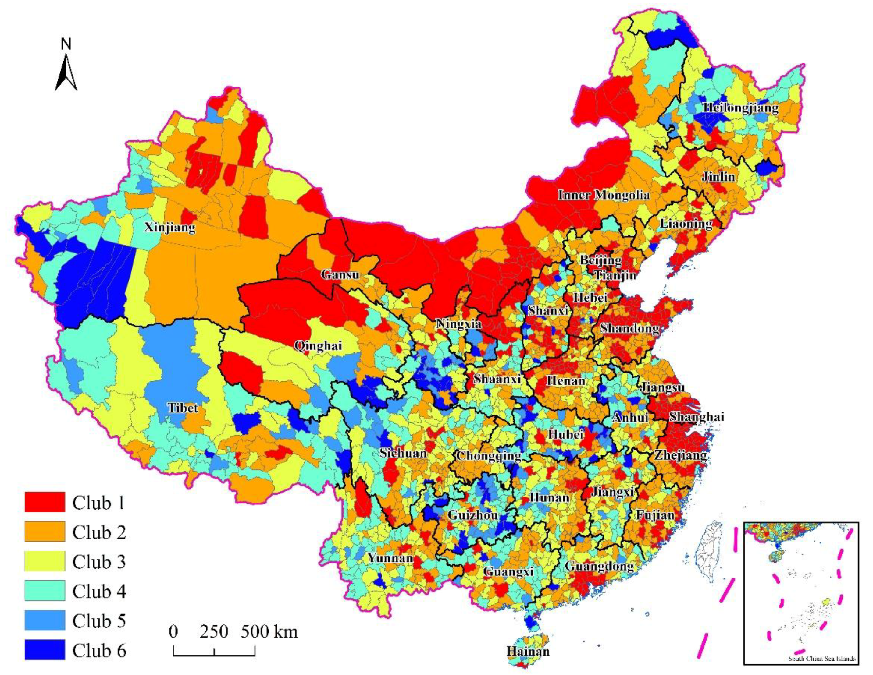
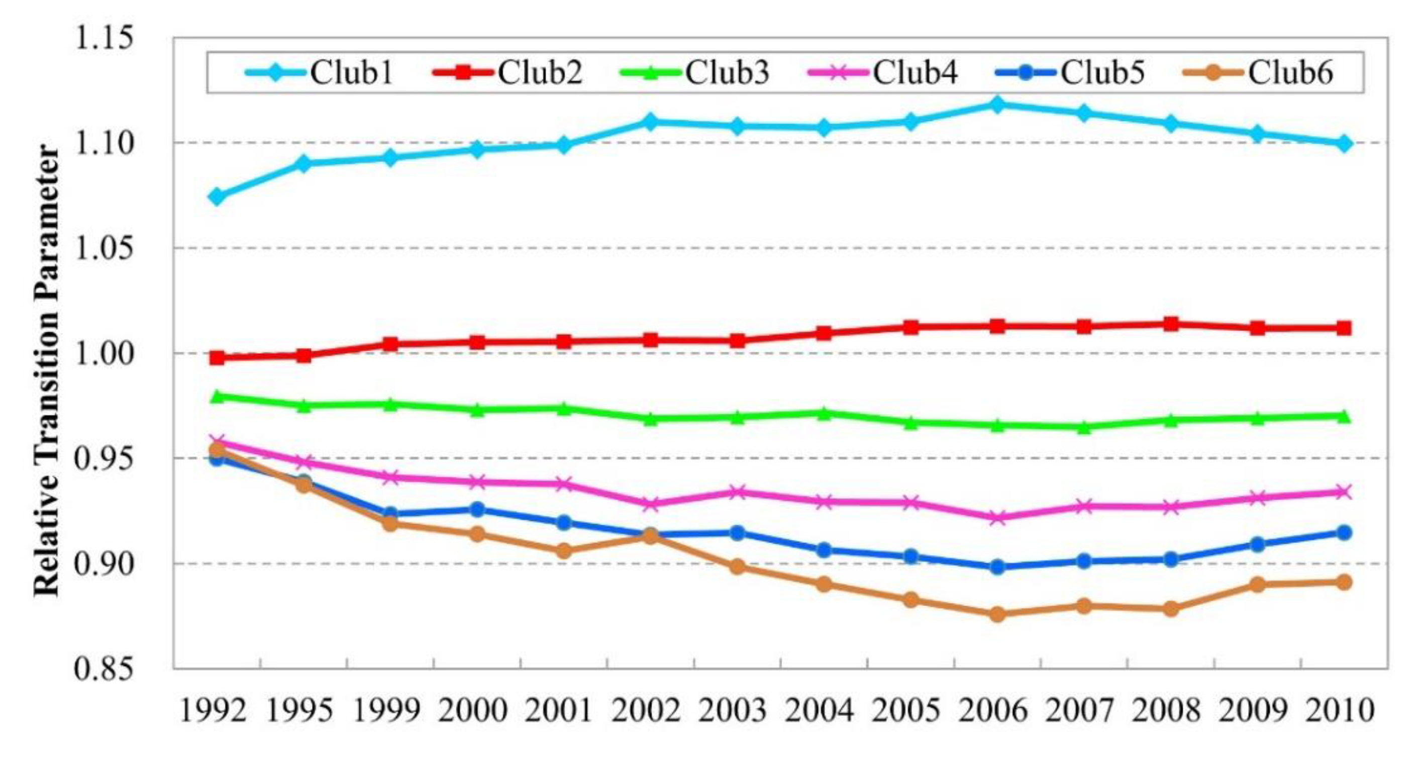
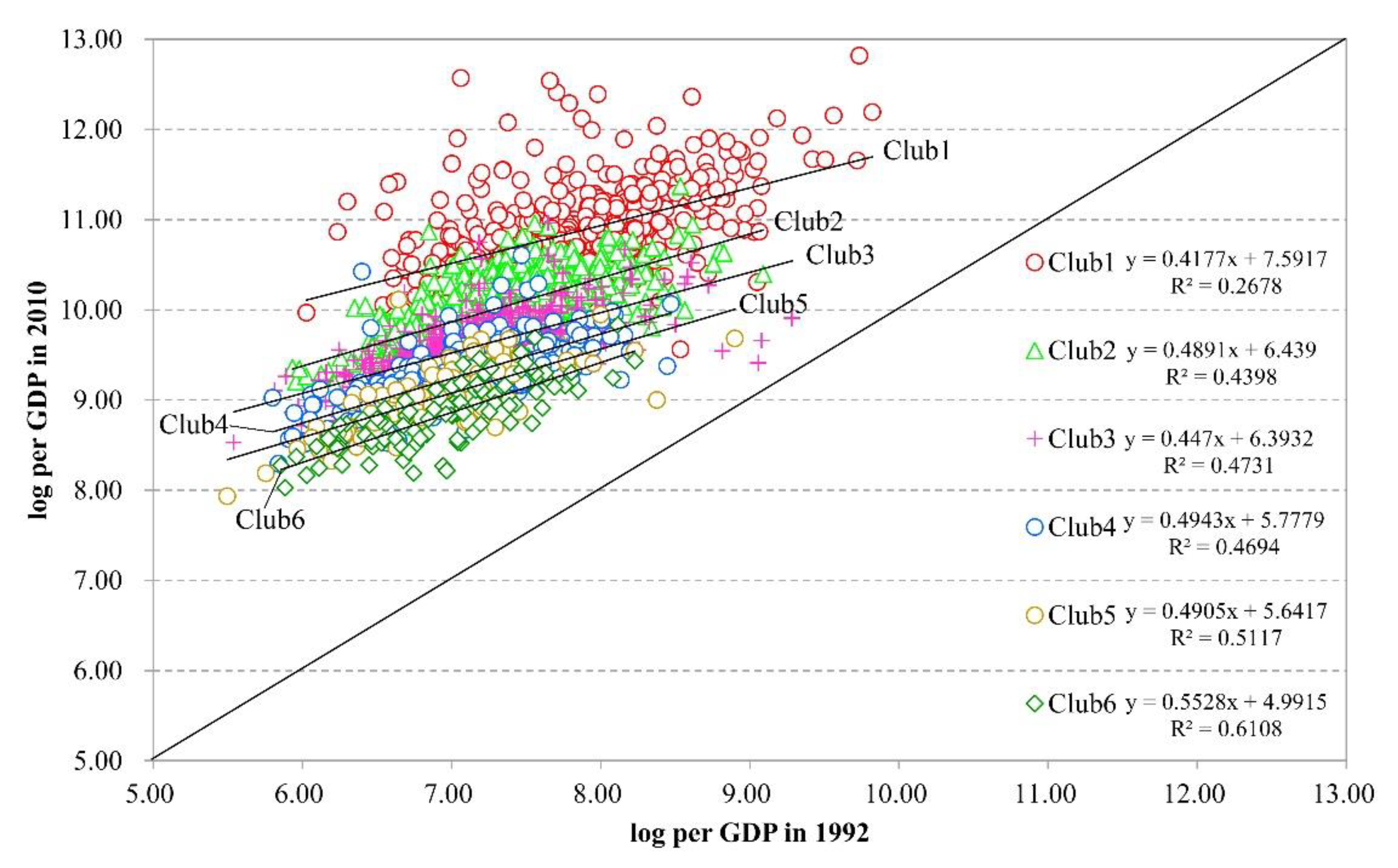
4.1 Convergence Club Identification

In applying the log t test for the identification of economic growth convergence clubs in data from 2286 counties across China, the convergence was not found for the total sample at the 5% significant level ($\widehat{b}$ was significantly less than zero, t-statistic was −81.526; i.e., the null hypothesis of global convergence was rejected at the 5% significance level). We believed that there was no steady state of county economic convergence in China. Therefore, we used the convergence club identification method to examine convergence clubs.

Table 3. Convergence club classification (Source: modified by the authors).

Initial Club		Tests of Club Merging					Final Club		GDP Per Capita (1992–2010)
Club	$\widehat{\mathit{b}}$ (SE of $\widehat{\mathit{b}}$)	$\widehat{\mathit{b}}$ (SE of $\widehat{\mathit{b}}$)					Club	$\widehat{\mathit{b}}$ (SE of $\widehat{\mathit{b}}$)
Total sample [2286][M1]	−0.945 (0.014)								11,247
Club 1 [491][M2]	0.259 (0.017)	Club 1 + 2					Club 1 [491][M3]	0.259 (0.017)	16,647
		−0.564 * (0.015)
Club 2 [718][M4]	0.555 (0.024)		Club 2 + 3				Club 2 [718][M5]	0.555 (0.024)	7187
			−0.506 * (0.023)
Club 3 [540][M6]	0.840 (0.021)			Club 3 + 4			Club 3 [540][M7]	0.840 (0.021)	5167
				−0.468 * (0.045)
Club 4 [347][M8]	1.077 (0.089)				Club 4 + 5		Club 4 [347][M9]	1.077 (0.089)	3752
					−0.774 * (0.071)
Club 5 [96][M10]	1.108 (0.054)					Club 5 + 6	Club 5 [96][M11]	1.108 (0.054)	3165
						−0.587 * (0.039)
Club 6 [94][M12]	0.698 (0.011)						Club 6 [94][M13]	0.698 (0.011)	2779

Note: * Reject the null hypothesis of growth convergence at the 5% level. The numbers in brackets represents the number of counties or cities in a group.

shows the results of using the identification procedures of convergence club to Chinese counties’ data over the period of 1992–2010. We identified 10 core convergence subgroups (G_k). Then, the counties of China were divided into 6 subgroups shown in the left panel (headed ‘Initial club’) of Table 3. The $\widehat{b}$ column lists the corresponding fitted coefficients and HAC standard errors in parentheses. If the fitted coefficient is significantly positive, then it indicates clear evidence of convergence for the club classification. If a group has a significantly negative fitted coefficient, then the convergence process was rejected. For clubs 1 through 6, there is significant conditional convergence but little evidence of level convergence within each of these clubs, because the point estimates of b are all significantly positive and less than 2.0 [2]. The middle panel of Table 2 shows the tests designed to confirm whether any of the identified clubs can be merged to shape bigger convergence clubs. From the results of the merging analysis, there is no possibility of mergers of the original clubs. Hence, the six subgroups are taken to shape separate convergence clubs. The right panel of Table 3 (headed ‘Final club’) shows the final convergence clubs. The last column of Table 3 shows the differences in the convergence clubs with respect to GDP per capita. Clubs 1 and 2 are also distinctly different from the others (the GDP per capita of these clubs is 16,647 and 7187, respectively, and higher than that of other clubs). Clubs 1 and 2 represent the high-income clubs, whereas clubs 3–6 represent low-income clubs.

We used the ArcGIS 10.1 platform to characterize the spatial distribution and agglomeration of the convergence clubs. Figure 1 presents the spatial distribution of the convergence clubs in detail. The distribution of convergence clubs exhibits patterns of regional agglomeration, with the Beijing-Tianjin-Hebei, Yangtze River Delta, and Pearl River Delta urban agglomerations forming high-income club areas. The Shandong Peninsula, Central and Southern Liaoning, and the west coast of the Taiwan Strait are also relatively significant high-income areas. Western and Northern Inner Mongolia, Northern Shaanxi, Western Gansu, and Northwestern Qinghai also form high-income regions. Populations in these regions are small, resources are abundant (such as coal and iron ore mines), and regional agglomerations are high, which are the main factors of the increased GDP per capita of these counties. Capital cities are more likely to become high-income areas, indicating that the administration level and scale of a county significantly affect convergence club distribution. We also found that counties in the same province are more likely to gather into clubs, showing that the administration border has a relatively significant effect on convergence club formation. Notably, low-income clubs exhibit phenomena similar to high-income clubs. Rather, low-income clubs present similar poverty distribution patterns. The Moran’s I value further confirms the existence of spatial agglomerations. The Moran’s I spatial autocorrelation analysis using club classification variables shows significant spatial autocorrelations between club classification variables (Moran’s I = 0.18, Z value 86.56, p value 0.00).

To further examine the transition path of different convergence clubs, the economic growth transition path curve introduced by Phillips et al. [2] was employed. Theoretically, Figure 2 shows relative transition trends for three typical economies. Economies 2 and 3 present differing initial conditions, and the transition paths are quite different. However, relative transition parameters for the two economies converge into the same value. Route 3 involves transition from a high initial level and refers to an average developed industrial economy. Path 2, characterized by a low initial state, reflects the path of a newly industrializing and growing economy. Economies 1 and 2 present the same initial conditions but involve a long-term process of divergence and late catch-up; both eventually tend to achieve convergence. From a transition time period perspective, route 1 is more likely to reflect a typical developing economy, in which initial growth rates (in phase A) are slow, but where economic conditions in phase B begin to change, with the economy growing rapidly and realizing relative convergence in phase C.

We examined the overall transition paths and internal transition paths of the six convergence clubs following the transition curve theory of economic growth (Figure 3 and Figure 4). The results presented in Figure 3 show an absence of convergence behavior but divergence between the six convergence clubs from 1992–2010, coinciding with the log t convergence test results for the total sample. The years 2002 and 2006 were found to be important time periods. Clubs began to diverge from 1992–2002; the divergence levels increased significantly in 2002 and reached a maximum in 2006. Relative transition paths appeared from 2006–2010 and gradually converged into one, though general convergence trends were not strong. Regarding economic growth in counties, the figure indicates that regional economic development policies in place before 2006 had no significant effect. Regional policies of balanced economic development started to become effective as of 2006. Figure 3 also shows that a series of balanced regional economic development policies implemented at the national scale since the 21st century has partly alleviated inequalities in economic growth across counties in China.

Figure 4 shows the relative transition paths inside the six convergence clubs. All six clubs generally showed convergence behaviors. In terms of the initial conditions and performances found at the end of the period, the six convergence clubs exhibited different internal convergence levels and transition paths. We also found that the initial conditions for counties within the clubs differed significantly, which significantly affects the transition path. However, some counties showed unstable trends, indicating the presence of regional spatial agglomeration, as shown in Figure 1, within clubs or between neighboring counties. Regarding transition time periods, we identified two mutation time periods (2002 and 2006) and found that the transition paths have been converging to a stable state gradually since 2006, reinforcing the previous result.

We compared initial stage scatterplots with those for the end of the period to further clarify the implication of the relative transition path method. The black line in the middle of Figure 5 represents the 45° line. The distance between this line and each point denotes the average rate of growth of each point for 1992–2010. Figure 5 shows that all points fall above the 45° line, indicating that all 2286 counties realized GDP per capita growth from 1992 to 2010. However, relative significant differences are also found between the six clubs with respect to the constant values of the trend line, illustrating significant heterogeneity between the clubs. Regarding initial levels, the general trends are as follows: club 1> club 2> club 3> club 4> club 5> club 6. Regarding growth rates, the clubs show similar trends. Rather, high-income clubs show higher growth rates than low-income clubs, particularly for club 1, which includes points that far exceed the 45° line. Therefore, according to the whole trend, classical β convergence behaviors do not show if only initial and final GDP per capita values are observed. It is clearly difficult for lagging counties to catch up with their counterparts, though general convergence trends are found within the clubs. Therefore, studies of convergence clubs in regional economic growth may be more feasible.

4.2. Analysis of Influencing Factors of Convergence Clubs

To explain the formation of clubs in China, we applied the dynamic spatial ordered probit model introduced by Wang and Kockelman [40]. We found a significant spatial autocorrelation between the convergence clubs using the abovementioned Moran’s I test, which indicated that we should consider the spatial effects when exploring the influencing factors of convergence clubs. Therefore, we used the DSOP model to investigate the influencing factors of convergence clubs. We applied Bartkowska and Riedl’s method [12] to select the influencing factors, but our data limitations were considered. The variables chosen for the initial condition included LABOR, LNFIX, and LNHUM. The variables selected as the structural characteristics included LNDEN and IND.

Clubs 1–6 were set as the discrete response variables. To simplify our calculations, we pooled clubs 5 and 6 into one club because these clubs included relatively few units. The final discrete response variables ranged from 1–5. The DSOP model was used for regression analyses for the entire sample. The regression results showed convergence behaviors at roughly the 6000th iteration after the 10,000th iteration. Therefore, we neglected the former 6000 iterations and considered only the latter 4000 iterations.

The regression results shown in

Table 4. DSOP estimation results of influencing factors of convergence clubs (source: modified by the author).

	Coefficient	Std. Dev.	Probability
LABOR	0.0505	0.0022	0.0201
LNFIX	−0.0392	0.0137	0.0125
LNHUM	0.0795	0.0010	0.0055
LNDEN	−0.6624	0.1546	0.0021
IND	−0.8289	0.2357	0.0035
λ	0.0293	0.0248	0.0025
ρ	0.9161	0.0527	0.0034
σ2	221.7365	15.2944	0.0011
γ1	−0.1564	0.9840	0.0016
γ2	1.1803	0.0485	0.0045
γ3	13.6192	0.6545	0.0034
γ4	26.7520	0.9379	0.0010
Observations	2286

Note: LABOR represents the labor participation rate, LNFIX denotes the investment in fixed assets per capita, LNHUM is human capital, LNDEN signifies population density, and IND is the proportion of the added value of the secondary industry in GDP.

indicate that higher fixed asset per capita investments, population densities, and industrialization levels correlate with high-income counties (Clubs 1–2 are high-income clubs, and clubs 3–6 are low-income clubs). Among all factors, the effect of the industrialization level is the strongest. The labor participation rate has a negative effect (unlike specific parameters, as clubs 1–6 rank from high to low income); that is, a high labor participation rate does not stimulate convergence towards high-income club status. This can be interpreted as the fact that high-income club transformation tends to negate the labor-intensive development model [42]. Human capital also shows a negative effect, and the main reason for this result is our use of the enrollment of regular secondary schools to reflect the human capital [43]. However, this result is different from the previous literature, such as Wang and Yao [44] and Fleisher, Li, and Zhao [45]. One reason for this uncertainty is that they use college student enrollment and senior high school student enrollment to examine the impacts of human capital. For counties in China, the enrollment of regular secondary schools is an indicator of low-quality human capital compared with college student enrollment and senior high school student enrollment. In addition, the literature widely indicates that education quality plays a fundamental role in the effect of human capital [46,47]. Regarding the regression results, both initial conditions and economic structures significantly affect economic transition paths. At the same time, the temporal autocorrelation λ parameter is close to 0 (mean λ = 0.0293), indicating that the information of the prior-period does not have a very significant impact on the (current) latent variable’s value. Moreover, the value of parameter ρ is still as high as 0.9161, even though spatial effects were controlled, indicating that residuals remain significant in spatial autocorrelation. Wang and Kockelman [40] also found an extremely high ρ parameter, 0.857; however, it does not indicate misspecification. These results indicate that the probability of a county belonging to a certain club depends very much on the development status of neighboring counties and that spatial effects should be represented in model specification [40]. The gamma parameters are vectors of threshold parameters [39,40].

In order to examine the regional differences of influencing factors behind the formation of convergence clubs, we used China’s four regions as our regression analyses sample to explore influencing factor effects on different regions. The estimation outputs are shown in

Table 5. Dynamic spatial ordered probit (DSOP) model estimation results for the convergence club influencing factors in different regions (source: modified by the authors).

	Eastern China		Central China		Western China		Northeast China
	Coefficient	Std. Dev.	Coefficient	Std. Dev.	Coefficient	Std. Dev.	Coefficient	Std. Dev.
LABOR	0.6606	1.2738	−0.0034	1.1287	−0.3982	0.6255	−0.0551	1.1210
LNFIX	−0.0352	0.0477	−0.0231	0.0560	−0.0355	0.0419	−0.0631	0.0906
LNHUM	−0.3431	0.1693	0.0762	0.1672	−0.0255	0.1109	0.6106	0.1994
LNDEN	−0.5551	0.1852	−0.9314	0.2160	−0.0501	0.0980	−1.1129	0.2724
IND	−1.0335	1.2612	−0.5554	1.0031	−0.2256	0.3911	−0.1217	1.1535
λ	0.0528	0.0103	0.0750	0.0075	0.0137	0.0117	0.0432	0.0160
ρ	0.9762	0.0089	0.8582	0.0153	0.9558	0.0062	0.8742	0.0137
σ2	144.2273	11.9852	281.3193	22.4468	216.4823	20.1905	244.8743	32.225
γ1	−0.9746	0.4226	−0.4771	1.0611	−0.9111	0.6498	−0.5813	1.4733
γ2	7.3778	0.3920	3.8012	0.5613	2.5079	0.4307	1.2106	0.8541
γ3	20.5392	0.6513	10.7966	0.6086	8.4065	0.2703	14.7339	1.2308
γ4	32.8099	0.8938	23.7232	1.2414	23.8387	0.5904	26.6341	2.2292
Observations	580		573		951		182

, from which we can see that influencing factors for convergence clubs in different regions differ considerably. We also found the following trends that differ from those of the entire sample.

Regarding the labor participation rate, its effect is positive in central China, western China, and northeastern China but negative in eastern China. This means that convergence club formation in eastern China is not necessarily positively correlated with labor involvement. Labor involvement dependence in eastern China is significantly lower than in the other three regions. The eastern region’s gradual economic transition away from the labor-intensive development model is a major cause of this trend. Thus, the economic development pattern may have a more direct effect on economic transition.

Fixed asset investments are representative of investment levels. According to the regression results for the four regions, investments have a positive effect, which again proves that economic development in China relies on investments. Regarding specific parameters, the investment effects were most significant in the northeastern region and weakest in the central region from 1992–2010, indicating again that “Central Collapse” is associated with the direction and the intensity of investments.

Human capital levels have only had a positive influence on convergence club formation in eastern China and western China, indicating that human capital improvements boost economic transition in eastern China and western China. Human capital levels have not had a strong effect on convergence clubs in other regions. Still, human capital level improvements serve as a practical means of realizing economic transition in other regions.

Population density regression results for the four regions generally reflect those for the whole sample. Regression results for the four regions show a positive effect of population density on convergence club formation, potentially due to population spatial agglomeration effects.

The industrialization level is the most important factor that influences the formation of convergence clubs. However, the effect of this structural characteristic factor varies considerably between regions. This variable most heavily affects the eastern region, where industrialization levels are the highest, indicating that initial conditions of the structural variables have a strong effect on the economic transition development.

As for corresponding parameters of the regression results, all regression λ values converge to zero, indicating that time autocorrelation effects on variables are negligible. All ρ values are higher than 0.85, further proving the existence of spatial effects.

For further understanding the mechanisms of explanatory variables, we conducted a marginal effects analysis. The marginal effect refers to the effect that a one-unit change in the explanatory variable has on the probability of different discrete outcomes. The average marginal effect for each period and the observation unit are shown in

Table 6. Marginal effects of changes in covariate values (source: modified by the author).

	Probability Change of Marginal Effect at the National Scale (10−2)
	Club 1	Club 2	Club 3	Club 4	Club 5 + 6
LABOR	−0.0329	0.0492	0.2751	0.0082	−0.0083
LNFIX	0.0072	0.0043	−0.0029	−0.0042	−0.0044
LNHUM	0.0176	−0.0072	−0.0114	−0.0028	0.0037
LNDEN	0.1180	0.0364	−0.0411	−0.0543	−0.0594
IND	0.1406	0.0160	−0.0453	−0.0629	−0.0489
	Probability Change of Marginal Effect for Eastern China (10−2)
	Club 1	Club 2	Club 3	Club4	Club 5 + 6
LABOR	−0.2380	0.0501	0.0816	0.0768	0.0306
LNFIX	0.0120	−0.0001	−0.0064	−0.0038	−0.0018
LNHUM	0.1166	−0.0066	−0.0562	−0.0378	−0.0165
LNDEN	0.1897	−0.0137	−0.0928	−0.0568	−0.0272
IND	0.3771	−0.0723	−0.1430	−0.1130	−0.0508
	Probability Change of Marginal Effect for Central China (10−2)
	Club 1	Club 2	Club 3	Club 4	Club 5 + 6
LABOR	0.0048	−0.0137	0.0111	0.0166	−0.0187
LNFIX	0.0046	0.0027	−0.0018	−0.0016	−0.0039
LNHUM	−0.0188	−0.0024	−0.0014	0.0094	0.0131
LNDEN	0.2003	0.0954	−0.0421	−0.1040	−0.1500
IND	0.1219	0.0636	−0.0343	−0.0755	−0.0788
	Probability Change of Marginal Effect for Western China (10−2)
	Club 1	Club2	Club 3	Club 4	Club 5 + 6
LABOR	0.0593	0.0778	−0.0108	−0.0634	−0.0630
LNFIX	0.0053	0.0069	−0.0012	−0.0056	−0.0054
LNHUM	0.0040	0.0037	0.0002	−0.0036	−0.0044
LNDEN	0.0075	0.0113	−0.0031	−0.0077	−0.0081
IND	0.0318	0.0407	−0.0010	−0.0357	−0.0358
	Probability Change of Marginal effect for Northeast China (10−2)
	Club 1	Club 2	Club 3	Club 4	Club 5 + 6
LABOR	0.0198	0.0170	−0.0105	−0.0173	−0.0091
LNFIX	0.0100	0.0100	−0.0046	−0.0066	−0.0090
LNHUM	−0.1116	−0.0812	0.0397	0.0731	0.0811
LNDEN	0.2078	0.1416	−0.0714	−0.1360	−0.1440
IND	0.0143	0.0101	0.0003	−0.0073	−0.0175

. For the entire sample, the labor participation rate effects on club 1 are negative, indicating that each 1% increase in the labor participation rate reduces the probability of a sample unit subjecting to club 1 by 0.0329%. However, for the other clubs, labor participation rate improvements have a significantly positive effect. That is, labor participation rate improvements may relegate the sample unit to a low-income club, confirming previous DSOP regression results. The marginal effects of fixed asset investment show entirely different trends with respect to labor participation rates. Every percentage increase in per capita fixed asset investment increases the possibility that a sample unit will belong to a high-income club by 0.0072% and 0.0043%. The marginal effects of human capital show a mixed trend: It has positive effect on club 1 but a negative effect on clubs 2–4 while showing positive effects on other clubs. Both population densities and industrialization levels have similar influencing effects; that is, samples of high population density and industrialization levels tend toward high-income clubs.

Marginal effects of influencing factors also vary between the four regions. The labor participation rate has a negative effect on high-income club convergence in eastern China but a positive effect on the other three regions. Fixed asset investments have the same effect on the four regions as they do for the overall sample. Human capital has a significantly positive impact for high-income club formation in eastern China and western China. With each 1% increase in human capital, the probability of the east sample unit belonging to club 1 increases by 0.1166%. However, human capital effects differ in other regions. Like the general trends of the national panel, population densities and industrialization levels have a significantly positive effect on high-income club formation in the four regions, though there was a difference in magnitude. These results mean that the government should consider regional characteristics when making regional development policies, thus forming development policies that complement regional characteristics based on influencing factors and strengths and weaknesses of each region.

5. Discussion

In recent years, empirical studies of the convergence club hypothesis have gained much attention. However, studies have not yet examined convergence trends in Chinese counties. The present paper attempts to identify the convergence clubs of county economic development using socioeconomic data for 2286 counties in China for the period of 1992–2010. More specifically, potential convergence clubs were identified using the log t test. Six significant convergence clubs of county economic development in China were identified using the log t test with GDP per capita, and the results confirm that the six convergence clubs differ significantly from one another. We identified a spatial agglomeration within the club distributions and found that the spatial effects are strong. Relatively mature urban agglomerations in the eastern regions, regions with rich resources, such as Western and Northern Inner Mongolia, and capital cities were found in high-income clustering areas. Low-income clubs also presented clustering trends. The relative transition curve analysis results show that regional economic development policies gradually became effective after 2006 and that regional economic balance development policies have mitigated the regional inequalities on some level. The results show that economic transition paths vary significantly and that high-income clubs are more likely to achieve transition, and low-income clubs may need more time to accomplish this goal.

The DSOP model was also used to examine dynamic changes in the influencing factors that affect club formation. Spatial effects were controlled, and the initial conditions and structural variables were considered when identifying influencing factors. The DSOP model regression results indicate that the per capita fixed asset investment, population density, and industrialization level have significantly positive effects on club formation. Labor participation rates and human capital levels, however, have negative effects.

These research outcomes offer several insights into the economic development at the county levels in China: (1) Rather than focusing on the overall economic convergence behaviors, the government should more actively cultivate regional convergence clubs. “Huddling development” of neighboring regions (such as urban agglomerations) that rely on spatial proximity and knowledge and technology spillover effects will be a beneficial development model. (2) Initial conditions have a strong effect on the relative transition of economic units; therefore, boosting investment levels, human capital levels, and other factor inputs in low-income counties is necessary and feasible. (3) Although regional economic balance development policy effects will not be seen instantly, they will have a significant long-term effect. (4) Relative transition paths and county unit phases vary. Hence, guiding regional economic development based on actual conditions in each county may be more effective.

Surely, long-term convergence analyses are difficult to conduct due to a lack of county-level data. Currently, only data for 1992–2010 are available, but incomplete data for 1993–1994 and 1996–1998 limited this research. Therefore, the panel data used in the present study do not reflect full panel data, which may have partly affected our research results. Furthermore, the administrative boundary changed frequently from 1992–2010, and thus, no real panel data exist. In response, we examined relatively stable counties, though this method is still contested. Aside from these data considerations, detailed convergence club identification mechanisms must be examined further using higher automatic calculation levels, though the log t model has been tested by many scholars. Additional empirical studies must conduct tests to improve the reliability and robustness of the DSOP model.

References

1. Solow, R.M. A contribution to the theory of economic growth. Q. J. Econ. 1956, 70, 65–94. [Google Scholar] [CrossRef]
2. Phillips, P.C.B.; Sul, D. Economic transition and growth. J. Appl. Econom. 2009, 24, 1153–1185. [Google Scholar] [CrossRef] [Green Version]
3. Barro, R.J.; Sala-i-Martin, X. Convergence. J. Political Econ. 1992, 100, 223–251. [Google Scholar] [CrossRef] [Green Version]
4. Barro, R.J.; Sala-i-Martin, X. Convergence across states and regions. Brook. Pap. Econ. Act. 1991, 107–158. [Google Scholar] [CrossRef]
5. Mankiw, N.G.; Romer, D.; Weil, D.N. A contribution to the empirics of economic growth. Q. J. Econ. 1992, 107, 407–437. [Google Scholar] [CrossRef]
6. Phillips, P.C.B.; Sul, D. Transition modeling and econometric convergence tests. Econometrica 2007, 75, 1771–1855. [Google Scholar] [CrossRef]
7. Galor, O. Convergence? Inferences from theoretical models. Econ. J. 1996, 106, 1056–1069. [Google Scholar] [CrossRef]
8. Alexiadis, S.; Tomkins, J. Convergence clubs in the regions of Greece. Appl. Econ. Lett. 2004, 11, 387–391. [Google Scholar] [CrossRef]
9. Ben-David, D. Convergence clubs and subsistence economies. J. Dev. Econ. 1998, 55, 155–171. [Google Scholar] [CrossRef] [Green Version]
10. Berthelemy, J.C.; Varoudakis, A. Economic growth, convergence clubs, and the role of financial development. Oxf. Econ. Pap. New Ser. 1996, 48, 300–328. [Google Scholar] [CrossRef]
11. Chatterji, M.; Dewhurst, J.H.L. Convergence clubs and relative economic performance in Great Britain: 1977–1991. Reg. Stud. 1996, 30, 31–39. [Google Scholar] [CrossRef]
12. Bartkowska, M.; Riedl, A. Regional convergence clubs in Europe: Identification and conditioning factors. Econ. Model. 2012, 29, 22–31. [Google Scholar] [CrossRef] [Green Version]
13. Fischer, M.M.; Stirbock, C. Pan-European regional income growth and club-convergence. Ann. Reg. Sci. 2006, 40, 693–721. [Google Scholar] [CrossRef] [Green Version]
14. Herrerias, M.J.; Ordonez, J. New evidence on the role of regional clusters and convergence in China (1952–2008). China Econ. Rev. 2012, 23, 1120–1133. [Google Scholar] [CrossRef] [Green Version]
15. Higgins, M.J.; Levy, D.; Young, A.T. Growth and convergence across the United States: Evidence from county-level data. Rev. Econ. Stat. 2006, 88, 671–681. [Google Scholar] [CrossRef]
16. Young, A.T.; Higgins, M.J.; Levy, D. Sigma convergence versus beta convergence: Evidence from US county-level data. J. Money Credit Bank. 2008, 40, 1083–1093. [Google Scholar] [CrossRef]
17. Durlauf, S.N.; Johnson, P.A. Multiple regimes and cross-country growth behaviour. J. Appl. Econom. 1995, 10, 365–384. [Google Scholar] [CrossRef]
18. Krugman, P. Geography and Trade; The MIT Press: Cambridge, MA, USA, 1991. [Google Scholar]
19. Krugman, P. The role of geography in development. Int. Reg. Sci. Rev. 1999, 22, 142–161. [Google Scholar] [CrossRef]
20. Yao, S.J.; Zhang, Z.Y. On regional inequality and diverging clubs: A case study of contemporary China. J. Comp. Econ. 2001, 29, 466–484. [Google Scholar] [CrossRef]
21. Zhang, Z.Y.; Liu, A.Y.; Yao, S.J. Convergence of China’s regional incomes 1952–1997. China Econ. Rev. 2001, 12, 243–258. [Google Scholar] [CrossRef]
22. Hao, R. Opening up, market reform, and convergence clubs in China. Asian Econ. J. 2008, 22, 133–160. [Google Scholar]
23. Pan, W.Q. The economic disparity between different regions of China and its reduction: An analysis from the geographical perspective. Soc. Sci. China 2010, 1, 72–84 and 222–223. (In Chinese) [Google Scholar]
24. Liu, X.M.; Wei, Y.Q.; Li, G.P. Convergence or Divergence? Debate on China’s Regional Development. Econ. Res. J. 2004, 7, 70–81. (In Chinese) [Google Scholar]
25. Anselin, L. Local indicators of spatial association: LISA. Geogr. Anal. 1995, 27, 93–115. [Google Scholar] [CrossRef]
26. Corrado, L.; Martin, R.; Weeks, M. Identifying and interpreting regional convergence clusters across Europe. Econ. J. 2005, 115, C133–C160. [Google Scholar] [CrossRef]
27. Ghosh, M.; Ghoshray, A.; Malki, I. Regional divergence and club convergence in India. Econ. Model. 2013, 30, 733–742. [Google Scholar] [CrossRef]
28. Apergis, N.; Christou, C.; Miller, S. Convergence patterns in financial development: Evidence from club convergence. Empir. Econ. 2012, 43, 1011–1040. [Google Scholar] [CrossRef]
29. Ma, H.Y.; Oxley, L. The emergence and evolution of regional convergence clusters in China’s energy markets. Energy Econ. 2012, 34, 82–94. [Google Scholar] [CrossRef]
30. Von Lyncker, K.; Thoennessen, R. Regional club convergence in the EU: Evidence from a panel data analysis. Empir. Econ. 2017, 52, 525–553. [Google Scholar] [CrossRef]
31. Cliff, A.; Ord, J.K. Testing for spatial autocorrelation among regression residuals. Geogr. Anal. 1972, 4, 267–284. [Google Scholar] [CrossRef]
32. Elhorst, J.P. Specification and estimation of spatial panel data models. Int. Reg. Sci. Rev. 2003, 26, 244–268. [Google Scholar] [CrossRef]
33. Anselin, L. Issues in Spatial Probit Models. In Proceedings of the Workshop on Qualitative Dependent Variable Estimation and Spatial Effects, College of ACES, University of Illinois, Champaign, IL, USA, 20 April 2001. [Google Scholar]
34. McMillen, D.P. Spatial Effects in Probit Models: A Monte Carlo Investigation. In New Directions in Spatial Econometrics; Anselin, L., Florax, R., Eds.; Springer: Heidelberg, Germany, 1995. [Google Scholar]
35. LeSage, J.P. Bayesian estimation of limited dependent variable spatial autoregressive models. Geogr. Anal. 2000, 32, 19–35. [Google Scholar] [CrossRef]
36. Smith, T.E.; LeSage, J.P. A bayesian probit model with spatial dependencies. In Advances in Econometrics Volume 18: Spatial and Spatiotemporal Econometric; Pace, R.K., LeSage, J.P., Eds.; Elsevier: Oxford, UK, 2004. [Google Scholar]
37. Pinkse, J.; Slade, M.E. Contracting in space: An application of spatial statistics to discrete-choice models. J. Econom. 1998, 85, 125–154. [Google Scholar] [CrossRef]
38. Wang, X.K.; Kockelman, K.M. Baysian Inference for Ordered Response Data with a Dynamic Spatial-Ordered Probit Model. J. Reg. Sci. 2009, 49, 877–913. [Google Scholar] [CrossRef]
39. Wang, X.K. Capturing patterns of spatial and temporal autocorrelation in ordered response data: A case study of land use and air quality changes in Austin, Texas. Ph.D. Dissertation, Department of Civil, Architectural and Environmental Engineering, The University of Texas, Austin, TX, USA, 2007. [Google Scholar]
40. Wang, X.K.; Kockelman, K.M. Application of the dynamic spatial ordered probit model: Patterns of land development change in Austin, Texas. Pap. Reg. Sci. 2009, 88, 345–365. [Google Scholar] [CrossRef]
41. Girard, P.; Parent, E. Bayesian analysis of autocorrelated ordered categorical data for industrial quality monitoring. Technometrics 2001, 43, 180–191. [Google Scholar] [CrossRef]
42. Cai, F. Haste makes waste: Policy options facing China after reaching the Lewis turning point. China World Econ. 2015, 23, 1–20. [Google Scholar] [CrossRef]
43. Li, G.; Fang, C. Analyzing the multi-mechanism of regional inequality in China. Ann. Reg. Sci. 2014, 52, 155–182. [Google Scholar] [CrossRef]
44. Wang, Y.; Yao, Y. Sources of China’s economic growth 1952–1999: Incorporating human capital accumulation. China Econ. Rev. 2003, 14, 32–52. [Google Scholar] [CrossRef]
45. Fleisher, B.; Li, H.; Zhao, M.Q. Human capital, economic growth, and regional inequality in China. J. Dev. Econ. 2010, 92, 215–231. [Google Scholar] [CrossRef] [Green Version]
46. Pritchett, L. Where has all the education gone? World Bank Econ. Rev. 2001, 15, 367–391. [Google Scholar] [CrossRef]
47. Temple, J. A positive effect of human capital on growth. Econ. Lett. 1999, 65, 131–134. [Google Scholar] [CrossRef]
Figure 1. Spatial distribution of county economic growth convergence clubs in China (source: modified by the authors).
Sustainability 10 02588 g001
Figure 2. Relative transition curve Hit and illustrative figure of transition phases (source: modified by Phillips et al. [2]).
Sustainability 10 02588 g002
Figure 3. Illustrative figure of relative transition paths of six convergence clubs (source: modified by the authors).
Sustainability 10 02588 g003
Figure 4. Illustrative figure of relative transition paths inside convergence clubs (source: modified by the authors).
Sustainability 10 02588 g004
Figure 5. Comparison between initial and final convergence club scatterplots (source: modified by the author).
Sustainability 10 02588 g005