The Causal Nexus between Oil Prices, Interest Rates, and Unemployment in Norway Using Wavelet Methods


1
Department of Economics and Statistics, Linnaeus University, P.O. Box 451, 351 95 Växjö, Sweden
2
Department of Mathematics, University of Bergen, P.O. Box 7803, 5020 Bergen, Norway
*
Author to whom correspondence should be addressed.
†
Deceased.
Sustainability 2018, 10(8), 2792; https://doi.org/10.3390/su10082792
Submission received: 22 May 2018
/
Revised: 23 July 2018
/
Accepted: 30 July 2018
/
Published: 7 August 2018
(This article belongs to the Special Issue 10th Anniversary of Sustainability—Recent Advances in Sustainability Studies)
Abstract
:This paper applies wavelet multi-resolution analysis (MRA), combined with two types of causality tests, to investigate causal relationships between three variables: real oil price, real interest rate, and unemployment in Norway. Impulse response functions were also utilised to examine effects of innovation in one variable on the other variables. We found that causal relations between the variables tend to be stronger as the wavelet time scale increases; specifically, there were no causal relationships between the variables at the lowest time scales of one to three months. A causal relationship between unemployment rate and interest rate was observed during the period of two quarters to two years, during which time a feedback mechanism was also detected between unemployment and interest rate. Causal relationships between oil price and both interest rate and unemployment were observed at the longest time scale of eight quarters. In conjunction with Granger causality analysis, impulse response functions showed that unemployment rates in Norway respond negatively to oil price shocks around two years after the shocks occur. As an oil exporting country, increases (or decreases) in oil prices reduce (or increase) unemployment in Norway under a time horizon of about two years; previous studies focused on oil importing economies have generally found the inverse to be true. Unlike most studies in this field, we decomposed the implicit aggregation for all time scales by applying MRA with a focus on the Norwegian economy. Thus, one main contribution of this paper is that we unveil and systematically distinguish the nature of the time-scale dependent relationship between real oil price, real interest rate, and unemployment using wavelet decomposition.
JEL:
C32; E24; Q431. Introduction
The price of oil is one of the most important macroeconomic variables, and its far-reaching effects have been the subject of a considerable body of economic research. In recent years, a dramatic fall in oil prices has brought the relationship between oil price fluctuations and the macroeconomy into a media spotlight. Effects of oil price changes are expected to vary across oil exporting and importing economies; a drop in oil prices can be bad news for oil exporters, but welcomed by oil importers. Although the theoretical relationships between oil prices and economic activity are well established by numerous empirical studies, these studies have mostly focused on the United States. Therefore, in order to delve into certain country-specific causality patterns that can vary from one economy to another, this study focuses on Norway. Norway’s major export products are gas and oil, which are valued at more than NOK 312 billion (https://www.regjeringen.no/no/dokumenter/Business-and-industry-in-Norway—The-structure-of-the-norwegian-economy/id419326/). As of 2000, this figure corresponds to 46 percent of the country’s total exports. Examining Norway’s role as a net oil exporter, we focused on the relationships between real oil price, real interest rate, and unemployment based on the efficiency wage model by Carruth et al. [1]. Because unemployment is important not only on a macroeconomic level, but in political and social contexts as well, our primary purpose is to examine the relationships between oil prices and unemployment in Norway. As a largely oil-dependent economy, the link between labour market performance and oil should be especially visible in Norway (There also many oil-production dependent economies other than Norway. According to the latest statistics from sources such as BP Statistical Review of World Energy and Energy Information Administration of the United States, the top 20 major oil exporters include Saudi Arabia, Russia, Iran, United Arab Emirates, Kuwait, Nigeria, Iraq, Norway, Angola, Venezuela, Algeria, Qatar, Canada, Kazakhstan, and Mexico, Brazil, Colombia, and the United Kingdom. A majority of these countries have fixed exchange rate arrangements, and thus have not been considered in the current paper where interest rates are included in the theoretical and empirical specifications with implications on monetary policy. Canada and the United Kingdom have floating exchange rate regimes; however, they do not have as high ratio of oil export in gross domestic product (GDP) as that of Norway. Specifically, the oil export of Canada was 8 percent of GDP as of 2016 (Source: Statistic Canada, http://www.statcan.gc.ca/tables-tableaux/sum-som/l01/cst01/gdps04a-eng.htm) and United Kingdom has turned to a net oil importer since 2005 according to Crude oil and petroleum: production, imports, and exports 1890 to 2015 from Department for Business, Energy, & Industrial Strategy, government of the United Kingdom. Retrieved 21 June 2017).
In investigating the dynamic relationships between oil price fluctuations, interest rates, and unemployment in Norway, we applied the wavelet analysis technique, which was chosen for three reasons. First, wavelet analysis has become increasingly popular for analysing economic time series due to its ability to decompose a time series into highly specified time scales, rather than the blunt categorisations of short-term dynamics and long-term trends of traditional methods (error-correction models and co-integration relationships, respectively). Second, using wavelets allowed us to retain relevant variable information that would be lost with traditional methods by using first-differences. We specified the time scales associated with changes that occurred after a specific number of periods, rather than ambiguously categorising time scales into short- and infinitely long-term relationships (detailed explanations on time scales in the wavelet domain follow in Section 3.2). Third, as noted by Mork [2] and Kilian [3], studying oil price as a gross variable results in the loss of relevant information concealed in one (implicitly aggregated) time scale. In other words, aggregated time-scale observations would be unable to unmask all the different time-scale relationships of the variables.
This paper extends the existing empirical literature in two directions. First, it applies the wavelet method to decompose an original time series into different frequency scales, and further investigates the cyclical dynamics embedded in and among oil prices, interest rates, and unemployment rates scale by scale. Second, unlike most previous studies in this field, which focus on the United States (an oil importing economy), this paper analyses the effects of oil price changes on Norwegian unemployment. One key empirical finding from the causality tests using wavelet analysis is that causal relations tend to grow stronger as wavelet time scale increases. More specifically, there is no causal relationship between the variables at the smallest time scales of one to three months. The causal relationship from unemployment rate to interest rate is evident over a time scale of two quarters up to two years, during which time a feedback mechanism was also detected. At the largest scale of eight quarters, there are causal relationships from oil price to interest rate and unemployment. Granger causality analyses and impulse response functions show that the unemployment rate in Norway responds negatively to oil price shock under a time horizon of about two years; the inverse relationship has often been found for oil importing economies.
2. Theory and Evidence
2.1. Theoretical Background
2.1.1. Transmission Channels
The theoretical underpinnings of the transmission mechanisms of oil price changes to the real economy come from both supply and demand channels. Supply side effects stem from the fact that crude oil is an important basic input for production. An increase in oil prices leads to an increase in production costs, which results in lower output for the firms. Oil price changes can also relate to demand-side effects on consumption and investments, which can entail wealth transfer effects on the purchasing power of oil importing and exporting countries. Increased oil prices can reduce consumer demand in oil importing countries, and increase it in oil exporting countries (Doğrul and Soytas [4] provide even more different transmission channels through which oil price fluctuations influence real economy including real balance effect and inflation effect. Out of those transmission channels, we focus on the channel that oil price shocks on the labor market more in details in the following theoretical discussions).
Regarding the transmission channel that links oil price shocks to labour markets, several classical models of macroeconomics show how energy prices may influence unemployment (Rasche and Tatom [5], Bruno and Sachs [6], Jorgenson [7], Hamilton [8], and Rotemberg and Woodford [9], for example); of these, efficiency wage models (Carruth et al. [1]) form the theoretical underpinning for the empirical model specifications in this paper, following Doğrul and Soytas [4]. Carruth et al. [1] suggest three reasons why efficiency wage models provide an attractive framework for examining the oil-employment nexus. First, they include theoretical explanations for the relationships between factor prices—including the price of oil—and unemployment. Second, its unemployment in the model is not all voluntary. Third, they avoid criticisms of classical and neoclassical theory regarding observed differences in the relative size of wage movement (too small) and employment (too large). In efficiency wage models, without assumptions regarding elasticity of labour supply, fluctuations in labour market equilibria can be triggered by movements in labour demand due to changes in real input prices. The efficiency wage model of Carruth et al. [1] is based on the framework of Shapiro and Stiglitz [10] (See Carruth et al. [1] for derivations):
where is wage, is the level of unemployment benefits, is the level of on-the-job effort, is the probability of successfully shirking, is the unemployment rate, and is the probability of an unemployed person becoming employed. Production function is assumed to exhibit constant return to scale and homogeneity of degree one. Additionally, production market is assumed to be perfectly competitive and oil price is exogenously determined on a world market. These assumptions lead to the following relationship between real prices within the economy:
where represents neutral technical progress, r measures capital rental rate, and is oil price. Based on Equations (1) and (2), the equilibrium unemployment rate is derived in Carruth et al. [5] as follows:
Comparative static analysis of Carruth et al. [1] establishes that increase in real oil price and real interest rate are both positively related to changes in unemployment. In this scenario, rising oil prices reduces profit margins; as the economy returns to equilibrium, unemployment increases, reducing the price of labour (Under the assumptions that (1) labor and energy are the key inputs, (2) interest rates are largely fixed internationally, and (3) inversely connected relationship between wages and unemployment with no-shirking condition). A similar process works in response to an increase in real interest rate.
Following Carruth et al. [1], we investigated the relationship between unemployment rate, real energy prices, and real interest rate in Norway. As Norway is an oil exporting economy, we expected the relationship between real oil prices and unemployment to be the inverse of findings from previous studies that focused on oil-importing countries.
2.1.2. Time Horizons
Effects of different types of economic shocks and their adjustment mechanisms involve different time horizons in economic theories. First, Carruth et al. [1] efficiency wage model (discussed in Section 2.1) explains that oil price changes influence corporate profit margins, inducing adjustment of labour markets through changes in the price of labour. For two reasons, this mechanism takes time to play out. The first is labour protection frameworks—employment protection ensures that the effects of a negative shock to either supply or demand, which reduces production (or employment), would not be immediately observable. Employment protection encompasses a set of administrative restrictions and procedures that corporations must follow if they wish to lay off workers, including prior notice periods, which would amount to a large cost in time (Blanchard [11]). The second is that adjustments to wages are legally binding over a certain period of time (from one to three years) and cannot respond flexibly to short-term events.
More generally, in macroeconomic models, the time-horizon distinction, which is based on price movements, is very important. That is, whereas in the short run, the sticky-price assumption applies as in the Keynesian tradition, in the long run, the neutrality of money and classical dichotomy is asserted. The medium run corresponds to the shift from the short run to the long run. Regarding sticky prices, in the short run, there is a trade-off between output (or unemployment) and inflation, which can be caused by different types of economic shocks. In the long run, the supply curve is vertical and the trade-off disappears. Using this model, the effects of oil shocks and their effects on the real economy can be analysed over different time horizons.
In this paper, wavelet decomposition was employed to help consider time-scale issues that affect the relationships between oil price, interest rate, and unemployment. Thus, this paper lends itself to an understanding of the time-varying relationship of the variables, an issue that has not been thoroughly addressed in previous empirical studies.
2.2. Empirical Evidence
Numerous empirical studies have investigated the effects of oil price changes on economic activities and the labour market, although as noted, they have mostly focused on the United States (The literature on the relationship between oil price and the macroeconomy is extensive, covering different models and various methodologies. For example, dynamic equilibrium models were examined in Pindyck & Rotemberg [12], Kim & Loungani [13], and Atkeson & Kehoe [14], among others. Vector autoregressive (VAR) models, which do not require explicit microeconomic foundations, have also been widely employed to examine the aggregate time series data. The empirical literature covers incorporating oil price in a model to predict recessions (Burbidge and Harrison [15], and Hooker [16]) and nonlinearity (Lee et al. [17], Ferderer [18], and Hamilton [19]). In one influential paper, Hamilton [20] demonstrated that, with one exception, all recessions between 1948 and 1980 were Granger-caused by oil price increases. He documents a statistically significant causal and negative correlation between oil price increases and gross national product (GNP) growth, and a positive correlation between oil price and unemployment. Subsequent studies, such as Gisser and Goodwin [21], confirmed Hamilton’s findings, which were further reinforced by Burbidge and Harrison [15] in Canada, Germany, Japan, and the United Kingdom. Loungani [22] examined the effect of world oil market disruptions on the reallocation process across 28 industries in the U.S. labour market. His results show that oil price increases in the 1950s and 1970s appear to explain increased unemployment rates during these periods due to unusual amount of labour reallocations across industries. Davis and Haltiwanger [23] revisited questions of job reallocation effects by using disaggregate data. Using plant-level census data from 1972 and 1998 at the four-digit Schwarz information criterion (SIC) level, job creation and job loss were examined alongside oil price increases and decreases. Using vector auto-regressions, they documented that oil price shocks operate largely through aggregate demand channels, and that employment responds approximately symmetrically to oil price increases and decreases. Keane and Prasad [24] used individual data from the National Longitudinal Survey and reported negative short-run effects of oil price increases on aggregate employment, while the long-run effects were positive. Carruth et al. [1] used an efficiency wage model for equilibrium unemployment and documented that using the Granger causality test, the impact of changes in increase in real oil price and real interest rates is consistent with the relationships suggested by that theory (i.e., unemployment increase). Doğrul and Soytas [4] adopted the same model frameworks and showed that the relationship between real oil price, real interest rate, and unemployment holds for Turkey. Other empirical studies report negative relationships between oil prices and real activity in oil importing countries. Using industry-level data, Lee and Ni [17] documented that output decline occurs after a 10-month delay and the decline is short-lived. Uri [25] studied whether crude oil price fluctuations have affected employment rates in the United States, documenting an empirical relationship between the unemployment rate and crude oil price volatility using a co-integration test. Subsequently, the empirical analysis revealed that at least three full years are required before changes in unemployment due to changes in real oil price can be observed. Although it did not include the unemployment rate, Mork et al. [26] showed that the correlations with oil-price increases are negative and significant with GDP growth for most countries in the study (the United States, Canada, Japan, Germany (West), France, the United Kingdom), except for Norway, which showed positive correlations. Jimenez-Rodriguez and Sanchez [27] also performed a study on the effects of the price and oil on Norwegian economy in comparison with the other oil exporters. They documented that the effects of oil shocks on GDP growth differ even among oil exporting countries (the United Kingdom and Norway) within the sample, with the United Kingdom being negatively effected, and Norway benefitting, from an increase in the price of oil.
We revisit the empirical question by focusing on the Norwegian economy. In doing so, we employee the time-scale decomposition analysis that helps to unmask relationships that may be hidden under the aggregate time series observations.
3. Preliminaries
3.1. Some Stylised Facts
The monthly data of oil price, interest rate (int. rate), and unemployment rate (une. rate) from January 1997 to December 2015 are presented in Figure 1. The real interest rate was calculated by deducting inflation rate, based on the consumer price index, from the Norwegian Interbank Offered Rate (3-month). The unemployment rate was standardized and seasonally adjusted. The real oil price was calculated from the World Texas Intermediate (WTI) Spot Price FOB (Dollars per Barrel), which was first converted to the price in Norwegian krona by using the bilateral exchange rate between the U.S. dollar and the krona. Then, the series was deflated using the consumer price index in Norway. These data were obtained from Thomson Financial Datastream (The codes of the variables used are S97789 (the Norwegian interbank offer rate (3-month), NWCUNP. Q (unemployment), NWCONPRCF (consumer price index), and S90257 (the nominal exchange rate between the U.S. dollar and the Norwegian krona)), except for oil prices, which were obtained from the U.S. Energy Information Administration (Retrieved from https://www.eia.gov/dnav/pet/hist/LeafHandler.ashx?n=PET&s=RWTC&f=D (accessed as of January 2017)).
Figure 1 shows that both the oil price and the interest rate in Norway show high volatility and share somewhat common upward and downward trends, yet with varying degrees, over the sample period. For example, it is observable from Figure 1 that both the interest rate in Norway and the oil price show an upward trend from the year 2010 to the year 2012. From around the year 2012, both of the variables turn to show a downward trend until the year 2016. Over the past twenty years, the unemployment rate has fluctuated around approximately 2–4 percent. Generally, all three series present their own irregular patterns, and cursory visual investigations do not reveal an obvious relationship among them. The main purpose of this paper, then, is to investigate the dynamics among the three raw data series by unmasking the dynamics of the relationship between them by decomposing them into cyclic components with different periods using the wavelet multiresolution analysis (MRA), and to investigate their relationships scale by scale.
3.2. Methodology and Estimation Results
3.2.1. Wavelet Decomposition
The wavelet method (The Norwegian Academy of Science and Letters awarded the 2017 Abel Prize to Yves Meyer for his pivotal role in the development of the mathematical theory of wavelets) represents an arbitrary time series in both time and frequency domains by convolution of the time series with a series of small wavelike functions. Corresponding to the time-infinite sinusoidal waves in the Fourier transform, the time-located wavelet basis functions used in the wavelet transform are generated by translations and dilations of a basic mother wavelet . The function basis is constructed through , where k is the location index and j is the scale index that corresponds to the information inside the frequency band . For a continuous signal , its wavelet transform is given by the wavelet coefficients with , which represent the resolution at time and scale .
For a discrete time series vector , the wavelet coefficients for are obtained via, for example, discrete wavelet transform (DWT) and maximum overlap discrete Wavelet transform (MODWT). However, DWT requires that T must be a multiple of a power of two. Therefore, in this paper, we utilise MODWT, as it has no restriction on sample size. Generally, after level MODWT, we can obtain transformed vectors . The dimensional vectors () and are computed by with . The matrices () can be viewed as a high-pass filter, which extracts out the higher part of the frequency band in Z. The outputs from this high-pass filtering are wavelet coefficients , which correspond to the local fluctuations of scale . The matrix is then the low-pass filter that filters out the lowest part of the frequency band in . The outputs from this low-pass filtering are wavelet scaling coefficients , which correspond to averages on a scale of . To reconstruct the original series from , we apply MODWT-based synthesis:
From Equation (4), the original series is decomposed into detail scales , …, and a smooth scale . () is the level MODWT detail, which captures local fluctuations over the entire period in the scale with frequency band of Z. Scale is t level MODWT smooth containing information in frequency band and provides a “smooth” or overall “trend” of the original signal. When adding all the frequency bands of () and together, we obtain the entire frequency band (0,), which is the frequency band for the original discrete dataset . As all the scales (, …, , ) are still time series data and each include T values, time information is preserved in each scale. This time-scale based analysis is the wavelet multi-resolution analysis (MRA). For more information about the MODWT and MRA, refer to Ramsey, J.B.; Lampart [28], Vidakovic [29], Percival and Walden [30], Gençay, Selçuk and Whitcher [31], and Li and Shukur [32].
In this paper, we apply a fifth-level wavelet multi-resolution analysis with to decompose all three series. Different types of wavelet filter (Harr, Symlet, Daubechies, and Coiflet) with filter lengths of 2 are applied, and the result is not sensitive to the type of filter. We set the length of filter as 2 because that the least width should be chosen if there is no reason for larger width. Figure 2, Figure 3 and Figure 4 show the wavelet decomposed series of real oil price, real interest rate, and unemployment rate, respectively. The top rows of each figure include the wavelet detail series at scales 1 and 2, which are followed by the wavelet detail series at scales 3 and 4. The bottom rows of each figure include the wavelet detail at scale 5 and a wavelet smooth series.
The detailed scales () capture the local fluctuations over the entire period in the scale within frequency band . Frequency band represents a time period of to months. For , captures cyclical variation over a period inside one month; the second detail scale, , catches the variation within a time period of four months or one quarter. Likewise, and are associated with an 8- and 16-month movement, respectively. represents cyclical variation within a period of 32 months, or almost three years. Technically, we could decompose further to , which captures the variation between 32 and 64 months. However, as the Norwegian economy is quite sensitive to oil price, we will focus on the relationships between the three indices within a period of three years. Information for longer periods is included in the smooth series at , which is the long run trend in the frequency band . It captures information on trends beyond 32 months. In this paper, we analyse the causality relationships among the three variables scale by scale; however, for further explanation, we combined scales and , which gave us the variation around one quarter.
3.2.2. Toda–Yamamoto (TY) Procedure and Granger Causality Test
Both the Toda–Yamamoto [33] method and the traditional Granger causality test are applied in this paper. The choice of method depends on the properties of the decomposed series, () and , for each variable. The Toda–Yamamoto procedure does not require that all series have the same integration order or be co-integrated when conducting the Granger causality test; thus, it is applicable to the wavelet smooth series, which often includes the patterns of the original data that show non-stationarity. The traditional Granger causality test in the stationary vector autoregressive (VAR) framework is applied if the three decomposed series are all stationary at that given wavelet scale (As shown in Section 4 (empirical results), the detailed series are all stationary; thus, the traditional Granger causality test can be employed for those series. The only exception to this is the smooth series, s5, for which we used the Toda–Yamamoto procedure).
Let , , and denote separately three different wavelet filtered series of the three variables at a given wavelet scale. The traditional causality test is built on the following VAR model, where the optimal lag k can be selected based on certain selection criteria such as final prediction error (FPE), Akaike information criterion (AIC), or Schwarz information criterion (SIC),
The null-hypothesis that does not cause , is .
The Toda–Yamamoto procedure includes four steps:
- (1)
- Identify maximal order of integration d of all the series. Augmented Dickey-Fuller (ADF) unit root tests based on the procedure in Enders [34] are applied in this identification.
- (2)
- Using the three original data in levels, a vector autoregressive model (VAR) model is built. Using certain selection criteria such as final prediction error (FPE), Akaike information criterion (AIC), or Schwarz information criterion (SIC), specify a well-behaved kth optimal lag order VAR in levels (not in the difference series).
- (3)
- Diagnose the VAR model by checking residual serial correlation applying Lagrange multiplier (LM)-test and ensure that all the inverse roots of the characteristic AR polynomial must lie inside the unit circle.
- (4)
- Finally, a Wald test is conducted on the first k parameters of augmented VAR (k + d) model as follows:
The test statistic follows an asymptotic Chi-square distribution with k degrees of freedom ( (k)) under the null-hypothesis of non-causality: does not cause , is .
4. Estimation Results
4.1. Causality Test
We performed an additive decomposition on each of our variables through Wavelets based on filtering using the Haar [35] function (The Haar function was used for filtering because it is simple and the difference among the properties of different wavelet filters are small when the multiresolution analysis is used (Percival & Walden [30]). Furthermore, compared with other filters, the Haar filter is better at de-correlating time series (Percival, Sardy, & Davison [36])). The unit root test was carried out rigorously step by step, based on the procedure recommended in Enders [34]), for all wavelet detail series () and for wavelet smooth series, . All wavelet series—both wavelet details and smooth series—turned out to be stationary except for the smooth series, , of the real oil price (To save space, the complete results of the unit root test are not included in the paper. They are available upon request). Therefore, the Toda–Yamamoto procedure was applied only for the wavelet smooth because of the different integration orders of the three variables. The standard Granger causality test was applied when the wavelet details series, which are stationary, were included in the test.
For the TY procedure, we strictly followed the four steps described in Section 3 and obtained the p-value of the final test result. In performing the traditional Granger causality test, we first constructed a VAR model with three variables, then examined whether one variable Granger caused the other two variables. If the result was negative, then we did not proceed further, concluding that no Granger causality was present. If the result was positive, we built two further sub-VAR models, each containing only two of the three variables, and checked the bivariate causal relationships separately. Regarding the number of lags in the VAR models, we referred to AIC, Hannan–Quinn (HQ) criteria, Schwarz criteria (SIC), and final prediction error (FPE) criterion. We chose the lag number recommended by the majority of the criteria.
Table 1 presents p-values of the causality test results at different wavelet scales. In general, the table shows that causal relationships between the variables grow stronger as the time scale increases. Starting from the smallest scales, and , which correspond to one quarter, using a 5% significance level, we found no causal relationships between the variables. This was expected from the theoretical Section 2.1.2, where it is described that labour protection frameworks would possibly make the effects of a negative shock either to supply or to demand on production (or employment) not immediately observable. Hence, labour market responses to oil price and interest rate shocks are generally not visible over very short timeframes. At the wavelet scale of two quarters, , we found evidence of only one causal relationship, from unemployment rate to interest rate. This may be attributed to changes in monetary policy in reaction to the changes in unemployment (Monetary policy goal in Norway is to keep low and stable inflation (close to 2.5 percent over time). In the decision-making process, however, forecasts of inflation, output gap, the key interest rate, the exchange rate, and unemployment is considered to stabilize inflation in the medium run). Reductions in key policy rates by the central bank reduces other interest rates, including the so-called overnight rate, which can counteract unemployment; because companies can borrow with a lower rate, business can expand more quickly, adding jobs to the economy. This suggests we should expect that the interest rate Granger-causes unemployment at a larger scale if the labour market has time to respond to the monetary action. As expected, at wavelet scales of four quarters, , a feedback relationship exists between unemployment and interest rate.
One peculiar result detected at this time scale was that the interest rate Granger-causes oil price. At the largest scale of eight quarters, , we saw causal relationships from oil price to both interest rate and unemployment. As discussed in Section 2, the effects of oil price on the labour market are not immediate, but they are observable at a time scale of around two years. That unemployment Granger causes interest rate continues at this larger scale, which supports the view that monetary policy decisions reflect labour market conditions at the time horizon of two years as well. However, unemployment and interest rates do not Granger cause oil prices. This is consistent with the reasoning that world oil prices, decided by supply and demand mechanisms, are not necessarily linked to country-specific labour or money market situations. Finally, at scale, , where the long trend information (longer than 32 months) is captured, there exists a feedback relationship between interest rate and unemployment rate. At this scale, there is evidence that oil prices Granger cause interest rates, but not unemployment rates. The unemployment and interest rate do not Granger cause oil prices.
4.2. Impulse Response Function
As a result of the autoregressive structure of Equations (5) and (6), random shocks to one variable will affect the other variables. Both Granger tests cannot reveal the effects of an exogenous shock or innovation in one of the variables on the others. One other weakness of Granger causality tests is that they do not indicate the signs of causal relationships. Hence, we used impulse response functions to provide information on what sign is likely associated with any Granger casualty found.
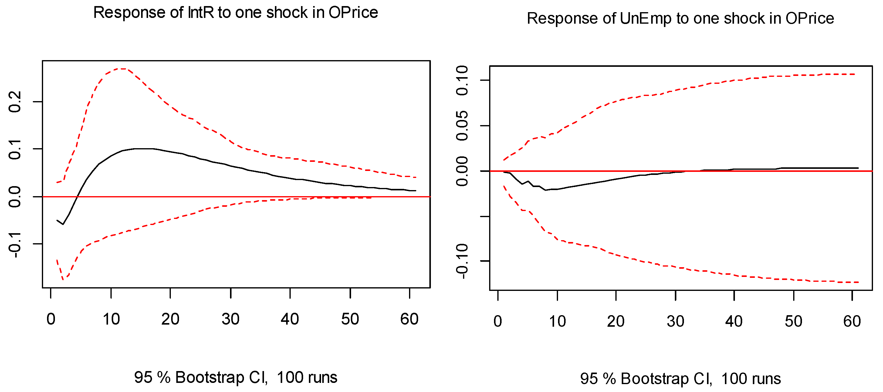
Impulse response analysis was carried out based on the original datasets. To avoid the problem of choosing order of variables in the impulse response function analysis, which contains more than three variables, we first built three bivariate VAR or Vector error correction model (VECM) based separately on interest rate and unemployment, oil price and interest rate, and oil price and unemployment. Then, the impulse response analysis was performed. Unit root and co-integration test results showed that interest rate is stationary while the other two series are co-integrated. Therefore, we built a VAR model to the bivariate combinations of interest rate and unemployment, and oil price and interest rate, while a VECM model was used for the bivariate combination of oil price and unemployment. We did not proceed with impulse response analysis in cases where almost no significant Granger causal relationships were detected at any wavelet scales, namely responses of real oil prices to unemployment and those of real oil prices to interest rates. Therefore, out of the possible six bivariate combinations that can be built for the impulse response functions, we present four of them in Figure 5 and Figure 6. Real interest rate, real oil price, and unemployment are denoted as InR, OPrice and Unemp, respectively, in the following figures. Interpretation of the impulse response functions are done in association with the signs of the response of the investigated causal variable to the investigated caused variable at the lag matching the wavelet scale, for example, the eighth-sixteenth lags for wavelet scale of 8–16 months. We focused on lags at matching wavelet scales where Granger casualty tests showed significant results.
The two graphs in Figure 5 show the responses of interest rate and unemployment to shocks of one standard deviation to the real oil price. In both figures, the confidence interval (the red dashed lines) contains zero; thus, the results were not statistically significant. However, we were still able to form a general impression of how the interest rate and unemployment rate respond to random shocks to oil price. From the sixteenth lag onwards, in the response of interest rate to oil shock (when the Granger causality results showed significant results at the corresponding wavelet scales of 16–32 months), positive signs can be observed, although they are not significant in the impulse response function. We can focus on the same lags of the responses of unemployment to the real oil price. At the lags of sixteen and onwards, the unemployment rate responded negatively to the oil price shock. In association with the Granger causality test above, an increase in oil price decreases unemployment in Norway, a finding that is expected by the theories described in Section 2.1.1. As an oil exporting country, an increase in oil prices does not increase unemployment, which is often the case for the oil importing economies.
The two graphs in Figure 6 above show the impulse responses between interest rate and unemployment. Both impulse responses were significant in certain lags, but not significant in general. Thus, here as well, we concentrated on analysing the sign of the response. For real interest rate responses to unemployment shock, from the fourth lags onwards, significant Granger causal relationships were detected. Unemployment shock decreased interest rate with the maximum effect around one year, and this effect continued for up to around five years, but died off over time. The effect of interest rate on unemployment (with a focus on 8th–16th lags, and 32nd lag and onwards) was negative until around the 10th lag, but became positive from about one year onwards.
5. Conclusions and Policy Implications
This paper investigated the Granger causality among real oil prices, real interest rates, and unemployment in Norway at different time scales by using the wavelet decomposition technique. The empirical framework is based on an efficiency wage model of Carruth et al. [1] and Doğrul and Soytas [4]. In the wavelet decomposition of the current paper, a multiresolution analysis (MRA) for maximal overlap discrete wavelet transform (MODWT) was used to filter the data of interest. Subsequently, the traditional Granger test in VAR framework as well as a relatively new time series technique known as the Toda–Yamamoto procedure (Toda and Yamamoto [36]) are applied for the causality test. Furthermore, impulse responses are also investigated to consider what sign is likely associated with any Granger casualty found.
In general, Granger causality test results showed that causal relationships between the variables grow stronger as the time scale increases. More specifically, no causal relationships, using a 5% significance level, were found among the variables at the smallest time scales of one to three months. The causal relationship from unemployment rate to interest rate was observed from the time scale of two quarters to four quarters. At this time scale, a causal relationship was also found in the opposite direction, creating a feedback relationship between unemployment and interest rate. At the largest scale of eight quarters, causal relationships were evident from oil price to both interest rate and unemployment; furthermore, unemployment Granger causes interest rate. The results of the impulse response functions were often statistically insignificant; however, a general impression could be formed that, in association with Granger causality analysis, unemployment rates in Norway respond negatively to oil price shocks around two years after the shocks occur. As an oil exporting country, increases (or decreases) in oil prices reduce (or increase) unemployment in Norway under a time horizon of about two years; previous studies focused on oil importing economies have generally found the inverse to be true.
Our findings, based on time-varying relationships, have important practical implications for policymakers. First, the effects of the changes in oil price on the labour market are not immediately observable, becoming evident after approximately two years. This dynamic mechanism between oil price and the labour market should thus be incorporated into short-run stabilization policy. Simultaneously, in order for stabilization policy to have its expected effects on the real economy, country-specific responses to oil price changes must be thoroughly investigated before setting policy measures. Second, monetary policy decisions on changes to interest rates should incorporate the effects of oil prices, among others, by accounting for the time horizons within which those effects vary. In essence, policy makers must also realize that the dynamics of unemployment and other relevant factors may differ at different time horizons both in terms of magnitude and signs.
Author Contributions
H.K.K. worked on overall structure of the paper as well as data collection, theoretical frameworks, interpretations of the empirical findings. Y.L. did most of the empirical study part of the paper. G.S. provided advisory comment on earlier versions of the paper.
Funding
Y.L. gratefully acknowledge funding from Finance Market Fund (Finansmarkedsfondet): https://www.forskningsradet.no/prognett-finansmarkedsfondet/Home_page/1232959043546) (Project name: Strategic Risk Adoption in Real Options under Multi-Horizon Regime Switching and Uncertainty. Project number 274569).
Conflicts of Interest
The authors declare no conflicts of interest.
References
- Carruth, A.; Hooker, M.; Oswald, A. Unemployment equilibria and input prices: Theory and evidence from the United States. Rev. Econ. Stat. 1998, 80, 621–628. [Google Scholar] [CrossRef]
- Mork, K.A. Oil and the Macroeconomy when Prices Go Up and Down: An Extension of Hamilton’s Results. J. Polit. Econ. 1989, 97, 740–744. [Google Scholar] [CrossRef]
- Kilian, L. A Comparison of the Effects of Exogenous Oil Supply Shocks on Output and Inflation in the G7 Countries. J. Eur. Econ. Assoc. 2008, 6, 78–121. [Google Scholar] [CrossRef]
- Doğrul, H.G.; Soytas, U. Relationship between oil prices, interest rate, and unemployment: Evidence from an emerging market. Energy Econ. 2010, 32, 1523–1528. [Google Scholar] [CrossRef]
- Rasche, R.H.; Tatom, J.A. Energy price shocks, aggregate supply and monetary policy: The theory and the international evidence. Carnegie Rochester Conf. Ser. Public Policy 1981, 14, 9–93. [Google Scholar] [CrossRef]
- Bruno, M.; Sachs, J. Input Price Shocks and the Slowdown in Economic Growth: The Case of U.K. Manufacturing. Rev. Econ. Stud. 1982, 49, 679–705. [Google Scholar] [CrossRef]
- Jorgenson, D.W. The Role of Energy in Productivity Growth. Energy J. 1984, 5, 11–26. [Google Scholar] [CrossRef]
- Hamilton, J.D. A Neoclassical Model of Unemployment and the Business Cycle. J. Polit. Econ. 1988, 96, 593–617. [Google Scholar] [CrossRef]
- Rotemberg, J.J.; Woodford, M. Imperfect competition and the effects of energy price increases on economic activity. J. Money Credit Bank. 1996, 28, 549–577. [Google Scholar] [CrossRef]
- Shapiro, C.; Stiglitz, J.E. Equilibrium unemployment as a worker discipline device. Am. Econ. Rev. 1984, 74, 433–444. [Google Scholar]
- Blanchard, O. Designing Labor Market Institutions, Central Banking, Analysis, and Economic Policies Book Series, 1st ed.; Jorge, R., Andrea Tokman, R., Norman, L., Klaus, S.-H., Eds.; Labor Markets and Institutions, Central Bank of Chile: Santiago, Chile, 2005; Volume 8, pp. 367–381. [Google Scholar]
- Pindyck, R.S.; Rotemberg, J.J. Dynamic factor demands and the effects of energy price shocks. Am. Econ. Rev. 1983, 73, 1066–1079. [Google Scholar]
- Kim, I.M.; Loungani, A. The role of energy in real business cycle models. J. Monet. Econ. 1992, 29, 173–189. [Google Scholar] [CrossRef]
- Atkeson, A.; Kehoe, P. Putty Clay Capital and Energy; Working Paper No. 4833; National Bureau of Economic Research: Cambridge, MA, USA, 1994. [Google Scholar]
- Burbidge, J.; Harrison, A. Testing for the Effects of Oil-Price Rises Using Vector Autoregression. Int. Econ. Rev. 1984, 25, 459–484. [Google Scholar] [CrossRef]
- Hooker, M. What happened to the oil price-macroeconomy relationship? J. Monet. Econ. 1996, 38, 195–213. [Google Scholar] [CrossRef]
- Lee, K.; Ni, S. On the Dynamic Effects of Oil Price Shocks: A Study Using Industry Level Data. J. Monet. Econ. 2002, 49, 823–852. [Google Scholar] [CrossRef]
- Ferderer, J.P. Oil Price Volatility and the Macroeconomy. J. Macroecon. 1996, 18, 1–16. [Google Scholar] [CrossRef]
- Hamilton, J.D. This is what happened to the oil price-macroeconomy relationship. J. Monet. Econ. 1996, 38, 215–222. [Google Scholar] [CrossRef]
- Hamilton, J.D. Oil and the Macroeconomy since World War II. J. Polit. Econ. 1983, 9, 228–248. [Google Scholar] [CrossRef]
- Gisser, M.; Goodwin, T.H. Crude Oil and the Macroeconomy: Tests of Some Popular Notions. J. Money Credit Bank. 1986, 18, 95–103. [Google Scholar] [CrossRef]
- Loungani, P. Oil Price Shocks and the Dispersion Hypothesis. Rev. Econ. Stat. 1986, 68, 536–539. [Google Scholar] [CrossRef]
- Davis, S.J.; Haltiwanger, J. Sectoral Job Creation and Destruction Response to Oil Price Changes. J. Monet. Econ. 2001, 48, 465–512. [Google Scholar] [CrossRef]
- Keane, M.P.; Prasad, E.S. The Employment and Wage Effects of Oil Price Changes: A Sectoral Analysis. Rev. Econ. Stat. 1996, 78, 389–399. [Google Scholar] [CrossRef]
- Uri, N.D. Crude oil price volatility and unemployment in the United States. Fuel Energy Abstr. 1996, 37, 91. [Google Scholar] [CrossRef]
- Mork, K.; Olsen, O.; Mysen, H. Macroeconomic Responses to Oil Price Increases and Decreases in Seven OECD Countries. Energy J. 1994, 15, 19–36. [Google Scholar]
- Jimenez-Rodriguez, R.; Sanchez, M. Oil price shocks and real GDP growth: Empirical evidence for some OECD countries. Appl. Econ. 2005, 37, 201–228. [Google Scholar] [CrossRef]
- Ramsey, J.B.; Lampart, C. Decomposition of Economic Relationships by Timescale Using Wavelets. Macroecon. Dyn. 1998, 2, 49–71. [Google Scholar]
- Vidakovic, B. Statistical Modelling by Wavelets; Wiley: Hoboken, NJ, USA, 1999. [Google Scholar]
- Percival, D.B.; Walden, A.T. Wavelet Methods for Time Series Analysis; Cambridge University Press: Cambridge, UK, 2006. [Google Scholar]
- Gençay, R.; Selçuk, F.; Whitcher, B. An Introduction to Wavelets and Other Filtering Methods in Finance and Economic; Academic Press: San Diego, CA, USA, 2001. [Google Scholar]
- Li, Y.; Shukur, G. Testing for unit roots in panel data using Wavelet ratio method. Comput. Econ. 2013, 41, 59–69. [Google Scholar] [CrossRef]
- Toda, H.Y.; Yamamoto, T. Statistical inference in vector autoregression with possibly integrated processes. J. Econ. 1995, 66, 225–250. [Google Scholar] [CrossRef]
- Enders, W. Applied Econometric Time Series; Wiley: Hoboken, NJ, USA, 2010. [Google Scholar]
- Haar, A. Zur Theorie der orthogonalen Funktionensysteme. Math. Ann. 1910, 69, 331–371. (In German) [Google Scholar] [CrossRef]
- Percival, D.B.; Sardy, S.; Davison, A.C. Wavestrapping time series: Adaptive Wavelet-based bootstrapping. In Nonlinear and Nonstationary Signal Processing; Fitzgerald, W.J., Smith, R.L., Walden, A.T., Young, P.C., Eds.; Cambridge University Press: Cambridge, UK, 2000; pp. 442–471. [Google Scholar]
Figure 1.
Time plots of the monthly crude oil price, interest, and unemployment of Norway.
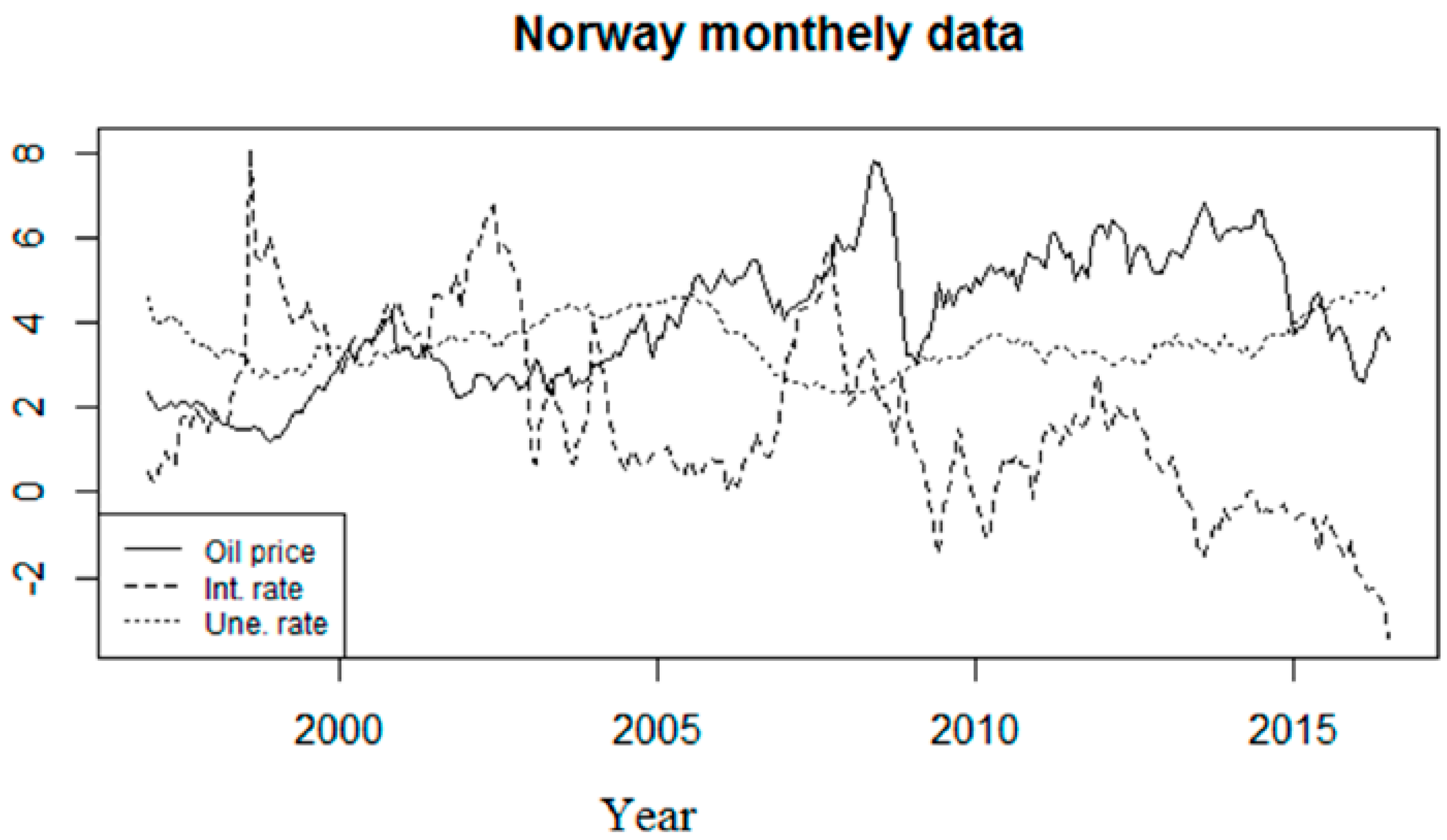
Figure 2.
Time series plot and wavelet decomposition of real oil price (World Texas Intermediate (WTI) Spot Price FOB).
Figure 2.
Time series plot and wavelet decomposition of real oil price (World Texas Intermediate (WTI) Spot Price FOB).
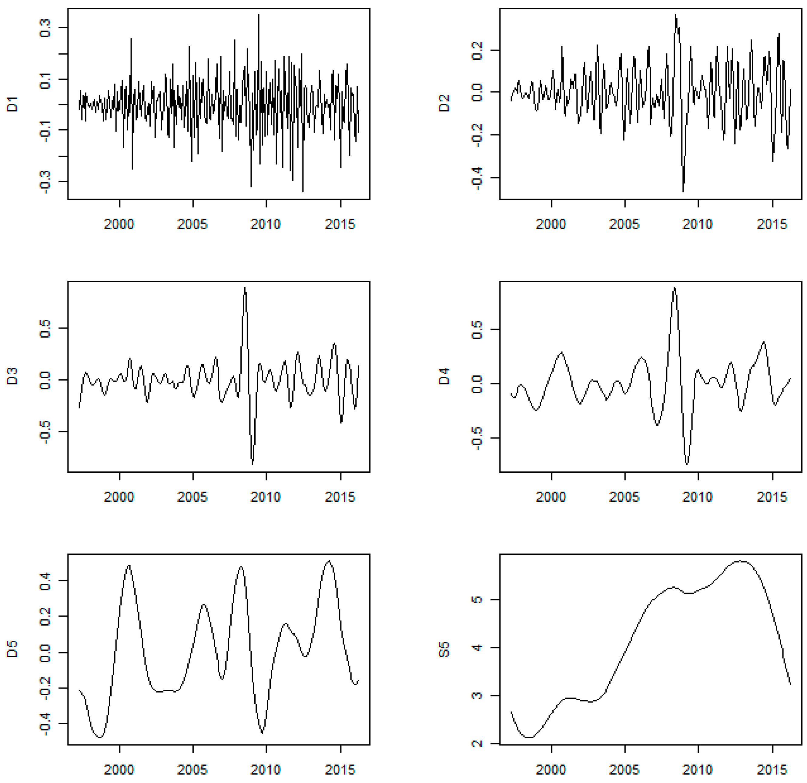
Figure 3.
Time series plot and wavelet decomposition of Norwegian unemployment rate.

Figure 4.
Time series plot and wavelet decomposition of Norwegian real interest rate.
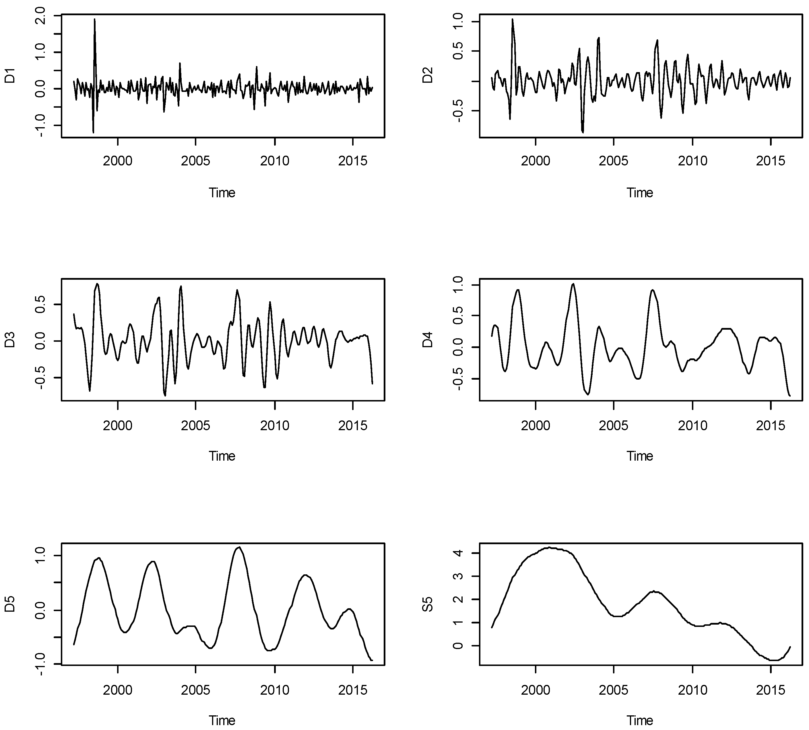
Figure 5.
Impulse responses of interest rate (IntR) and unemployment (Unemp) to oil price (Oprice). CI—confidence interval.
Figure 5.
Impulse responses of interest rate (IntR) and unemployment (Unemp) to oil price (Oprice). CI—confidence interval.

Figure 6.
Impulse responses between the real interest rate (IntR) and unemployment (Unemp).


Table 1.
The p-value table of the Toda–Yamamoto (TY) and Granger causality test for all the scales.
| From | To | S5 * | D5 | D4 | D3 | D2 + D1 |
|---|---|---|---|---|---|---|
| (Interpretations of the Wavelet Scale Notations above) | ||||||
| 32 Months and Longer | 16–32 Month (4–8 Quarter) Cycle | 8–16 Month (2–4 Quarter) Cycle | 4–8 Month (Around Two Quarters) Cycle | 1–3 Month (One Quarter) Cycle | ||
| Oprice | IntR | 0.014 | 0.000 | 0.412 | 0.129 | 0.9566 |
| Oprice | UnEmp | 0.083 | 0.002 | 0.412 | 0.129 | 0.9566 |
| IntR | Oprice | 0.220 | 0.227 | 0.038 | 0.713 | 0.7745 |
| IntR | UnEmp | 0.000 | 0.111 | 0.045 | 0.713 | 0.7745 |
| UnEmp | Oprice | 0.082 | 0.977 | 0.290 | 0.310 | 0.6572 |
| UnEmp | IntR | 0.012 | 0.001 | 0.001 | 0.001 | 0.6572 |
* Toda–Yamamoto procedure was used for testing causality using the smooth series, , because one variable, the real oil price, is not stationary while the others (the real interest rate and unemployment) are stationary. For the detail series, the traditional Granger causality test was used, as all the series are stationary. IntR—real interest rate; Oprice—real oil price; UnEmp—unemployment.
© 2018 by the authors. Licensee MDPI, Basel, Switzerland. This article is an open access article distributed under the terms and conditions of the Creative Commons Attribution (CC BY) license (http://creativecommons.org/licenses/by/4.0/).
Share and Cite
MDPI and ACS Style
Kim Karlsson, H.; Li, Y.; Shukur, G. The Causal Nexus between Oil Prices, Interest Rates, and Unemployment in Norway Using Wavelet Methods. Sustainability 2018, 10, 2792. https://doi.org/10.3390/su10082792
AMA Style
Kim Karlsson H, Li Y, Shukur G. The Causal Nexus between Oil Prices, Interest Rates, and Unemployment in Norway Using Wavelet Methods. Sustainability. 2018; 10(8):2792. https://doi.org/10.3390/su10082792
Chicago/Turabian StyleKim Karlsson, Hyunjoo, Yushu Li, and Ghazi Shukur. 2018. "The Causal Nexus between Oil Prices, Interest Rates, and Unemployment in Norway Using Wavelet Methods" Sustainability 10, no. 8: 2792. https://doi.org/10.3390/su10082792
Note that from the first issue of 2016, this journal uses article numbers instead of page numbers. See further details here.