Quantifying the Role of Large Floods in Riverine Nutrient Loadings Using Linear Regression and Analysis of Covariance

 and
and
Abstract
:1. Introduction
2. Materials and Methods
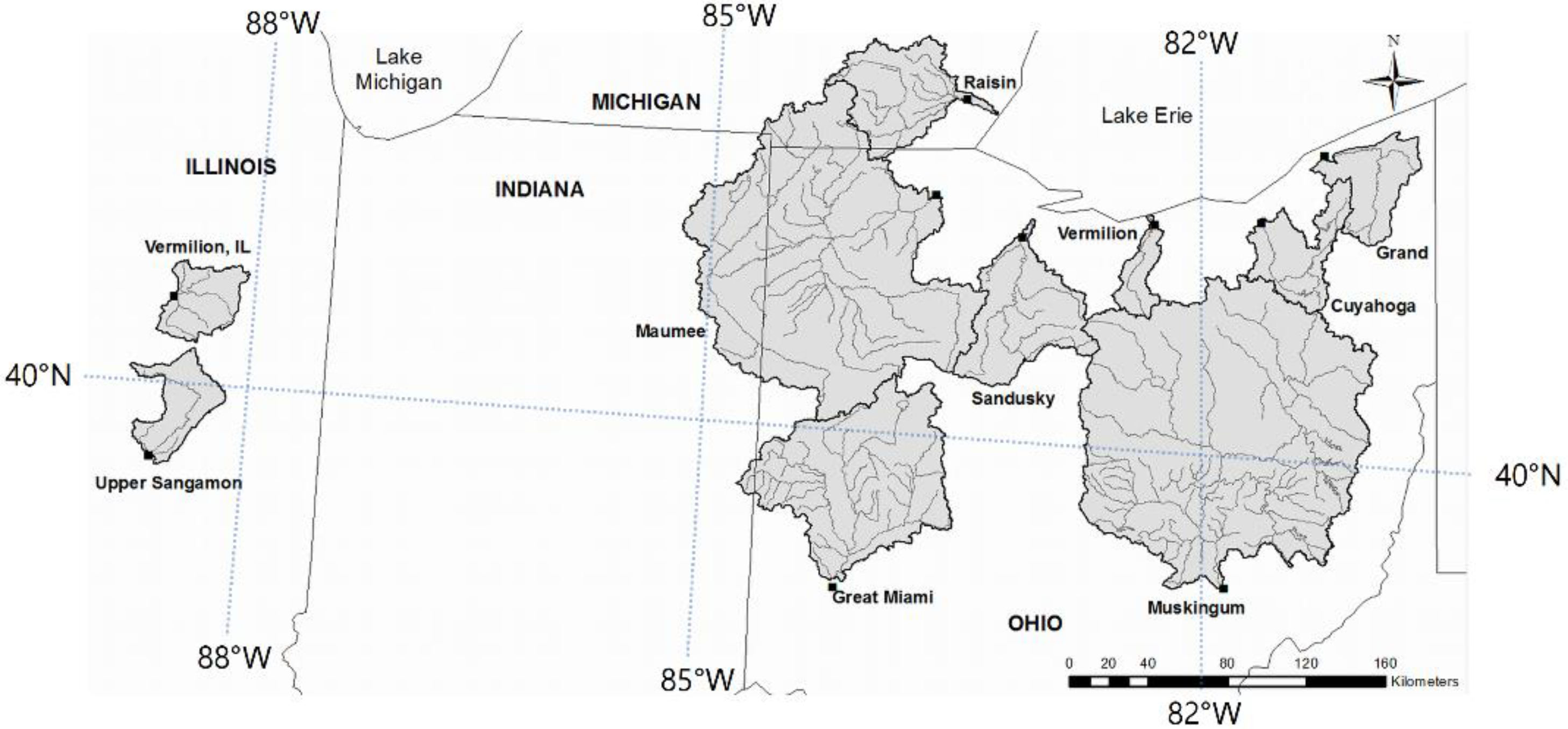
2.1. Site and Data Descriptions
2.2. Separation of Large Events
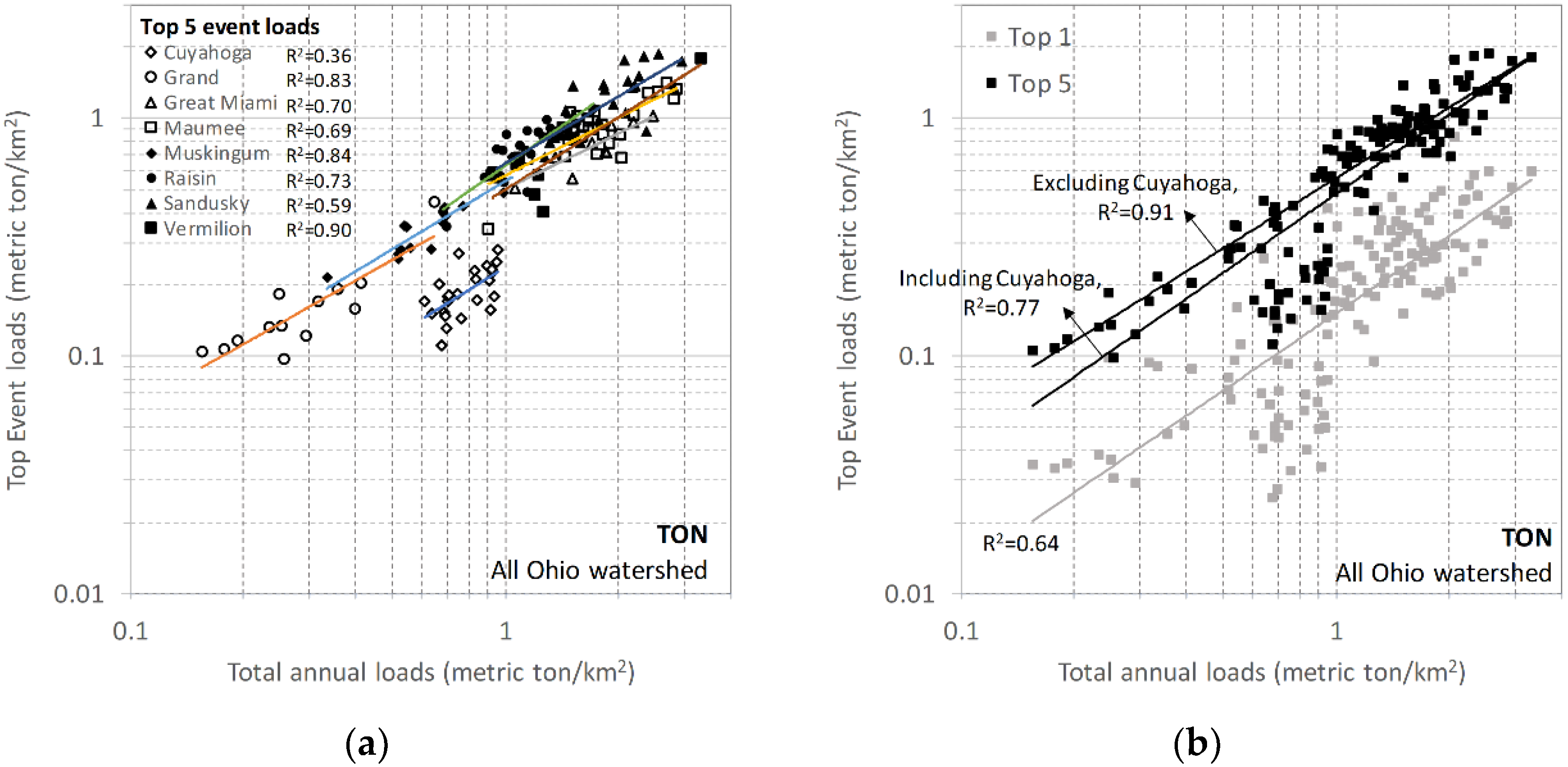
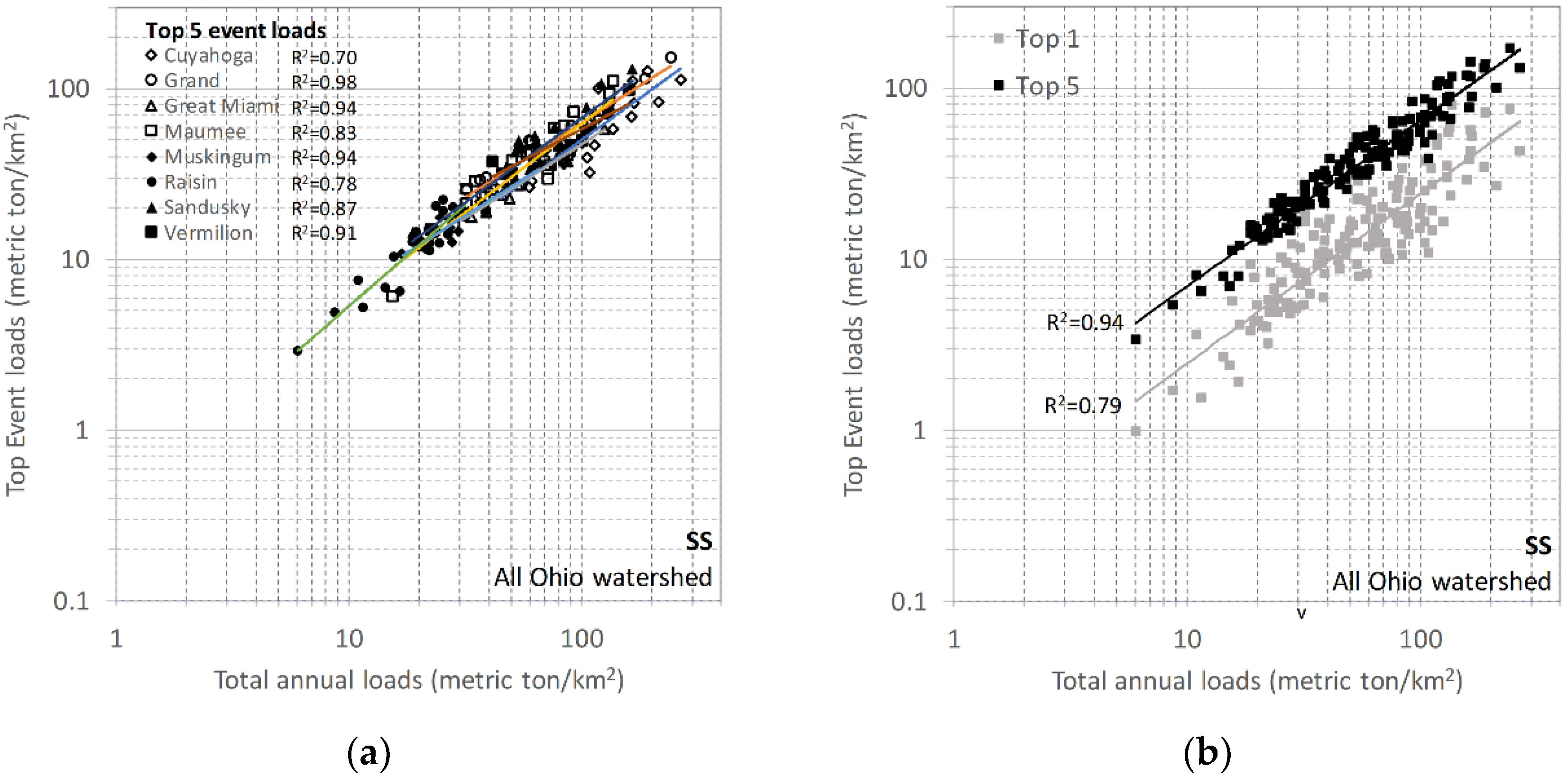
2.3. Predictability of Annual Loads
2.4. Similarity of Predictions
2.5. Applicability of Regression Lines in Other Regions
3. Results
3.1. Large Event Characteristics
3.2. Annual Load Predictions
3.3. ANCOVA
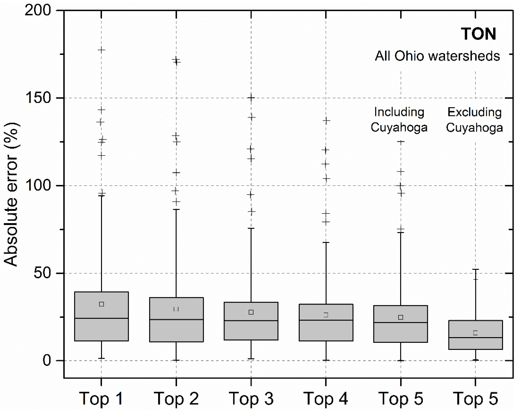
3.4. Error Analysis
3.5. Spatial Transferability
4. Discussion
5. Conclusions
Author Contributions
Funding
Conflicts of Interest
References
- Howarth, R.W. An assessment of human influences on fluxes of nitrogen from the terrestrial landscape to the estuaries and continental shelves of the North Atlantic ocean. Nutr. Cycl. Agroecosyst. 1998, 52, 213–223. [Google Scholar] [CrossRef]
- Kronvang, B.; Jeppesen, E.; Conley, D.J.; Søndergaard, M.; Larsen, S.E.; Ovesen, N.B.; Carstensen, J. Nutrient pressures and ecological responses to nutrient loading reductions in Danish streams, lakes and coastal waters. J. Hydrol. 2005, 304, 274–288. [Google Scholar] [CrossRef]
- Camargo, J.A.; Alonso, Á. Ecological and toxicological effects of inorganic nitrogen pollution in aquatic ecosystems: A global assessment. Environ. Int. 2006, 32, 831–849. [Google Scholar] [CrossRef] [PubMed]
- Goolsby, D.A.; Battaglin, W.A.; Aulenbach, B.T.; Hooper, R.P. Nitrogen input to the Gulf of Mexico. J. Environ. Qual. 2001, 30, 329–336. [Google Scholar] [CrossRef] [PubMed]
- Rabalais, N.N.; Turner, R.E.; Scavia, D. Beyond science into policy: Gulf of Mexico hypoxia and the Mississippi River: Nutrient policy development for the Mississippi river watershed reflects the accumulated scientific evidence that the increase in nitrogen loading is the primary factor in the worsening of hypoxia in the northern Gulf of Mexico. AIBS Bull. 2002, 52, 129–142. [Google Scholar]
- Smith, D.; Livingston, S.; Zuercher, B.; Larose, M.; Heathman, G.; Huang, C. Nutrient losses from row crop agriculture in Indiana. J. Soil Water Conserv. 2008, 63, 396–409. [Google Scholar] [CrossRef]
- Verma, S. Predictability and Trends of Annual Pollutant Loads in Midwestern Watersheds, Dissertation; University of Illinois at Urbana-Champaign: Urbana, IL, USA, 2013. [Google Scholar]
- Yaksich, S.M.; Verhoff, F.H. Sampling strategy for river pollutant transport. J. Environ. Eng. 1983, 109, 219–231. [Google Scholar] [CrossRef]
- Robertson, D.M. Influence of different temporal sampling strategies on estimating total phosphorus and suspended sediment concentration and transport in small streams. JAWRA J. Am. Water Resour. Assoc. 2003, 39, 1281–1308. [Google Scholar] [CrossRef]
- Hirsch, R.M.; Moyer, D.L.; Archfield, S.A. Weighted regressions on time, discharge, and season (WRTDS), with an application to Chesapeake Bay river inputs. JAWRA J. Am. Water Resour. Assoc. 2010, 46, 857–880. [Google Scholar] [CrossRef] [PubMed]
- Natural Resources Conservation Service. National Engineering Handbook, Section 3 Sedimentation; U.S. Department of Agriculture: Washington DC, USA, 1983.
- Smith, R.A.; Schwarz, G.E.; Alexander, R.B. Regional interpretation of water-quality monitoring data. Water Resour. Res. 1997, 33, 2781–2798. [Google Scholar] [CrossRef] [Green Version]
- USEPA. PLOAD Version 3.0: An Arcview GIS Tool to Calculate Nonpoint Sources of Pollution in Watershed and Stormwater Projects; User’s Manual: Washington DC, USA, 2001.
- Tetra Tech Inc. Spreadsheet Tool for the Estimation of Pollutant Load (STEPL); Version 4.0; User’s Guide: Fairfax, VA, USA, 2006. [Google Scholar]
- Richards, R.P.; Holloway, J. Monte Carlo studies of sampling strategies for estimating tributary loads. Water Resour. Res. 1987, 23, 1939–1948. [Google Scholar] [CrossRef]
- Preston, S.D.; Bierman, V.J.; Silliman, S.E. An evaluation of methods for the estimation of tributary mass loads. Water Resour. Res. 1989, 25, 1379–1389. [Google Scholar] [CrossRef]
- Lewis, J. Turbidity-controlled suspended sediment sampling for runoff-event load estimation. Water Resour. Res. 1996, 32, 2299–2310. [Google Scholar] [CrossRef]
- Robertson, D.M.; Roerish, E.D. Influence of various water quality sampling strategies on load estimates for small streams. Water Resour. Res. 1999, 35, 3747–3759. [Google Scholar] [CrossRef] [Green Version]
- Cooper, D.; Watts, C. A comparison of river load estimation techniques: Application to dissolved organic carbon. Environmetrics 2002, 13, 733–750. [Google Scholar] [CrossRef]
- Salles, C.; Tournoud, M.G.; Chu, Y. Estimating nutrient and sediment flood loads in a small Mediterranean river. Hydrol. Process. 2008, 22, 242–253. [Google Scholar] [CrossRef]
- Markus, M.; Demissie, M. Predictability of annual sediment loads based on flood events. J. Hydrol. Eng. 2006, 11, 354–361. [Google Scholar] [CrossRef]
- Lim, K.J.; Engel, B.A.; Tang, Z.; Choi, J.; Kim, K.S.; Muthukrishnan, S.; Tripathy, D. Automated web GIS based hydrograph analysis tool, WHAT. JAWRA J. Am. Water Resour. Assoc. 2005, 41, 1407–1416. [Google Scholar] [CrossRef]
- Baker, D.B. Regional water quality impacts of intensive row-crop agriculture: A lake Erie basin case study. J. Soil Water Conserv. 1985, 40, 125–132. [Google Scholar]
- Richards, R.P.; Baker, D.B. Pesticide concentration patterns in agricultural drainage networks in the lake Erie basin. Environ. Toxicol. Chem. 1993, 12, 13–26. [Google Scholar] [CrossRef]
- Richards, R.P.; Baker, D.B.; Kramer, J.W.; Ewing, D.E.; Merryfield, B.J.; Miller, N.L. Storm discharge, loads, and average concentrations in northwest Ohio rivers, 1975–19951. JAWRA J. Am. Water Resour. Assoc. 2001, 37, 423–438. [Google Scholar] [CrossRef]
- Bosch, N.S.; Allan, J.D.; Dolan, D.M.; Han, H.; Richards, R.P. Application of the soil and water assessment tool for six watersheds of Lake Erie: Model parameterization and calibration. J. Gt. Lakes Res. 2011, 37, 263–271. [Google Scholar] [CrossRef]
- Verma, S.; Markus, M.; Bartosova, A.; Cooke, R.A. Intra-annual variability of riverine nutrient and sediment loadings using weighted circular statistics. J. Environ. Eng. 2018, 144, 04018010. [Google Scholar] [CrossRef]
- Royer, T.V.; David, M.B.; Gentry, L.E. Timing of riverine export of nitrate and phosphorus from agricultural watersheds in Illinois: Implications for reducing nutrient loading to the Mississippi River. Environ. Sci. Technol. 2006, 40, 4126–4131. [Google Scholar] [CrossRef] [PubMed]
- Schilling, K.; Zhang, Y.-K. Baseflow contribution to nitrate-nitrogen export from a large, agricultural watershed, USA. J. Hydrol. 2004, 295, 305–316. [Google Scholar] [CrossRef]
- Zhang, S.; Wang, Z.; Zhang, B.; Song, K.; Liu, D.; Ren, C. Characteristics of Nonpoint Source Pollution from an Agricultural Watershed during Rainfall Events. In Proceedings of the 2010 International Conference on Mechanic Automation and Control Engineering (MACE), Wuhan, China, 26–28 June 2010; pp. 1960–1963. [Google Scholar]
- Zhu, Q.; Schmidt, J.P.; Buda, A.R.; Bryant, R.B.; Folmar, G.J. Nitrogen loss from a mixed land use watershed as influenced by hydrology and seasons. J. Hydrol. 2011, 405, 307–315. [Google Scholar] [CrossRef]
- El-Shaarawi, A.; Kuntz, K.; Sylvestre, A. Estimation of Loading by Numerical Integration. In Developments in Water Science; Elsevier: New York, NY, USA, 1986; Volume 27, pp. 469–478. [Google Scholar]
- Guo, Y.; Markus, M.; Demissie, M. Uncertainty of nitrate-N load computations for agricultural watersheds. Water Resour. Res. 2002, 38. [Google Scholar] [CrossRef]
- Aulenbach, B.T.; Hooper, R.P. The composite method: An improved method for stream-water solute load estimation. Hydrol. Process. 2006, 20, 3029–3047. [Google Scholar] [CrossRef]
- Toor, G.S.; Harmel, R.D.; Haggard, B.E.; Schmidt, G. Evaluation of regression methodology with low-frequency water quality sampling to estimate constituent loads for ephemeral watersheds in Texas. J. Environ. Qual. 2008, 37, 1847–1854. [Google Scholar] [CrossRef] [PubMed]
- Verma, S.; Markus, M.; Cooke, R.A. Development of error correction techniques for nitrate-N load estimation methods. J. Hydrol. 2012, 432, 12–25. [Google Scholar] [CrossRef]
- Troutman, B.M. Errors and parameter estimation in precipitation-runoff modeling: 1. Theory. Water Resour. Res. 1985, 21, 1195–1213. [Google Scholar] [CrossRef]
- Driver, N.E.; Troutman, B.M. Regression models for estimating urban storm-runoff quality and quantity in the United States. J. Hydrol. 1989, 109, 221–236. [Google Scholar] [CrossRef]
- Kočić, A.; Hengl, T.; Horvatić, J. Water nutrient concentrations in channels in relation to occurrence of aquatic plants: A case study in Eastern Croatia. Hydrobiologia 2008, 603, 253–266. [Google Scholar] [CrossRef]
- Snedecor, G.W.; Cochran, W.G. Statistical Methods, 7th ed.; Iowa State University Press: Ames, IA, USA, 1980. [Google Scholar]
- Rozemeijer, J.C.; Van der Velde, Y.; Van Geer, F.C.; De Rooij, G.H.; Torfs, P.J.; Broers, H.P. Improving load estimates for NO3 and P in surface waters by characterizing the concentration response to rainfall events. Environ. Sci. Technol. 2010, 44, 6305–6312. [Google Scholar] [CrossRef] [PubMed]
- Bosch, N.S. The influence of impoundments on riverine nutrient transport: An evaluation using the soil and water assessment tool. J. Hydrol. 2008, 355, 131–147. [Google Scholar] [CrossRef]
- Johnes, P. Uncertainties in annual riverine phosphorus load estimation: Impact of load estimation methodology, sampling frequency, baseflow index and catchment population density. J. Hydrol. 2007, 332, 241–258. [Google Scholar] [CrossRef]
- Mississippi River/Gulf of Mexico Watershed Nutrient Task Force. Gulf Hypoxia Action Plan 2008 for Reducing, Mitigating, and Controlling Hypoxia in the Northern Gulf of Mexico and Improving Water Quality in the Mississippi River Basin; Mississippi River/Gulf of Mexico Watershed Nutrient Task Force: Washington, DC, USA, 2008.
- Lake Erie LaMP. Lake Erie Binational Nutrient Management Strategy: Protecting Lake Erie by Managing Phosphorus; The Lake Erie LaMP Work Group Nutrient Management Task Group: 2011. Available online: https://www.google.com/url?sa=t&rct=j&q=&esrc=s&source=web&cd=2&ved=2ahUKEwix3Lfk4OncAhXU7mEKHaQVDV4QFjABegQICBAC&url=https%3A%2F%2Fwww.epa.gov%2Fsites%2Fproduction%2Ffiles%2F2015-10%2Fdocuments%2Fbinational_nutrient_management.pdf&usg=AOvVaw0AZy3T8q6iS01LiQvILky1 (accessed on 13 August 2018).
- Illinois Agriculture NPS Subcommittee. Draft Notes; Urbana-Champaign Sanitary District: Urbana, IL, USA, 2014.


| USGS Station Number | Monitoring Period | Watershed Size (km2) | Years Selected | Land-Use (%) * | |||
|---|---|---|---|---|---|---|---|
| Agriculture | Urban | Wooded | |||||
| Lake Erie basin | |||||||
| Cuyahoga (Cu) | 04208000 | 1982–2009 | 1843 | 24 | 17 | 47 | 35 |
| Grand (Gr) | 04212100 | 1989–2006 | 1758 | 13 | 37 | 10 | 52 |
| Maumee (Ma) | 04193500 | 1975–2009 | 16,427 | 29 | 81 | 11 | 8 |
| Raisin (Ra) | 04176500 | 1982–2007 | 2755 | 23 | 72 | 11 | 16 |
| Sandusky (Sa) | 04198000 | 1975–2005 | 3285 | 25 | 83 | 9 | 8 |
| Vermilion (Ve) | 04199500 | 2001–2008 | 697 | 7 | 71 | 1 | 26 |
| Ohio River basin | |||||||
| Great Miami (Gm) | 03271601 | 1996–2009 | 6953 | 10 | 82 | 5 | 10 |
| Muskingum (Mu) | 03150000 | 1995–2009 | 19,208 | 14 | 52 | 2 | 43 |
| ANCOVA | Cu | Gr | Gm | Ma | Mu | Ra | Sa | Ve | ALL | |||||||||||||||||||
|---|---|---|---|---|---|---|---|---|---|---|---|---|---|---|---|---|---|---|---|---|---|---|---|---|---|---|---|---|
| R | S | I | R | S | I | R | S | I | R | S | I | R | S | I | R | S | I | R | S | I | R | S | I | R | S | I | ||
| TON | Cu | 0 | 0 | 2 | 0 | 0 | 2 | 0 | 0 | 2 | 0 | 0 | 2 | 0 | 0 | 2 | 0 | 0 | 2 | 0 | 0 | 2 | 2 | 0 | 2 | |||
| Gr | 0 | 0 | 2 | 0 | 0 | 0 | 0 | 0 | 1 | 0 | 0 | 0 | 0 | 0 | 1 | 0 | 0 | 0 | 0 | 0 | 0 | 1 | 0 | 1 | ||||
| Gm | 0 | 0 | 2 | 0 | 0 | 0 | 0 | 0 | 2 | 0 | 0 | 2 | 0 | 0 | 0 | 0 | 0 | 1 | 1 | 0 | 0 | 2 | 0 | 0 | ||||
| Ma | 0 | 0 | 2 | 0 | 0 | 1 | 0 | 0 | 2 | 0 | 0 | 0 | 0 | 0 | 0 | 0 | 0 | 0 | 0 | 0 | 1 | 2 | 0 | 2 | ||||
| Mu | 0 | 0 | 2 | 1 | 0 | 0 | 0 | 0 | 2 | 0 | 0 | 0 | 0 | 0 | 0 | 1 | 0 | 0 | 2 | 0 | 0 | 2 | 0 | 0 | ||||
| Ra | 0 | 0 | 2 | 0 | 0 | 1 | 0 | 0 | 0 | 0 | 0 | 0 | 0 | 0 | 0 | 0 | 0 | 0 | 1 | 0 | 1 | 2 | 0 | 2 | ||||
| Sa | 0 | 0 | 2 | 0 | 0 | 0 | 0 | 0 | 1 | 0 | 0 | 0 | 0 | 0 | 0 | 0 | 0 | 0 | 0 | 0 | 0 | 2 | 0 | 2 | ||||
| Ve | 0 | 0 | 2 | 0 | 0 | 0 | 0 | 0 | 0 | 0 | 0 | 1 | 0 | 0 | 0 | 0 | 0 | 1 | 0 | 0 | 0 | 0 | 0 | 0 | ||||
| ALL | 0 | 0 | 2 | 0 | 0 | 1 | 0 | 0 | 0 | 0 | 0 | 0 | 0 | 0 | 0 | 0 | 0 | 2 | 0 | 0 | 2 | 0 | 0 | 0 | ||||
| TP | Cu | 0 | 0 | 2 | 0 | 0 | 0 | 0 | 0 | 2 | 0 | 0 | 2 | 0 | 0 | 2 | 0 | 0 | 2 | 0 | 0 | 1 | 0 | 0 | 2 | |||
| Gr | 1 | 0 | 0 | 0 | 0 | 0 | 1 | 0 | 2 | 0 | 0 | 1 | 0 | 0 | 2 | 0 | 0 | 2 | 1 | 0 | 0 | 2 | 0 | 1 | ||||
| Gm | 0 | 0 | 2 | 0 | 0 | 0 | 0 | 0 | 2 | 0 | 0 | 2 | 0 | 0 | 0 | 0 | 0 | 0 | 0 | 0 | 0 | 0 | 0 | 0 | ||||
| Ma | 0 | 0 | 2 | 0 | 0 | 0 | 0 | 0 | 2 | 0 | 0 | 2 | 0 | 0 | 0 | 0 | 0 | 0 | 0 | 0 | 0 | 0 | 0 | 0 | ||||
| Mu | 1 | 0 | 2 | 0 | 0 | 1 | 0 | 0 | 1 | 1 | 0 | 2 | 0 | 1 | 0 | 0 | 0 | 1 | 1 | 0 | 0 | 2 | 0 | 0 | ||||
| Ra | 0 | 0 | 2 | 0 | 2 | 0 | 0 | 0 | 2 | 0 | 0 | 0 | 0 | 1 | 0 | 0 | 0 | 0 | 0 | 0 | 0 | 2 | 0 | 1 | ||||
| Sa | 0 | 0 | 2 | 0 | 0 | 2 | 0 | 0 | 2 | 0 | 0 | 0 | 0 | 0 | 1 | 0 | 0 | 0 | 0 | 0 | 1 | 2 | 0 | 2 | ||||
| Ve | 0 | 0 | 1 | 0 | 0 | 0 | 0 | 0 | 0 | 0 | 0 | 0 | 0 | 0 | 0 | 0 | 0 | 0 | 0 | 0 | 1 | 0 | 0 | 0 | ||||
| ALL | 0 | 0 | 2 | 0 | 0 | 0 | 0 | 0 | 1 | 0 | 0 | 0 | 0 | 0 | 0 | 0 | 0 | 1 | 0 | 0 | 2 | 0 | 0 | 0 | ||||
| SS | Cu | 0 | 0 | 2 | 0 | 0 | 0 | 0 | 0 | 0 | 0 | 0 | 0 | 0 | 0 | 1 | 0 | 0 | 2 | 0 | 0 | 0 | 0 | 0 | 2 | |||
| Gr | 1 | 0 | 2 | 0 | 0 | 1 | 1 | 1 | 0 | 0 | 0 | 0 | 0 | 1 | 0 | 0 | 0 | 0 | 0 | 0 | 0 | 1 | 0 | 0 | ||||
| Gm | 1 | 0 | 0 | 0 | 0 | 0 | 2 | 2 | 0 | 0 | 0 | 1 | 0 | 1 | 0 | 0 | 0 | 2 | 0 | 0 | 0 | 1 | 0 | 0 | ||||
| Ma | 0 | 0 | 0 | 0 | 0 | 0 | 0 | 0 | 0 | 0 | 0 | 0 | 0 | 0 | 0 | 0 | 0 | 0 | 0 | 0 | 0 | 0 | 0 | 0 | ||||
| Mu | 1 | 0 | 0 | 0 | 0 | 0 | 0 | 0 | 2 | 2 | 2 | 0 | 0 | 0 | 0 | 0 | 0 | 1 | 0 | 0 | 0 | 1 | 0 | 0 | ||||
| Ra | 0 | 0 | 1 | 0 | 1 | 0 | 0 | 1 | 2 | 2 | 2 | 0 | 0 | 0 | 0 | 0 | 0 | 0 | 0 | 1 | 0 | 0 | 0 | 0 | ||||
| Sa | 0 | 0 | 2 | 0 | 0 | 0 | 0 | 0 | 2 | 2 | 2 | 0 | 0 | 0 | 1 | 0 | 0 | 0 | 0 | 0 | 0 | 0 | 0 | 2 | ||||
| Ve | 0 | 0 | 0 | 0 | 0 | 0 | 0 | 0 | 0 | 0 | 0 | 0 | 0 | 0 | 0 | 0 | 1 | 0 | 0 | 0 | 0 | 0 | 0 | 0 | ||||
| ALL | 0 | 0 | 2 | 0 | 0 | 0 | 0 | 0 | 0 | 0 | 0 | 0 | 0 | 0 | 0 | 0 | 0 | 0 | 0 | 0 | 2 | 0 | 0 | 0 | ||||
© 2018 by the authors. Licensee MDPI, Basel, Switzerland. This article is an open access article distributed under the terms and conditions of the Creative Commons Attribution (CC BY) license (http://creativecommons.org/licenses/by/4.0/).
Share and Cite
Verma, S.; Bartosova, A.; Markus, M.; Cooke, R.; Um, M.-J.; Park, D. Quantifying the Role of Large Floods in Riverine Nutrient Loadings Using Linear Regression and Analysis of Covariance. Sustainability 2018, 10, 2876. https://doi.org/10.3390/su10082876
Verma S, Bartosova A, Markus M, Cooke R, Um M-J, Park D. Quantifying the Role of Large Floods in Riverine Nutrient Loadings Using Linear Regression and Analysis of Covariance. Sustainability. 2018; 10(8):2876. https://doi.org/10.3390/su10082876
Chicago/Turabian StyleVerma, Siddhartha, Alena Bartosova, Momcilo Markus, Richard Cooke, Myoung-Jin Um, and Daeryong Park. 2018. "Quantifying the Role of Large Floods in Riverine Nutrient Loadings Using Linear Regression and Analysis of Covariance" Sustainability 10, no. 8: 2876. https://doi.org/10.3390/su10082876