Sensitivity Analysis in Socio-Ecological Models as a Tool in Environmental Policy for Sustainability

Banos-Gonzalez, Isabel; Martínez-Fernández, Julia; Esteve-Selma, Miguel-Ángel; Esteve-Guirao, Patricia

doi:10.3390/su10082928

Open AccessArticle

Sensitivity Analysis in Socio-Ecological Models as a Tool in Environmental Policy for Sustainability

by

Isabel Banos-Gonzalez

¹,

Julia Martínez-Fernández

^2,*

,

Miguel-Ángel Esteve-Selma

³ and

Patricia Esteve-Guirao

¹

Departamento de Didáctica de las Ciencias Experimentales, University of Murcia, 30100 Espinardo, Spain

²

New Water Culture Foundation/Sustainability Observatory of Murcia Region, University of Murcia, 30100M Espinardo, Spain

³

Department of Ecology and Hydrology, University of Murcia, 30100 Espinardo, Spain

^*

Author to whom correspondence should be addressed.

Sustainability 2018, 10(8), 2928; https://doi.org/10.3390/su10082928

Submission received: 21 July 2018 / Revised: 10 August 2018 / Accepted: 12 August 2018 / Published: 17 August 2018

(This article belongs to the Special Issue Environmental Policy for Sustainability)

Download

Browse Figures

Versions Notes

Abstract

:

The assessment of environmental policies and sustainability in socio-ecological systems (SES) should be tackled from a holistic perspective, using methodologies such as dynamic system models. However, the integral assessment of SES generally suffers from high levels of uncertainty. In this work, the potential of sensitivity analysis (SA) to assess uncertainty and its implications in SES models, specifically in the Fuerteventura sustainability model, has been explored. An extensive SA was applied in different stages of model development and application. The different SA techniques applied allowed, besides a detailed assessment of robustness, the identification of leverage points and their application to define environmental policies and management measures intended to improve sustainability. The results suggest that measures based on leverage points identified by the SA in the model are more effective than others proposed so far by different agents. Furthermore, the assessment of uncertainty of measures thought to contribute to sustainability shows that, when uncertainty ranges are considered, the thresholds of some sustainability indicators might be exceeded, whereas mean values would not. Therefore, the surpassing of some sustainability thresholds might go unnoticed if uncertainties are not considered in the policy analysis. This work shows SA to be a powerful tool that provides important insights to policy makers and end users, with regard to improving environmental policies for sustainability.

Keywords:

leverage point; policy assessment; sustainability indicators; system dynamic models; uncertainty

1. Introduction

1.1. Uncertainty in the Assessment of Sustainability Policies in Socio-Ecological Systems

The assessment of sustainability in socio-ecological systems (SES) should be tackled from a holistic perspective that enables an integral analysis of socioeconomic and ecological factors and their nonlinear interactions and feedbacks [1]. The application of the system dynamic modelling approach has numerous advantages in this assessment, due to its capacity to conceptualize their complex interrelationships and to facilitate their comprehension and monitoring, with the aim of generating useful information for decision-making [2,3].

Nevertheless, the integral assessment of SES generally suffers from high levels of uncertainty [4]. Uncertainty, as has been pointed out [5], represents “an analytical state of limited knowledge which aggravates the exact depiction of a system’s current situation or the future outcomes of the system’s development”. For several authors [6,7], uncertainty analysis is indispensable in modelling since it illuminates the adequacy of models and reveals the reliability of the model outputs. Since policy makers make their decisions based on the available information, the evaluation and minimization of uncertainties, to avoid bias or even faults in decision making, are crucial [5,8]. Policy and scenario analysis might be a tool to deal explicitly with different assumptions about the future, which is inherently uncertain [9].

Moreover, complex socio-ecological models are usually controlled by a high number of parameters, which may constitute a problem in their application and transferability [10]. In addition to the already mentioned purposes of uncertainty analysis, the importance of discovering policy leverage opportunities has been highlighted [11,12]. This refers to regions in parameters space where policy interventions may be particularly efficient and, therefore, useful for decision-making processes [13].

An extensive sensitivity analysis (SA) applied in different stages of model development and application is presented in this paper. This is done with the Fuerteventura sustainability dynamic model (FSM), developed as a tool to assess the expected effects of different environmental policies, intended to achieve a more sustainable development of this insular socio-ecological system [14,15]. The SA was applied to answer the following questions:

(i): Are all the model parameters really required? Is the model as simple as possible?
(ii): How robust are the conclusions derived from the model?
(iii): Which parts of the system have the greatest influence on sustainability outcomes?
(iv): How does uncertainty affect the assessment of environmental policies intended to achieve sustainability?

Thus, the main purpose of this paper is to develop a strategy based on sensitivity analysis to address the following objectives: (i) To improve model formulation, by identifying insensitive parameters which can be removed from the model; (ii) to perform a detailed assessment of model robustness; (iii) to identify the system parameters which have the greatest influence on sustainability, as a basis to define efficient environmental policies; (iv) to explore how uncertainty affects the assessment of different environmental policy options in relation to improved sustainability.

1.2. Case Study: The Fuerteventura Sustainability Dynamic Model (FSM)

1.2.1. Study Area

The arid island of Fuerteventura (The Canary Islands, Spain), with an average annual rainfall below 120 mm, has experienced a later tourism development than the other islands of the archipelago. Nevertheless, tourism has already become the main driving force of the socioeconomic and environmental changes on the island [16]. Due to these recent changes and the vulnerability of its ecosystems, Fuerteventura is considered a relevant case in which the management and decision-making process in relation to a more sustainable development can be analyzed.

The most challenging themes regarding sustainability on the island were identified by an expert panel in the framework of the XI^th Atlantic Conference of the Environment, and they are also found in the Fuerteventura Biosphere Action Plan [17]. Among these challenges, the following are taken into account in this work when policy measures are assessed:

Landscape and high quality natural vegetation degradation [18].
Increasing residential and tourism development. Abandonment of traditional activities [19].
Rising concern about key species conservation [20,21].

1.2.2. Model Description

The building of the Fuerteventura sustainability dynamic model (FSM, [14,15]) arose as a tool to assist decision-makers in the sustainable management of natural resources of the island in the long-term.

The FSM, built by following the system dynamics methodology [22,23], provides in-depth knowledge of the main components of this socio-ecological system and their changes over time. It is structured in five sectors (Socio-tourism, Land Uses, Biodiversity, Environmental Quality and Water Resources), and it includes 520 variables. As part of the model variables, 37 sustainability indicators were integrated into the FSM. Moreover, 110 parameters—constants or coefficients—were identified in the model. Details of the model equations, which link variables and parameters, can be found in References [14,15]. A brief conceptual description of the model is provided below.

Regarding the Socio-tourism sector, tourism represents the main driving force of the employment and wealth generation in Fuerteventura. The migratory flows are strongly influenced by the employment provided by the activities of the tourists. The rising trends in the tourist and resident population have a strong impact on the dynamics of the urban land uptake. Besides, tourism and related activities have substituted traditional productive activities, such as ranching, artisanal fishing, and farming of non-irrigated land in ‘gavias’, a traditional agro-ecosystem [19].
The different land uses and their changes over time are considered in the Land Use sector, which includes three categories: urban uses, agricultural uses and natural areas. Some land use changes result in the degradation of the high quality natural vegetation of the island; this represents one of the main threats to the sustainable development of Fuerteventura, according to the Action Plan of the Biosphere Reserve [17,18].
The Biodiversity sector is focused on two endangered and endemic bird subspecies of the Canary Islands: the Canarian houbara bustard (Chlamydotis undulada fuertaventurae) and the Egyptian vulture (Neophron percnopterus majorensis). Their modelling shows how certain changes which have happened on the island have affected these species in recent decades [20,21,24].
The scarcity of water resources has traditionally represented one of the limiting factors for the development of this arid island. Nevertheless, the advances in seawater desalination have overcome this limitation. The Water Resources sector also includes the groundwater and the surface resources, which are not enough to satisfy the demands of the population or the irrigation requirements. This highlights the importance of the role of desalination in covering the total water demand [14]. Therefore, the island is highly dependent on energy consumption, even to supply a basic need such as the water demand.
The Environmental Quality sector allows the quantification of some indicators regarding the energy generation and consumption, such as the share of renewable energies, and the per capita CO₂ emissions of the island.

1.2.3. Parameters of the Fuerteventura Sustainability Dynamic Model

As aforementioned, the FSM includes 110 parameters, which are part of the different model equations. The values of the parameters were determined directly when data were available (e.g., statistics, local sources and scientific literature), as shown in Table A1. When no reliable information was found, as was the case for 13 parameters, an automatic calibration process was carried out [25], which allowed the selection of the parameter values that maximized the adjustment of the simulation results of the model to the observed data [14]. During this process, the parameter ranges were constrained to realistic levels for the target system, since this increases the power of the calibration without compromising the resulting model structure [26]. All these parameters were subjected to a SA, the purpose of this work, as described in the following sections.

1.2.4. Model Testing

The FSM was calibrated for the 1996–2011 period, by means of a set of model testing procedures [27] including: a dimensional consistency test, an extreme conditions test, a goodness of fit test for the 20 variables with available series of observed data series (See details in Table A2), and a preliminary SA. The model successfully passed the testing procedures [14,15]. However, in order to improve the evaluation of the robustness of the model, its potential regarding the identification of environmental measures to improve sustainability [28], and how uncertainty affects the assessment of the sustainability of specific measures, a deeper SA was carried out in this work.

2. Methodology

2.1. Sensitivity Analysis

Different SA techniques were applied, ranging from a local sensitivity analysis, using the simplest class of “One factor at a time” screening techniques (OAT), to general sensitivity techniques, such as Monte Carlo simulation. The purpose was not to select one of the two methods but to benefit from their complementarities, regarding the objectives set out in Section 1.1.

2.1.1. Objective 1: To Improve Model Formulation, by Removing the Less Sensitive Parameters

One factor at a time (OAT) sensitivity analysis allows for the identification of those parameters to which the behavior of the model is not responsive. Then, the model structure can be simplified, removing those parameters and achieving a more compact model without losing information valuable for the system [29].

Moreover, for the FSM, a complex model with more than 500 variables and parameters and long computational run times, the OAT was used prior to a general SA [28]. In spite of its shortcomings—since it does not take into account interactions resulting from the simultaneous variation of multiple parameters—the OAT method has its strengths (easy and rapid evaluation of the effects of extreme parameter values) and has been widely applied [30,31]. Furthermore, the general sensitivity techniques applied later allow the mentioned drawbacks to be overcome [32].

In this work, 18 target variables were selected, by means of which the behavior of the model was assessed. This selection was performed in the framework of the XIth Atlantic Conference of the Environment, due to its representation of the main socio-ecological processes; some of these variables are also sustainability indicators. The screening of the most and least sensitive parameters within the model was undertaken using the OAT sensitivity analysis function within Vensim [33] and a sample size of 200 runs. The response to each one of the model parameters examined was tested using an arbitrarily selected range of ±25% variation around the default parameter value. Some authors [34,35] used ±20% and indicated to other possibilities, such as ±50%. Thus, the effect of each parameter on the model outputs may be compared based on a homogeneous range of variation. The sensitivity index (Si,j; Equation (1), [36]) was calculated for years 2012 and 2025 as follows:

S_{i, j} = (\frac{O M_{i, t} - O m_{i, t}}{O b_{i, t}}) \div (\frac{P M_{j} - P m_{j}}{P b_{j}}) \times 100

(1)

where Si,j represents the sensitivity index of the target variable i in relation to the parameter j; OMi,t and Omi,t are the maximum and minimum values, respectively, of the ith target variable at time t; Obi,t represents the base (default) model value of the ith target variable at time t; PMj and Pmj represent the maximum and minimum values of the jth parameter, respectively; and Pbj is the base model value of the jth parameter.

Regarding this sensitivity index, the parameters will be classified into five categories: insensitive (Si,j = 0%), low sensitivity (Si,j < 10%), moderate sensitivity (10% ≤ Si,j < 50%), high sensitivity (50% ≤ Si,j < 100%), and very high sensitivity (Si,j ≥ 100%).

2.1.2. Objective 2: To Assess the Robustness of the Model Outputs

In order to achieve realistic SA results and avoid running the model under impossible conditions, a screening was carried out using a new local SA. This time, each parameter was perturbed within an “acceptable” or reasonable range [26,34]. This range may have a slightly different meaning: (i) the range in which it is expected to find the true value of the parameter; (ii) the range of real variability of the parameter in the system (observed or predicted variability); and (iii) the realistic values that a parameter might adopt for a certain management measure.

The local SA with acceptable ranges allowed the identification and selection of the most sensitive parameters (Si,j ≥ 50%) for each of the 18 target model variables. These acceptable ranges are important for the general SA, since they ensure that the parameters are constrained to realistic levels and will produce behavior consistent with known facts [37].

Once the sensitive parameters for each target variable had been identified, a Monte Carlo (MC) simulation was carried out, with a Latin Hypercube sampling [38]. This general SA was implemented to assess the effects of a simultaneous variation of all sensitive parameters for each variable. The MC simulation is appropriate when models may generate interactions between factors or have non-linear outputs [39]. A Latin Hypercube search (LH) was applied as a mechanism to ensure that the full reasonable range of each parameter was explored using a manageable number of runs (200 simulations). The LH is designed to reduce the required number of model runs needed to get sufficient information about the distribution in the outcome [35]. This is desirable for big models where each simulation takes a long time, such as the FSM.

In order to obtain the confidence intervals of the model outputs in relation to changes in the most responsive parameters, 18 MC simulations were run (one per target variable). Here, the Vensim tool for the MC simulation was used [33], which provides the 50%, 75%, 95% and 100% percentile bounds of the established simulations run (200 in our case). According to Reference [35], such percentiles can be interpreted, approximately, as the corresponding confidence bounds.

The variation coefficient (VC_i,t, Equation (2)) of the target model variables shown by the MC simulation was calculated for years 2012 and 2025 as follows:

V C_{i, t} = (\frac{O M 95_{i, t} - O m 95_{i, t}}{\bar{O_{i}}}) \times 100

(2)

where VC_i,t represents the relative variation of the target variable i with respect to its mean value using 95% confidence bounds; OM95_i,t and Om95_i,t are the maximum and minimum values of the ith target variable at time t, using the 95% confidence bound; and

\bar{O_{i}}

is the mean value of the target variable i.

Regarding this variation coefficient, the responses of the target model to changes in the most responsive parameters were classified into three categories: low response (VCi < 50%), moderate response (50% ≤ VCi < 100%) and high response (VCi ≥ 100%).

2.1.3. Objective 3: To Identify the Places in the System which have the Greatest Influence, as a Basis to Define Policies for Improving Sustainability

The most responsive parameters from the OAT analysis may be useful in establishing future priorities [40]. In complex socio-ecological systems, it is often possible to find leverage points, defined as “places within a complex system where a small shift in one thing can produce big changes in everything” [41].

In this work, the identification of leverage points was used as the basis to define potential policy options.

2.1.4. Objective 4: To Explore how Uncertainty Affects the Assessment of Different Environmental Policies Intended to Achieve Sustainability

Indicators could represent useful tools to compare the impacts of the alternative options [42,43]. This work shows how a selection of seven indicators (Table 1) would react to different policy measures. These indicators were selected on the basis of their direct relationship with the policies concerned (see Table A3 for their model formulation).

The establishment of thresholds for each indicator is a clear step forward in sustainability since they represent a reference for decisions and quantify what is acceptable regarding sustainability goals [43]. When there were no published thresholds for an indicator, a value was established based on a proportion of the value adopted for that indicator in 2009, when Fuerteventura was declared a Biosphere Reserve [44]. In this work, the value used was 75% of the 2009 value. This is related to the concept of “Limit of Acceptable Change” (LAC) [15,45], since this proportion allows certain change due to socio-touristic development, but the threshold is still far from compromising the conservation goals.

The simulation results obtained with MC analysis for each indicator over the 2012–2025 period, will determine whether the sustainability thresholds of the seven indicators selected might be exceeded under any of the options analyzed when uncertainty is taken into account.

3. Sensitivity Analysis Results

3.1. Improvement of Model Formulation

According to the values of the sensitivity index, 54 of the 110 parameters studied had sensitivity below 10% for all the target model variables, which may be considered as low sensitivity. Moreover, seven of them were removed from the model structure, since they were not sensitive (S_i,j = 0% for all target variables). See Appendix A and Electronic Supplementary Material for details.

After the removal of these insensitive parameters, a new goodness of fit test for the 20 variables, in relation to the available series of observed data series was carried out (see Table A2), to confirm that the goodness of fit had not changed.

3.2. Detailed Assessment of Model Robustness

After the removal of these seven insensitive parameters from the model structure, a new local SA was carried out, varying each parameter within its acceptable range (see Table A1 and Electronic Supplementary Material for details). Therefore, there were now 48 low-sensitivity parameters (S_i,j < 10%), 28 moderate-sensitivity parameters (10% ≤ S_i,j < 50%), and 26 high-sensitivity parameters (S_i,j ≥ 50%). Of these latter parameters, 18 showed high sensitivity for just one target variable; therefore, their impact on the model response was very local. In contrast, five of these high-sensitivity parameters were considered the most responsive: B and BIRBASE (involved in the effect of the Gross Domestic Product on population growth, specifically on births), MFACTOR IET (involved in the computation of the attractiveness to tourists), NGP (grazing proportion), and THRESHOLD OR (occupancy rate of accommodation facilities). Each one of these five parameters is highly sensitive for five or more target variables.

The results of the global SA (Monte Carlo simulations) are shown in Table 2, which also presents the set of sensitive parameters (S_i,j ≥ 50%) for each target variable. The results show a moderate response of the model to changes in parameter values. Half of the 18 variables analyzed showed a low response (variation coefficient below 50%); seven showed a moderate response (variation coefficient between 50% and 100%); and two variables showed a high response (variation coefficient above 100%), which were: the per capita emissions of CO₂ and recycled waste.

Figure 1 shows the results of the Monte Carlo SA simulations. The red, green, blue and yellow areas account for the confidence bounds of 50%, 75%, 95% and 100% of the Monte Carlo simulations, respectively.

3.3. Which Parts of the System Have the Greatest Influence on Sustainability Outcomes?

This section is based on the most responsive parameters from the local SA. This analysis was used to identify the leverage points in the FSM, where decisions can most effectively influence the performance of the system.

As mentioned in Section 3.2, the most responsive parameters were: B, BIRBASE, MFACTOR IET, THRESHOLD OR and NGP. Since the first three parameters came from automatic calibration, the potential of using the latter two parameters to develop effective environmental policy measures was assessed: THRESHOLD OR is related to socio-tourism measures and NGP to the conservation of natural vegetation.

Regarding the socio-tourism dynamics, it was intended to assess a policy aimed at controlling the effect of the tourism on some key variables: resident population, equivalent tourist population and accommodation capacity, in order to moderate the present trend towards high urban and tourism growth in Fuerteventura. Two measures aimed at achieving a more sustainable state were assessed: one based on policies proposed so far (M1), and another based on one of the model leverage points (M2).

Measure 1 (M1). The limitation of new tourist accommodations is modified by changing the maximum number of tourist beds. The maximum tourist accommodation capacity, determined as the MAXACCOMMODATION parameter (Table A1), would be reduced by 10%, in line with the proposal of the General Regulation Directives and the Canary Islands Tourism Regulation Directives—TRD, henceforth [48].

Measure 2 (M2). The limitation of new tourist accommodations is modified by changing the occupancy rate threshold. The development of new tourist accommodation beds is partially determined by the occupancy rate, THRESHOLD OR. The Sensitivity Analysis identified this parameter as a leverage point. In this measure, this parameter is increased by 10%, meaning that the accommodation facilities should maintain a higher occupancy rate before new infrastructure is built-up.

The simulation results (Figure 2) show that a 10% change in MAXACCOMODATION, would mean changes of 4.8%, 1.4% and 4.4% change in the resident population, equivalent tourist population and tourist accommodation, respectively, in 2025; whereas, a 10% change in THRESHOLD OR would mean changes of 24.5%, 22.4% and 29.4%, respectively, in these variables.

Regarding the land use dynamics, the idea was to assess a policy aimed at improving some indicators: the high quality vegetation proportion (hqp), the overgrazing indicator (oi) and the landscape indicator (li). These three indicators would improve if grazing pressure were reduced. To achieve this, two measures were assessed:

Measure 3. The reduction of grazing pressure on high-quality natural vegetation is achieved by restoring the ‘gavias’, the traditional farming system of non-irrigated lands. This measure, supported by the Abandoned Gavias Restoration Plan [49], was tested by increasing the reuse of urban reclaimed water (REUSR) by 10%, to restore abandoned ‘gavias’ and to cultivate in them the fodder for cattle feeding, thereby reducing the needs for grazing on natural vegetation.

Measure 4. Direct reduction of grazing pressure. This measure considers a 10% reduction in the proportion of grazing on the island (NGP). The parameter NGP was identified as a leverage point.

In this case, the simulation results (Figure 3) show that a 10% change in REUSR, would mean changes of around 3.8%, 6.3% and 3.7% change in hqp, oi and li, respectively, in 2025; whereas, a 10% change in NGP would mean changes of 6%, 10% and 5.5% change in these indicators, respectively.

3.4. How Does Uncertainty Affect the Assessment of Environmental Policies Intended to Achieve Sustainability?

Based on the aforementioned measures defined according to the identified leverage parameters and on the main challenges for sustainability in Fuerteventura (Section 1.2), two environmental policies were defined:

Environmental Policy I. Limitation of new tourist accommodations. This policy requires an increase in the occupancy ratio to 75% in the existing accommodation before the building of new tourist facilities, in line with Reference [46]. It might be implemented by different measures, such as a tax on the accommodation capacity.

Environmental Policy II. Reduction of grazing to protect the soil and the high quality natural vegetation. This measure considers a reduction in the net grazing proportion from 50%, under the Business as Usual scenario (BAU), to 29%, as in the case of the neighboring island of Tenerife [50].

To explore how uncertainty affects the assessment of such policies, a set of sustainability indicators and their thresholds were used (Table 1). Table 3 shows the mean value of the MC simulation for each indicator and the 95% confidence bounds for BAU and for the two environmental policies.

The ratio of tourists to locals (tures) would exceed its sustainability threshold under BAU in 2025, both for the mean value and its associated uncertainty with the 95% confidence bound is considered. Under Policy I, this indicator would worsen by around 29% (Table 3).

The same pattern was shown by the ratio of tourist accommodation to the resident population (ear), with a worsening of around 20% under Policy I. The mean values of the simulation results of ear would be far below the threshold under both simulations (BAU and Policy I). Nevertheless, when uncertainty is taken into account, this sustainability threshold might be exceeded.

The percentage of artificial land (alp) would be reduced by almost half under Policy I, with respect to BAU, since the reduction of the tourist and resident populations would slow down the land uptake processes. Fuerteventura would still be far from the sustainability threshold for this indicator, even considering the uncertainty range.

The reduction of land uptake under Policy I would lead to an improvement in the high quality vegetation proportion (hqp) and the houbara habitat proportion (hhp). For the former, hqp, both mean values (BAU and Policy I) would not exceed the threshold, although they might when uncertainty is considered. The threshold of hhp would be exceeded under BAU, but this indicator would remain far from its threshold under Policy I, even when taking its uncertainty into account.

The proportion of Egyptian vultures (Evp) would not exceed its threshold under BAU or Policy I, even when considering its uncertainty. Moreover, this indicator would slightly improve (around 2%) under Policy I.

Regarding Policy II, the hqp would double in value relative to BAU. According to its mean values, this indicator would be far from its threshold, under both BAU and Policy II. However, when uncertainty is taken into account this threshold might be exceeded under BAU, but not under Policy II.

The overgrazing indicator (oi) also would show an improvement, of around 27%, under Policy II. In neither case (BAU or Policy II) would the threshold be exceeded, even taking the uncertainty into account. On the contrary, the reduction in the grazing proportion considered under Policy II would lead to a decrease of 33% in Evp, exceeding its threshold, since for the grazing cattle this constitutes the basis of their diet, whereas the value of this indicator would increase between 2012 and 2025 under BAU.

In summary, under BAU, the mean values of two out of seven indicators (tures and hhp) would exceed their thresholds; but when uncertainty is taken into account, the thresholds of four of the seven indicators might be exceeded. Regarding Policy I, the mean value of one of the seven indicators (tures) would exceed its threshold; but, when uncertainty is considered, the thresholds of three of the seven indicators might be exceeded. Under Policy II, the mean values of three of the seven indicators (tures, hhp, and Evp) would exceed their thresholds; but, when uncertainty is taken into account, the thresholds of four of the seven indicators might be exceeded.

4. Discussion

The Discussion Will Address the Questions Underlined in the Introduction.

4.1. Was the FSM Built as Parsimoniously as Possible?

Parsimony (maximization of the explanatory capacity while keeping a model as simple as possible) is an important attribute in environmental modelling. Hence, the number of parameters should be kept to the minimum number which achieves the best model performance. An important aim of the parameter SA is to allow a reduction in the number of parameters that must be estimated, thereby reducing the computational time required for model calibration [51].

Of the 110 parameters studied, eight were removed from the model structure, since they were not sensitive (S_i,j = 0% for all target variables). This resulted in a more compact and parsimonious model without losing valuable information. The results of a new goodness of fit analysis (Table A2) confirm that, without these parameters, there was no loss of model performance.

4.2. How Robust are the Conclusions Derived from the FSM? May They be Taken into Account in the Decision-Making Process with a Sufficient Level of Confidence?

Decision-makers are increasingly interested in understanding the uncertainties of the models. It has been underlined previously that only by evaluating the nature and extent of the uncertainties in the system can a model provide decision-makers with a realistic picture of the possible outcomes, since it is impossible to predict with certainty the result of each management decision [23,28].

Sensitivity analysis is a critical tool in the evaluation of the reliability of model outputs [38]. The results of the detailed assessment of robustness (Section 3.2) showed that there is sufficient confidence in the model outcomes. In summary, 76% of the parameters showed low to moderate sensitivity, according to the local sensitivity analysis, whereas 16 of the 18 model target variables had low to moderate variation, according to the Monte Carlo analysis.

In particular, the results of the local SA show that the model displays, generally, low to moderate sensitivity to changes in the values of the parameters. The model displays high sensitivity (S_i,j ≥ 50%) for 26 parameters, 24% of the total, while 10 parameters display sensitivity above 100%, meaning that the model interactions might exacerbate the input variation for such parameters [52]. However, for the majority of these high-sensitivity parameters, only one target variable showed a high response. Only five parameters exhibited high sensitivity for five or more target variables; four of these (B, BIRBASE, MFACTOR IET, and THRESHOLD OR) belong to the socio-tourism sector. This is consistent with the findings of several authors [53,54] who stated that tourism is highly influenced by external drivers—including economic, environmental, political, social, technological, and even attitudinal dimensions—which provide a high degree of uncertainty.

At high levels of model complexity, individual sources of uncertainty are more likely to exhibit interactions that may greatly increase the overall model uncertainty. Therefore, in models with many interactions among sources of uncertainty, the overall uncertainty may be amplified [52]. In the FSM, the MC simulation results show that two of the 18 target variables would change markedly (variation greater than 100% with respect to the mean value with its 95% confidence bound) if one were to use their respective combination of most responsive parameters (Table 2). These MC results mean that decision-makers should treat with caution the policy options and measures involving variables with high uncertainty. In Fuerteventura, this is particularly the case for the per capita CO₂ emissions and the recycled waste.

According to Reference [28], as decisions should be made based on the prevailing knowledge, but also acknowledging the gaps in it, transparent representation of uncertainty is recommendable at each level of modelling and stage of decision-making. Moreover, uncertainty should be considered a normal component of decisions and, instead of inaction, it should appeal to the prudence of policy makers [13]. The precautionary principle should be applied in relation to the uncertainty analysis: The higher the uncertainty, the less risky the policy should be [15].

4.3. Which Parts of the System have the Greatest Influence on Sustainability Outcomes?

The identification of the leverage points in the FSM, the most responsive parameters from the local sensitivity analysis, may be useful to establish future priorities and thus to develop the policies that most effectively influence the performance of the system [55,56].

In this work, the potential of using leverage points to develop more effective measures is shown. Leverage points-based measures have been compared with other measures with a similar aim proposed by different agents, by means of two simple cases. The simulation results (Figure 2) show that bigger changes in key socio-ecological variables were achieved under Measure 2 (a 10% change in the occupancy rate threshold, a leverage point), than under Measure 1 (a 10% change in the maximum number of beds, based on the Tourism Regulation Directives (TRD), [48]). These results are consistent with those of other authors [16,57,58] who suggested that the moratorium set out by the TRD has been shown to be insufficient to stop the increase in the number of beds and the impacts it involves.

Regarding policies aimed at improving some indicators related to the conservation of the vegetation, the simulation results (Figure 3) also showed bigger changes in these indicators under Measure 4 (a 10% of reduction in the net grazing proportion, a leverage point), than under Measure 3 (a 10% of change in the water reuse ratio, based on the Abandoned Gavias Restoration Plan, [49]).

These results show that measures based on the identified leverage points have a higher impact than others, including many of those proposed by different agents. This analysis may help decision-makers to reconsider misconceived plans and policies, and thus to direct the political and economic efforts towards more effective environmental measures that improve the overall sustainability of the socio-ecological system concerned.

4.4. How does Uncertainty in Model Outcomes Affect the Assessment of Policies?

It is widely acknowledged that uncertainty needs to be accounted for in impact studies for decision support. Scenario and policy analysis represents a tool to deal explicitly with different assumptions about the future [8]. However, the existing models are often deterministic, without any indication of the amount of uncertainty or expected variation around the simulation values [9]. Some authors highlighted that models which include the uncertainties involving the management options considered may be of considerable added value for the decision-makers [28].

This work has assessed how a set of sustainability indicators included in the model would react under two environmental policy measures based on the identified leverage points. The focus is not only the mean values of these indicators, but also their associated uncertainty ranges.

Regarding Policy I, the limitation of new tourist accommodations would lead to the improvement of two key sustainability indicators, when compared to BAU: the artificial land proportion (alp) and the houbara habitat proportion (hhp). Even when uncertainty is considered, the sustainability thresholds for alp and hhp would not be exceeded under Policy I. In contrast, the ratio of tourists to residents (tures) and the ratio of tourist accommodation to residents (ear) would increase relative to BAU (Table 3), the threshold of tures being exceeded in all the simulations considered. This can be explained by the increase in the resident population, the denominator in both indicators, which would be greater under BAU than under Policy I. This illustrates how possible misunderstandings may appear when relative sustainability indicators (for example, efficiency indicators and per unit indicators, such as per capita or per hectare) are considered alone. Therefore, relative indicators should be viewed with caution to avoid errors in the diagnosis of sustainability [15,59].

Regarding Policy II, the high quality vegetation proportion (hqp) and the overgrazing indicator (oi) would improve. In the case of hqp, this improvement would distance the indicator from its threshold, even when considering its uncertainty. In contrast, the Egyptian vulture population proportion (Evp) would decrease under Policy II, exceeding its threshold. The provision of an estimate of the uncertainty, along with each model outcome, is of crucial importance, since it has the potential to change the management recommendations that are based on the model [28]. In this sense, the surpassing of some sustainability thresholds may have gone unnoticed in previous work when only the mean values of the simulations were considered. As aforementioned, the number of indicators which might exceed their threshold when uncertainty is taken into account would increase from two to four under BAU, from one to three under Policy I, and from three to four under Policy II. These policies are, a priori, thought to be environmentally sound, and Policy I does reduce the number of indicators exceeding their thresholds when the mean values are considered. However, when uncertainty is taken into account, an important finding arises: BAU and both environmental policies are riskier than expected, since the number of indicators exceeding their thresholds is higher.

The work presented here has some shortcomings. Three of the five parameters with high sensitivity were determined by an automatic calibration process, since no other information was available. There is also a lack of knowledge about the acceptable range of change for several of the parameters. Such knowledge would provide greater certainty in the model outputs. These shortcomings will be addressed in subsequent work, which must involve stakeholders and decision-makers for a joint assessment of the results obtained regarding policy measures and their uncertainty.

5. Conclusions

In this paper, a set of analyses has been applied to a socio-ecological model, the Fuerteventura sustainability dynamic model (FSM), in order to improve the model as a tool for management and the decision-making process. These analyses have allowed:

The improvement of the model formulation by removal of the least sensitive parameters, by means of screening techniques such as one factor at a time (OAT). Eight insensitive parameters were removed, making the model more compact and parsimonious.
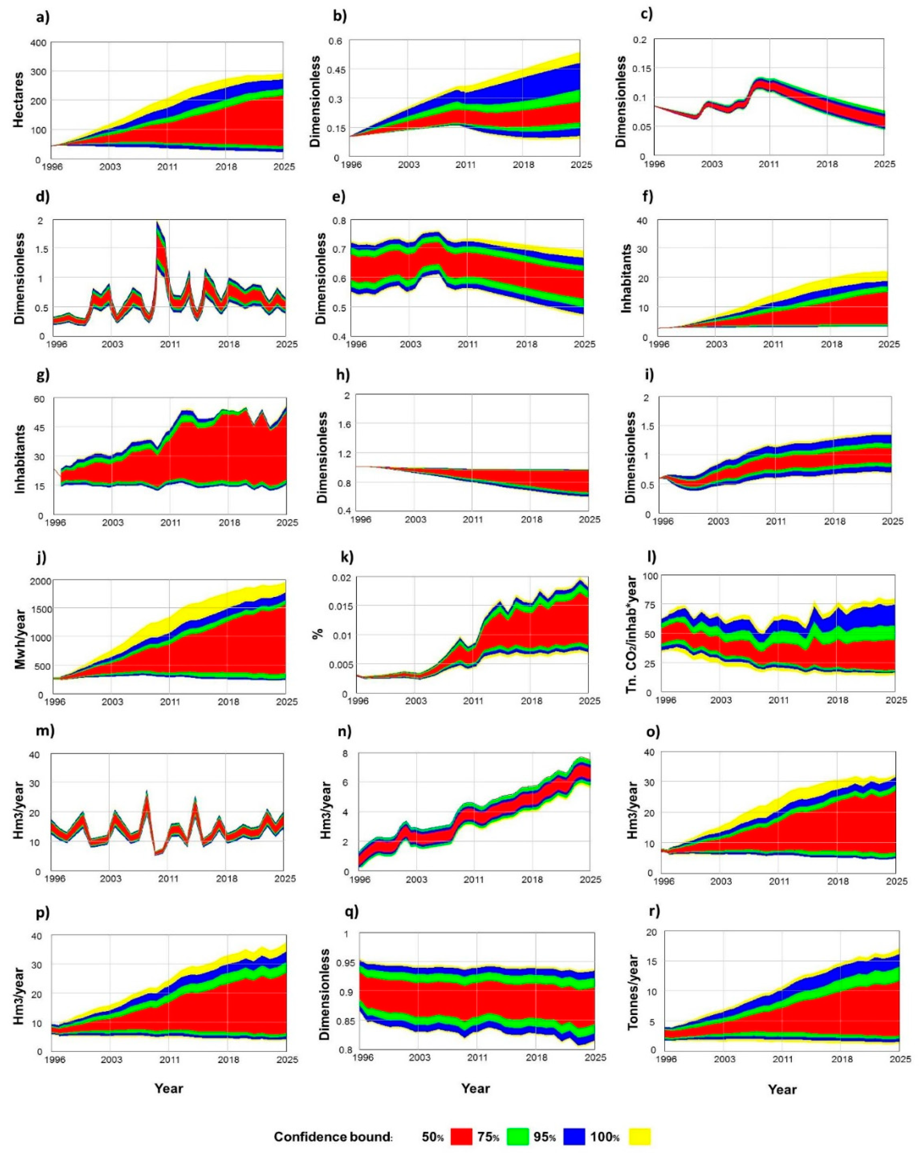
A detailed assessment of robustness. The Monte Carlo simulations showed a low (variation lower than 50% with respect to the mean value) to moderate (variation between 50% and 100%) response for 16 of the 18 target model variables to changes in the values of their most responsive parameters, which means that the model outcomes can be accepted with confidence.
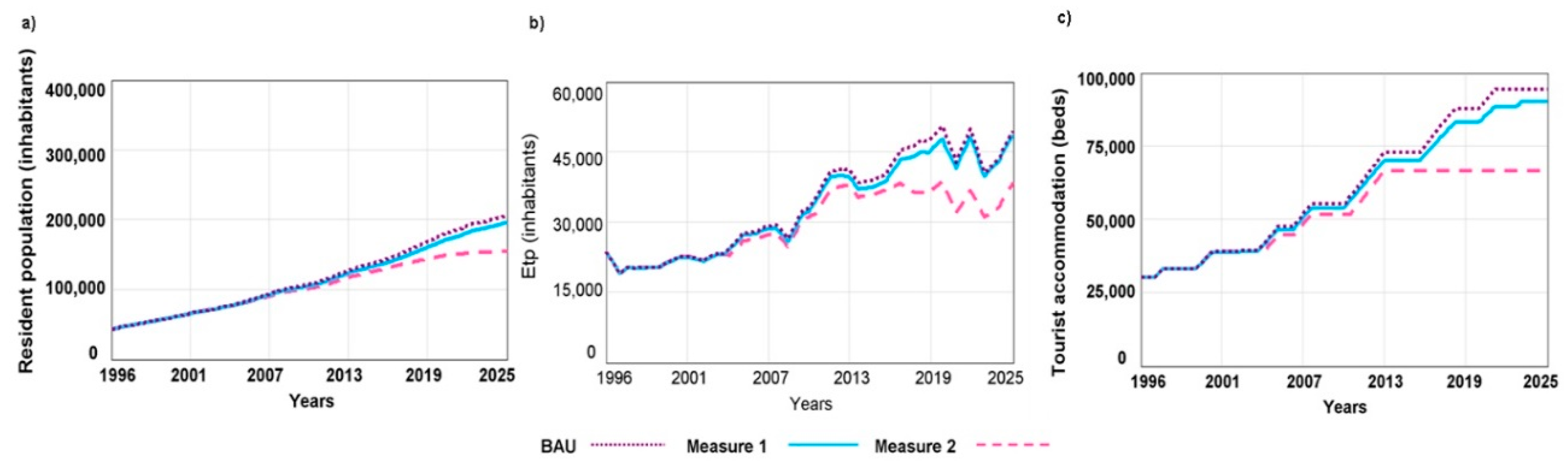
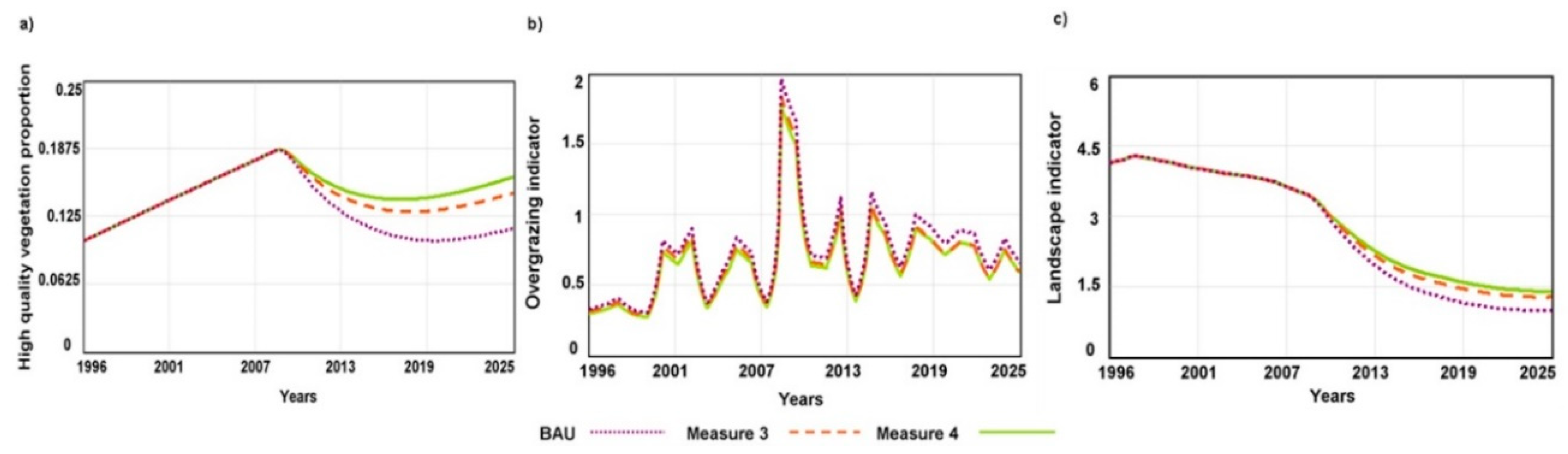
Regarding model application and, more specifically, the definition of policy measures, the sensitivity analysis (SA) has also allowed the identification of the leverage points of the model; that is, the parameters to whose changes the model is more responsive. The results point to the potential of using these leverage points to develop more effective measures, as compared with other measures with the same objective proposed by different agents. The greater effectiveness of leverage-based measures has been shown regarding the objectives of reducing grazing on the high quality natural vegetation and controlling the tourist accommodations growth. The SA has also allowed the explicit consideration and quantification of uncertainty in the assessment of policies. Conclusions regarding whether some objectives are achieved or not or, or whether certain sustainability thresholds might be exceeded or not, may change when uncertainty is taken into account. Monte Carlo simulations applied to the leverage-based policy measures showed that for several indicators their sustainability thresholds would not be exceeded when mean values are considered, but such thresholds might be surpassed when the uncertainty range with the 95% confidence bound is taken into account. Under the Business as Usual scenario, the number of indicators analyzed which would exceed their thresholds would increase from two to four out of seven. Under Policy I (limitation of new tourist accommodation) the number of indicators exceeding their thresholds would shift from one to three out of seven, whereas under Policy II (reduction of grazing to protect the soil and the high quality natural vegetation) the increase would be from three to four out of seven. Therefore, the potential risks related to the surpassing of sustainability thresholds may go unnoticed when the uncertainty is not considered.

To sum up, sensitivity analysis has been revealed as a powerful tool in all the stages of the model development and applications, and it is able to provide important insights to policy makers and end users regarding the sustainability of socio-ecological systems.

Supplementary Materials

The following are available online at https://www.mdpi.com/2071-1050/10/8/2928/s1, Table S1: Results of the One factor at a time (OAT) analysis; and the details of the mathematical formulation of the model.

Author Contributions

M.-A.E. had the original idea and contributed to the discussion of the study. P.E.-G. contributed to data collection. J.M.-F. contributed to the discussion. I.B.-G. contributed to calculation analysis, and both I.B.-G. and J.M.-F. wrote the paper. All authors have read and approved the final manuscript.

Funding

This research received no external funding.

Conflicts of Interest

The authors declare no conflict of interest.

Appendix A

Table A1. List of the parameters of the Fuerteventura sustainability dynamic model.

Parameters	Model Value (Units)	Definition	Range of Variation	References Regarding Range of Variation
ABROAD	0.74 (Dmnl)	Proportion of tourists arrived from abroad	0.66–0.83	[60]
AIR	0.1899 (Dmnl)	Accommodation increase ratio (Automatic Calibration, AC)	0.1424–0.2374	Standard range when no references (25%)
ARC	0.367 (Dmnl)	Adjustable runoff	0.2753–0.4588	Standard range when no references (25%)
AVERGOODS	1.2203 × 10⁹ (kg/year)	Average value of the Sea transportation of goods	0.763 × 10⁹–1.698 × 10⁹	[60]
AVERSTAY	9.06 (days)	Average length of the stay	7.53–11.11	[60]
B	33.2455 (Dmnl)	Intercept between births and GPDca	24.934–41.557	Standard range when no references (25%)
BIR BASE	−0.0188 (1/year)	Factor between births and GPDca	(−0.024)–(−0.014)	Standard range when no references (25%)
CFBUEU	3.37 (Dmnl)	Factor of urban built up which affects the houbara habitat	2.528–4.213	Standard range when no references (25%)
CO2FACTORgav	−300,000 (g CO₂/(year·ha))	CO₂ factor for gavias	(−300,000)–(−176,800)	[61,62]
CO2FACTORgc	−6.46 × 10⁶ (g CO₂/(year·ha))	CO₂ factor for golf courses	(−8.78 × 10⁶)–(−4.85 × 10⁶)	Standard range when no references (25%)
CO2FACTORirrig	−5 × 10⁶ (g CO₂/(year·ha))	CO₂ factor for irrigation area	(−6.25 × 10⁶)–(−3.75 × 10⁶)	Standard range when no references (25%)
CPRE	0.00082 (LU/(ha·mm))	Rainfall coefficient	0.00080–0.00084	Regression
desal CORRALEJO	1.46 × 10⁶ (m³/year)	Capacity of the desalination facilities in Corralejo	1.095 × 10⁶–1.825 × 10⁶	[63]
DIST1	316.14 (km/inhab)	Distance from Gran Canaria by passenger’s flights (round trip)	237.105–395.175	Standard range when no references (25%)
DIST2	3234.26 (km/inhab)	Distance from Madrid by passenger’s flights (round trip)	2425.695–4042.825	Standard range when no references (25%)
DIST3G	6973.66 (km/inhab)	Distance from Berlin by passenger’s flights (round trip)	5230.245–8717.075	Standard range when no references (25%)
DIST3UK	5604.92 (km/inhab)	Distance from London by passenger’s flights (round trip)	2101.845–3503.075	Standard range when no references (25%)
DIST4	2291.12 km/journey	Distance from Puerto de Cádiz to Puerto del Rosario (round trip)	1718.34–2863.9	Standard range when no references (25%)
DVEF	189.6 (g CO₂/kwh)	Diesel vehicles CO₂ emission factor	142.2–237	Standard range when no references (25%)
ECO2E	360 (g CO₂/kwh)	Electricity CO₂ emission factor	351–410	[64,65,66]
EECBR	829.495 (kwh/(inhab·year))	Population electric energy consumption base ratio, before considering the GPDca effect	622.1213–1036.8688	Standard range when no references (25%)
EICF	2 (MJ/km)	Energy intensity conversion factor	1.75–2.75	[67,68]
eLGCC	0.0215 Ev/LU	Effect of the livestock over the carrying capacity of the Egyptian vulture (AC)	0.016–0.027	Standard range when no references (25%)
EVAPORATION	67,000 (m³/year)	Annual evaporation rate from water reservoirs	30,150–67,000	[69]
EVTp	0.9 (Dmnl)	Evapotranspiration (after the improvement of model formulation by means of the SA, the model value is 0.315)	0.675–1.125	Standard range when no references (25%)
FCO₂E	69 (g CO₂/MJ)	Flights CO₂ emissions	69–71.6	[67]
FLOWSEAR	8.692 × 10⁻⁴ (1/year)	Volume flowing into sea ratio [69]	6.519 × 10⁻⁴–10.865 × 10⁻⁴	Insensitive parameters. Removed from the model structure after OAT.
FLOWSPRINGR	4.8751 × 10⁻⁶ (1/year)	Flow spring ratio [69]	3.656 × 10⁻⁶–6.094 × 10⁻⁶	Insensitive parameters. Removed from the model structure after OAT.
FODDER YIELD	37,705.5 (kg/(ha·year))	Annual fodder yield	17,178.2–37,705.5	[70,71]
FUEL CONSs	804.812 (kg fuel/km)	Fuel consumption of ships by each kilometer	740.43–869.2	[72]
GCR	0.0516 (1/year)	Gavias change ratio (AC)	0.0387–0.0644	Standard range when no references (25%)
GDPcaFACTOR	4240 (ships)	Effect of the GDPca on sea transportation of goods	2971–5509	Regression
GOLFCONR	10,950 (m³/(ha·year))	Golf courses water consumption	10,950–11,000	[73]
GOLFLOSR	0.2 (Dmnl)	Water loss in golf courses water supply	0.2–0.3	[74]
GVEF	95.312 (g CO₂/kwh)	Gasoline emission factor (vehicles)	71.48–119.14	Standard range when no references (25%)
HCRac	0.96 (Dmnl)	Houbara habitat change ratio due to active crops	0.73–1.21	Standard range when no references (25%)
HCRpermabandon	0.178 (Dmnl)	Houbara habitat change ratio due to permanent abandonment of gavias	0.134–0.223	Standard range when no references (25%)
HCRroads	15.509 (ha/km)	Houbara habitat change ratio due to roads	11.632–19.386	Standard range when no references (25%)
HCRtracks	8.42 (ha/km)	Houbara habitat change ratio due to tracks	6.315–10.525	Standard range when no references (25%)
HCRub	0.119 (Dmnl)	Houbara habitat change ratio per hectare of new urban built up	0.089–0.149	Standard range when no references (25%)
HOTEL ACCOMMODAT LAND DEM	0.0059 (ha/bed)	Demand of land by each nonhotel accommodation bed	0.0047–0.006	[75]
ICR	0.001103 (1/year)	Irrigation change rate (AC)	0.00083–0.00138	Standard range when no references (25%)
IR	0.062 (Dmnl)	Infiltration ratio from rainfall	0.052–0.062	[69,74,76]
IR gavias	0.2 (m/year)	Infiltration ratio in gavias	0.2–0.4	[69,74]
IRCONR	7000 (m³/(ha·year))	Irrigation consumption ratio	4631–7000	[69,74]
IRLOSR	0.43 (Dmnl)	Irrigation loss ratio	0.19–0.43	[74]
ISLAND	0.18 (Dmnl)	Proportion of tourist arrived from other island of the Archipelago	0.13–0.223	[60]
Kc	0.35 (Dmnl)	Cereal coefficient	0.3–0.4	Insensitive parameters, removed from the model structure after OAT
Kn	23.533 (Ev)	Egyptian vulture population carrying capacity natural, without considering the livestock effect	17.65–29.417	Standard range when no references (25%)
LOSS	0.31 (Dmnl)	Loss ratio for urban water supply	0.25–0.35	[69,74]
MAX ACCOMMODATION	133,000 (beds)	Maximum number of beds	133,000–283,935	[77] [78]
MF GDPca INMIG	1.24816 (Dmnl)	Effect of the GDPca on immigration (AC)	0.9361–1.5602	Standard range when no references (25%)
MFACTOR GDP	3.14604 (Dmnl)	Effect of the GDPreal on foreign tourists arrivals (AC)	2.3595–3.93255	Standard range when no references (25%)
MFACTOR IET	0.704086 (Dmnl)	Factor on the tourist choice index (AC)	0.5281–0.8801	Standard range when no references (25%)
MIR	0.6094 (1/year)	Maximum or intrinsic growth ratio for the Egyptian vulture (AC)	0.457–0.762	Standard range when no references (25%)
MOR	0.0036523 (1/year)	Mortality rate	0.0035–0.0037	[79]
NBEACH THRESHOLD	30 (m²/inhab)	Normalized beach factor threshold	10–30	[46,77]
NEEfactor	1.13987 × 10⁷(g CO₂/(year·ha))	Net ecosystem exchange factor	0.878 × 10⁷–1.402 × 10⁷	Regression
NGP	0.5 (Dmnl)	Net grazing proportion	0.29–0.5	[80]
NONHOT ACCOM LAND DEM	0.0042 (ha/bed)	Demand of land by each nonhotel accommodation bed	0.0035–0.007	[75]
NONHOT ACCOM RATIO	0.53 (1/year)	Nonhotel accommodations ratio regarding the total tourist accommodation.	0.25–0.68	[81]
NOTOURIST EMPLOY	0.249 (Dmnl)	Proportion of employment not linked to tourist	0.187–0.3111	Insensitive parameters. Removed from the model structure after OAT
PEGcpl	2.425 × 10⁻⁵(1/(km·year))	Probability of electrocution with corrective measures in power lines	1.819 × 10⁻⁵–3.031 × 10⁻⁵	Standard range when no references (25%)
PEGspl	9.7 × 10⁻⁵ (1/(km·year))	Probability of electrocution without corrective measures in power lines	7.275 × 10⁻⁵–12.125 × 10⁻⁵	Standard range when no references (25%)
PENINSULA	0.078 (Dmnl)	Proportion of tourist arrived from the Iberian Peninsula	0.021–0.136	[60]
PLRpc	0.00335 (km/inhab)	Power lines Ratio per capita	0.0024–0.0035	[82]
preFACTOR	−2.25604 × 10⁶ ((g CO₂)/(year·ha·mm)	Rainfall factor on the NEE	(−2.775 × 10⁶) –(−1.737 × 10⁶)	Regression
ptotFACTOR	0.000326 (ships/inhab)	Effect of the total population on the sea transportation of goods factor	0.000245–0.000408	Standard range when no references (25%)
ratioG	0.61 (Dmnl)	Proportion of German tourists from the foreign total tourists	0.52–0.63	[60]
ratioUK	0.38 (Dmnl)	Proportion of United Kingdom tourist from the total foreign tourists arrived to Fuerteventura	0.32–0.39	[60]
REUSR	0.35 (Dmnl)	Ratio of reusing urban reclaimed water	0–0.9	[74]
ROADSn	0.000358 (km/inhab/year)	New roads demand ratio	0.00027–0.00045	Standard range when no references (25%)
RPOPAQUIFR	0.01 (Dmnl)	Population Water demand from aquifer ratio	0.01–0.12	[69,74]
RPOPCONRbase	65.7 (m³/(year·inhab)	Residential population consumption ratio	55.72–65.7	[69,74]
RPSEWAGEPROP	0.6 (Dmnl)	Sewage proportion	0.45–0.75	Standard range when no references (25%)
RPTREATMENTP	0.91 (Dmnl)	Treatment water proportion from resident population.	0.73–0.9	[73,74]
RT	136.75 (years)	Average time of plant composition recovery (AC)	40–200	[83,84]
RUNOFFcte	0.026 (Dmnl)	Runoff constant	0.025–0.026	[85]
SCG	44 (ha/golf course)	Area occupied by golf course	40–45	[82]
SCO₂E	3200 (g CO₂/kg fuel)	Ships CO₂ Emission Factor	3170–3200	[86]
SEADES CONVR	0.45 (Dmnl)	Seawater desalination conversion ratio	0.45–0.55	[87,88,89]
SEADESCAP	2.757 × 10⁷ (m³/year)	Seawater desalination capacity	2.068 × 10⁷–3.446 × 10⁷	Insensitive parameters. Removed from the model structure after OAT
SEWAGE PROP TUR	0.57 (Dmnl)	Proportion of sewage water from tourist consumption	0.57–0.6	[90]
SFACTOR	691.1 (ships)	Ships factor. Intercept ships	476.9–905.3	Regression
shipCAPACITY	2.566 × 10⁹ (kg/ships)	Ship carrying capacity for goods	1.925 × 10⁹–3.208 × 10⁹	Standard range when no references (25%)
ST	79 (year)	Period of succession after the abandonment of agricultural areas	52–79	[91]
TCEO	0.254 (Dmnl)	Electric energy consumption ratio by other sectors	0.254–0.3	[92]
TCEOne	0.27 (Dmnl)	Non electric energy consumption ratio by other sectors	0.2025–0.3375	Standard range when no references (25%)
TCNE	333.302 (kwh/(inhab·year))	Non electric energy consumption ratio by population	249.977–416.628	Standard range when no references (25%)
TCONBOV	17.3 (m³/head of livestock)	Water consumption by each head of livestock (cows)	3.65–17.3	Insensitive parameters. Removed from the model structure after OAT.
TCONCAPROV	1.825 (m³/head of livestock)	Water consumption by each head of livestock (goats and sheep)	1.825–2	[69]
TCONPORC	2.87 (m³/head of livestock)	Water consumption by each head of livestock (pigs)	2.87–3.65	[69]
TCV	13,816.1 ((kwh/(car·year))	Annual energy consumption ratio by each car	13,816.1–17,124.519	[58]
TEMIG BASE	0.084 (1/year)	Base emigration ratio	0.071–0.092	[79]
TES	6.405 (year)	Time to detect the overgrazing effects (AC)	4.804–8.006	Standard range when no references (25%)
TGEREURBpc	589.28 (kg/(inhab·year))	Urban waste generation per capita	569.4–589.28	[77]
THRESHOLD OR	0.5305 (inhab/bed)	Profitability threshold for the occupancy rate.	0.5305–0.75	[46]
TINGBOV	16,607.5 (kg/(head·year))	Fodder consumption by each head of livestock (cows)	15,695–17,520	Insensitive parameters. Removed from the model structure after OAT.
TINGCAPROV	657 (kg/(head·year))	Fodder consumption by each head of livestock (goats and sheep)	657–730	[93]
TINGPORC	1124.2 (kg/(head·year))	Fodder consumption by each head of livestock (pigs)	886.95–1343.2	Insensitive parameters. Removed from the model structure after OAT.
TINMIGDPca	2 (year)	Time of the effect of the GDPca on the immigration (AC)	1.5–2.5	Standard range when no references (25%)
TKWM3	4.5 (kwh/m³)	Energy consumption for desalination	3.123–5.877	[87,88]
TMOTN	0.421658 (car/inhab)	Motorization index base (AC)	0.316–0.527	Standard range when no references (25%)
TPP	1 (Dmnl)	Non electric energy loss ratio (from primary energy to final energy)	0.75–1.25	Standard range when no references (25%)
TRACKSn	0.001719 (km/inhab/year)	New tracks demand ratio	0.0013–0.0022	[82]
TRECRES	0.07 (Dmnl)	Recycled waste ratio from the mixture of waste.	0.048–0.111	[82]
TRECSELEC	49.57 (kg/(inhab·year))	Selective urban solid wastes collection ratio.	31.65–54.4	[82]
TSUCVOpc	0.074 (ha/(inhab·year))	Built Urban and other uses per house ratio (AC)	0.064–0.074	Standard range when no references (25%)
TURCONR	126.02 (m³ /(inhab·year))	Tourist water consumption ratio	101–126.02	[74,77]
WCO₂E	2200 (g CO₂/kg)	Waste CO₂ Emission factor	1650–2750	Standard range when no references (25%)

Table A2. Detailed results of the goodness of fit tests for the 20 variables with available observed data series, before and after removing the insensitive parameters.

Variables	n	Results for Calibration Period before Removing Insensitive Parameters		Results after Removing Insensitive Parameters
Variables	n	MAPE (%)	RMSE (%)	MAPE (%)	RMSE (%)
Resident population	16	4.30	5.45	4.30	5.45
Births	12	6.22	5.62	6.22	5.62
Immigration	16	26.18	23.38	26.18	23.38
Emigration	15	32.70	31.65	32.70	31.65
Tourist equivalent population	16	9.52	12.03	9.52	12.03
Tourist accommodation capacity	16	7.29	9.4	7.29	9.4
Occupancy rate	16	8.71	10.84	8.71	10.84
Tourist employment	13	5.39	6.63	5.39	6.63
Houbara habitat	3	0.98	1.53	0.98	1.53
Egyptian vulture population	13	4.54	5.08	4.54	5.08
Urban built-up	16	2.34	2.84	2.34	2.84
Tracks	3	1.06	1.73	1.06	1.73
Roads	3	0.71	1.05	0.71	1.05
Active crops area	15	10.14	11.40	10.14	11.40
Irrigated crops area	15	11.76	13.70	11.76	13.70
Active gavias area	15	10.49	11.55	10.49	11.55
Natural vegetation area	3	0.28	0.45	0.28	0.45
Golf courses area	15	10.01	24.45	10.01	24.45
Vehicles fleet	12	4.57	4.15	4.57	4.15
Electric energy consumption	14	4.98	7.14	4.98	7.14

n: Number of observed data.

Table A3. Model formulation of the 7 selected sustainability indicators.

Indicators	Equations	Variables Involved
Ratio of tourists to residents (tures)	$t u r e s = \frac{e t p}{r e s}$	etp: equivalent tourist population. res: resident population.
Ratio between tourist accommodations and resident population (ear)	$e a r = \frac{t a c}{r e s}$	tac: tourist accommodation capacity. res: resident population.
Artificial land percentage (alp)	$a l p = \frac{r e a + h o t + n h o + g o f + r o d + t r a + i r r}{F v a} \times 100$	rea: area occupied by residential uses. hot: area occupied by hotels and their facilities. nho: area occupied by non-hotels and their facilities. gof: area occupied by golf courses. rod: area occupied by roads. tra: area occupied by tracks or unpaved roads. irr: area occupied by irrigation lands. Fva: Fuerteventura island area.
High quality vegetation proportion (hqp)	$h q p = \frac{h q v}{t o t v}$	hqv: high quality natural vegetation area. totv: total natural vegetation.
Overgrazing indicator (oi)	$o i = (\frac{l s \cdot n g p}{r f \cdot s r c})$	ls: livestock of the island. ngp: net grazing proportion. rf: rainfall. src: sustainable stocking rate capacity.
Houbara habitat proportion (hhp)	$h h p = \frac{(c h_{a g} \cdot H P_{a g}) + (p a r \cdot H P_{p a}) - (b u \cdot H P_{b u}) - (n r \cdot H P_{n r}) - (n t \cdot H P_{n t})}{h h_{r e f}}$	chag: annual changes in abandoned gavias area (from and to active gavias). HPag is the proportion of abandoned gavias which is part of the habitat. par: the abandoned gavias to natural vegetation succession rate. HPpa: the proportion of natural vegetation which is part of the habitat. bu: the annual change of urban areas. HPbu: the proportion of these urban areas which negatively affect the habitat. nr and nt: the new paved roads and unpaved tracks which annually appear on the island, respectively. HPnr and HPnt: the proportion of the new roads and tracks which negatively affect the habitat, respectively. hhref: reference value.
Egyptian vulture population proportion (Evp)	$E v p = \frac{(e v \cdot m i r \cdot \frac{k + k_{l s} - e v}{k + k_{l s}}) - ((e p \cdot p l i \cdot e v + f_{s t k}) + p o s)}{e v_{r e f}}$	ev: population of the Egyptian vulture. mir: is the maximum or intrinsic growth ratio for the Egyptian vultures. k: Egyptian vulture carrying capacity without considering the livestock effect. kls: the additional carrying capacity generated by the existence of livestock. ep: the probability of electrocution. pli: the length of power lines on the island. fstk: the stochastic factor included in the electrocution probability. pos: refers to poisonings. evref: reference data of the population of the Egyptian vulture.

References

Hodbod, J.; Adger, W.N. Integrating social-ecological dynamics and resilience into energy systems research. Energy Res. Soc. Sci. 2014, 1, 226–231. [Google Scholar] [CrossRef]
Kelly, R.A.; Jakeman, A.J.; Barreteau, O.; Borsuke, M.E.; ElSawah, S.; Hamilton, S.H.; Henriksen, H.S.; Kuikka, S.; Maier, H.R.; Rizzoli, A.E.; et al. Selecting among five common modelling approaches for integrated environmental assessment and management. Environ. Model. Softw. 2013, 47, 159–181. [Google Scholar] [CrossRef]
Martínez-Moyano, I.J.; Richardson, G.P. Best practices in system dynamics modeling. Syst. Dyn. Rev. 2013, 29, 102–123. [Google Scholar] [CrossRef]
Bodde, M.; van der Wel, K.; Driessen, P.; Wardekker, A.; Runhaar, H. Strategies for Dealing with Uncertainties in Strategic Environmental Assessment: An Analytical Framework Illustrated with Case Studies from The Netherlands. Sustainability 2018, 10, 2463. [Google Scholar] [CrossRef]
Hou, Y.; Burkhard, B.; Müller, F. Uncertainties in landscape analysis and ecosystem service assessment. J. Environ. Manag. 2013, 127, S117–S131. [Google Scholar] [CrossRef] [PubMed]
Ascough, J.C.; Maier, H.R.; Ravalico, J.K.; Strudley, M.W. Future research challenges for incorporation of uncertainty in environmental and ecological decision-making. Ecol. Model. 2008, 219, 383–399. [Google Scholar] [CrossRef]
Warmink, J.J.; Janssen, J.A.E.B.; Booij, M.J.; Krol, M.S. Identification and classification of uncertainties in the application of environmental models. Environ. Model. Softw. 2010, 25, 1518–1527. [Google Scholar] [CrossRef]
Pianosi, F.; Beven, K.; Freer, J.; Hall, J.W.; Rougier, J.; Stephenson, D.B.; Wagener, T. Sensitivity analysis of environmental models: A systematic review with practical workflow. Environ. Model. Softw. 2016, 79, 214–232. [Google Scholar] [CrossRef] [Green Version]
Holzkämper, A.; Klein, T.; Seppelt, R.; Fuhrer, J. Assessing the propagation of uncertainties in multi-objective optimization for agro-ecosystem adaptation to climate change. Environ. Model. Softw. 2015, 66, 27–35. [Google Scholar] [CrossRef]
Gong, W.; Duan, Q.Y.; Li, J.D.; Wang, C.; Di, Z.H.; Ye, A.Z.; Miao, C.Y.; Dai, Y.J. An intercomparison of sampling methods for uncertainty quantification of environmental dynamic models. J. Environ. Inf. 2016, 28, 11–24. [Google Scholar] [CrossRef]
Jakeman, A.J.; Letcher, R.A. Integrated assessment and modelling: Features, principles and examples for catchment management. Environ. Model. Softw. 2003, 18, 491–501. [Google Scholar] [CrossRef]
Brown, S. Foreign aid and democracy promotion: Lessons from Africa. Eur. J. Dev. Res. 2005, 17, 179–198. [Google Scholar] [CrossRef]
Schouten, M.; Verwaart, T.; Heijman, W. Comparing two sensitivity analysis approaches for two scenarios with a spatially explicit rural agent-based model. Environ. Model. Softw. 2014, 54, 196–210. [Google Scholar] [CrossRef]
Banos-González, I.; Martínez-Fernández, J.; Esteve, M.A. Dynamic integration of sustainability indicators in insular socio-ecological systems. Ecol. Model. 2015, 306, 130–144. [Google Scholar] [CrossRef]
Banos-González, I.; Martínez-Fernández, J.; Esteve, M.A. Using dynamic sustainability indicators to assess environmental policy measures in Biosphere Reserves. Ecol. Indic. 2016, 67, 565–576. [Google Scholar] [CrossRef]
Santana-Jiménez, Y.; Hernández, J.M. Estimating the effect of overcrowding on tourist attraction: The case of Canary Islands. Tourism Manag. 2011, 32, 415–425. [Google Scholar] [CrossRef]
Action Plan of the Fuerteventura Biosphere Reserve. Available online: http://gestion.cabildofuer.es/fuerteventurabiosfera/ (accessed on 4 November 2013).
Rodríguez-Rodríguez, A.; Mora, J.L.; Arbelo, C.; Bordon, J. Plant succession and soil degradation in desertified areas (Fuerteventura, Canary Islands, Spain). Catena 2005, 59, 117–131. [Google Scholar] [CrossRef]
Dorta-Santos, M.; Tejedor, M.; Jiménez, C.; Hernández-Moreno, J.M.; Palacios, M.P.; Díaz, F.J. Recycled urban wastewater for irrigation of Jatropha curcas L. in abandoned agricultural arid land. Sustainability 2014, 6, 6902–6924. [Google Scholar] [CrossRef]
Donázar, J.A.; Palacios, C.J.; Gangoso, L.; Ceballos, O.; González, M.J.; Hiraldo, F. Conservation status and limiting factors in the endangered population of Egyptian vulture (Neophron percnopterus) in the Canary Islands. Biol. Conserv. 2002, 107, 89–97. [Google Scholar] [CrossRef]
Carrascal, L.M.; Palomino, D.; Seoane, J.; Alonso, C.L. Habitat use and population density of the houbara bustard Chlamydotis undulata in Fuerteventura (Canary Islands). Afr. J. Ecol. 2008, 46, 291–302. [Google Scholar] [CrossRef] [Green Version]
Forrester, J.W. Industrial Dynamics; The MIT Press: Cambridge, MA, USA, 1961. [Google Scholar]
Wang, X.; Yao, M.; Li, J.; Zhang, K.; Zhu, H.; Zheng, M. China’s rare earths production forecasting and sustainable development policy implications. Sustainability 2017, 9, 1003. [Google Scholar] [CrossRef]
Banos-González, I.; Terrer, C.; Martínez-Fernández, J.; Esteve-Selma, M.A.; Carrascal, L.M. Dynamic modelling of the potential habitat loss of endangered species: The case of the Canarian houbara bustard (Chlamydotis undulata fuertaventurae). Eur. J. Wildl. Res. 2016, 62, 263–275. [Google Scholar] [CrossRef]
Oliva, R. Model calibration as a testing strategy for system dynamics models. Eur. J. Oper. Res. 2003, 151, 552–568. [Google Scholar] [CrossRef]
Makler-Pick, V.; Gal, G.; Gorfine, M.; Hipsey, M.R.; Carmel, Y. Sensitivity analysis for complex ecological models–a new approach. Environ. Model. Softw. 2011, 26, 124–134. [Google Scholar] [CrossRef]
Barlas, Y. Formal aspects of model validity and validation in system dynamics. Sys. Dyn. Rev. J. Syst. Dyn. Soc. 1996, 12, 183–210. [Google Scholar] [CrossRef]
Uusitalo, L.; Lehikoinen, A.; Helle, I.; Myrberg, K. An overview of methods to evaluate uncertainty of deterministic models in decision support. Environ. Model. Softw. 2015, 63, 24–31. [Google Scholar] [CrossRef]
Holmes, G.; Johnstone, R.W. Modelling coral reef ecosystems with limited observational data. Ecol. Model. 2010, 221, 1173–1183. [Google Scholar] [CrossRef]
Sun, X.Y.; Newham, L.T.H.; Croke, B.F.W.; Norton, J.P. Three complementary methods for sensitivity analysis of a water quality model. Environ. Model. Softw. 2012, 37, 19–29. [Google Scholar] [CrossRef]
Moreau, P.; Viaud, V.; Parnaudeau, V.; Salmon-Monviola, J.; Durand, P. An approach for global sensitivity analysis of a complex environmental model to spatial inputs and parameters: A case study of an agro-hydrological model. Environ. Model. Softw. 2013, 47, 74–87. [Google Scholar] [CrossRef]
Gao, L.; Bryan, B.A.; Nolan, M.; Connor, J.D.; Song, X.; Zhao, G. Robust global sensitivity analysis under deep uncertainty via scenario analysis. Environ. Model. Softw. 2016, 76, 154–166. [Google Scholar] [CrossRef]
Ventana System (Vensim ®, Ventana System, Inc.). Available online: http://www.vensim.com (accessed on 10 August 2018).
Ford, A. Estimating the impact of efficiency standards on the uncertainty of the Northwest electric system. Oper. Res. 1990, 38, 580–597. [Google Scholar] [CrossRef]
Ford, A.; Flynn, H. Statistical screening of system dynamic models. Syst. Dyn. Rev. J. Syst. Dyn. Soc. 2005, 21, 273–303. [Google Scholar] [CrossRef]
Jørgensen, S.E.; Fath, B. Fundamentals of Ecological Modelling, 4th ed.; Elsevier: Amsterdam, The Netherlands, 2011; p. 400. [Google Scholar]
Graham, A.K.; Moore, J.; Choi, C.Y. How robust are conclusions from a complex calibrated model, really? A project management model benchmark using fit-constrained Monte Carlo analysis. In Proceedings of the 20th System Dynamics Conference of the System Dynamics Society, Palermo, Italy, 28 July–1 August 2002. [Google Scholar]
Hekimoğlu, M.; Barlas, Y. Sensitivity analysis of system dynamics models by behavior pattern measures. In Proceedings of the 28th International Conference of the System Dynamics Society, System Dynamics Society, Albany, NY, USA, 25–29 July 2010. [Google Scholar]
Lesnoff, M.; Corniaux, C.; Hiernaux, P. Sensitivity analysis of the recovery dynamics of a cattle population following drought in the Sahel region. Ecol. Model. 2012, 232, 28–39. [Google Scholar] [CrossRef]
Grant, W.E.; Swannack, T.M. Ecological Modelling. A Common-Sense Approach to Theory and Practice; Blackwell Publishing: Oxford, UK, 2008. [Google Scholar]
Meadows, D. Leverage Points Places to Intervene in a System; Sustainability Institute: Hartland, VT, USA, 1999. [Google Scholar]
Voinov, A.; Bousquet, F. Modelling with stakeholders. Environ. Model. Softw. 2010, 25, 1268–1281. [Google Scholar] [CrossRef]
Moeller, C.; Sauerborn, J.; de Voil, P.; Manschadi, A.M.; Pala, M.; Meinke, H. Assessing the sustainability of wheat-based cropping systems using simulation modelling: Sustainability= 42? Sustain. Sci. 2013, 1–16. [Google Scholar] [CrossRef]
UNESCO (Man and Biosphere Program). Available online: http://www.unesco.org/new/en/natural-sciences/environment/ecological-sciences/biosphere-reserves/europe-north-america/spain/fuerteventura/ (accessed on 27 December 2009).
Stankey, G.H.; Cole, D.N.; Lucas, R.C.; Petersen, M.E.; Frissell, S.S. The Limits of Acceptable Change (LAC) System for Wilderness Planning; USDA Forest Service, Intermountain Forest and Range Experiment Station: Ogden, UT, USA, 1985. [Google Scholar]
Government of Canary Islands. Metodología para la Aplicación Práctica de la Apreciación y Evaluación de los Factores Determinantes de la Capacidad de Carga. Especialmente en Zonas Turísticas. Consejería de Medio Ambiente y Ordenación Territorial; Government of the Canary Islands. Available online: http://www.fecam.es/documentos/areas/turismo_transportes/CCTGuia.pdf (accessed on 17 December 2014).
Graymore, M.L.; Sipe, N.G.; Rickson, R.E. Sustaining human carrying capacity: A tool for regional sustainability assessment. Ecol. Econ. 2010, 69, 459–468. [Google Scholar] [CrossRef]
Government of Canary Islands. Law 19/2003, on 14th. April 2003, on Arrangement of Territory and Tourism of the Canary Islands; Government of the Canary Islands: The Canary Islands, Spain, 2003.
Fuerteventura Cabildo. Available online: http://www.cabildofuer.es/documentos/Medio_ambiente/subvenciones/gavias/plan_estrategico_subvencion_gavias.pdf (accessed on 6 September 2014).
Mata, J.; Flores, M.P.; Camacho, A.; Delgado-Bermejo, J.V.; Bermejo, L.A. Uso Ganadero del Parque Rural de Anaga. Resultados Preliminares; Arch. Zootec.; Universidad de Córdoba, Servicio de Publicaciones: Madrid, Spain, 2000; Volume 49, pp. 269–274. [Google Scholar]
Muleta, M.K.; Nicklow, J.W. Sensitivity and uncertainty analysis coupled with automatic calibration for a distributed watershed model. J. Hydrol. 2005, 306, 127–145. [Google Scholar] [CrossRef]
Perz, S.G.; Muñoz-Carpena, R.; Kiker, G.; Holt, R.D. Evaluating ecological resilience with global sensitivity and uncertainty analysis. Ecol. Model. 2013, 263, 174–186. [Google Scholar] [CrossRef]
Xing, Y.; Dangerfield, B. Modelling the sustainability of mass tourism in island tourist economies. J. Oper. Res. Soc. 2011, 62, 1742–1752. [Google Scholar] [CrossRef]
Von Bergner, N.M.; Lohmann, M. Future Challenges for Global Tourism: A Delphi Survey. J. Travel Res. 2014, 5, 420–432. [Google Scholar] [CrossRef]
Sterk, B.; Carberry, P.; Leeuwis, C.; van Ittersum, M.K.; Howden, M.; Meinke, H.; van Keulen, H.; Rossing, W.A.H. The interface between land use systems research and policy: Multiple arrangements and leverages. Land Use Policy 2009, 26, 434–442. [Google Scholar] [CrossRef]
Baroni, G.; Tarantola, S. A General Probabilistic Framework for uncertainty and global sensitivity analysis of deterministic models: A hydrological case study. Environ. Model. Softw. 2014, 51, 26–34. [Google Scholar] [CrossRef]
Oreja-Rodríguez, J.R.; Parra-López, E.; Yanes-Estévez, V. The sustainability of island destinations: Tourism area life cycle and teleological perspectives. The case of Tenerife. Tourism Manag. 2008, 29, 53–65. [Google Scholar] [CrossRef]
Martín-Cejas, R.; Ramírez Sánchez, P. Ecological footprint analysis of road transport related to tourism activity: The case for Lanzarote Island. Tourism Manag. 2010, 31, 98–103. [Google Scholar] [CrossRef]
Mori, K.; Christodoulou, A. Review of sustainability indices and indicators: Towards a new City Sustainability Index (CSI). Environ. Impact Assess. Rev. 2012, 32, 94–106. [Google Scholar] [CrossRef]
Instituto Canario de Estadística (ISTAC). Tourism Demand: Tourists and Passengers (1993–2015); ISTAC: Las Palmas, Spain. Available online: http://www.gobiernodecanarias.org/istac/temas_estadisticos/sectorservicios/hosteleriayturismo/demand/C00017A.html (accessed on 20 January 2016).
Díaz, F.; Jiménez, C.C.; Tejedor, M. Nutrient balance in water harvesting soils. Soc. Nat. 2005, 1, 522–537. [Google Scholar]
Padilla, F.M.; Vidal-Legaz, B.; Sánchez, J.; Pugnaire, F.I. Land-use changes and carbon sequestration through the twentieth century in a Mediterranean mountain ecosystem: Implications for land management. J. Environ. Manag. 2010, 91, 2688–2695. [Google Scholar] [CrossRef] [PubMed]
Renforus Renewable Energy Futures for Unesco Sites. Available online: http://195.76.147.227/renforus/site/pdf/GOOD%20PRACTICES/FUERTEVENTURA-REF.pdf (accessed on 6 September 2014).
Castellani, V.; Sala, S. Sustainability indicators integrating consumption patterns in strategic environmental assessment for urban planning. Sustainability 2013, 5, 3426–3446. [Google Scholar] [CrossRef]
Alacid, M.; Castellar, M.R.; Obón de Castro, J.M. La electricidad, ¿una energía limpia? Cálculos estequiométricos y termoquímicos a partir de la información de la factura de la luz. In Proceedings of the II Jornadas Sobre la Enseñanza de Las Ciencias y Las Ingenierías, Murcia, Spain, 1 November 2010. [Google Scholar]
Trappey, A.J.; Trappey, C.V.; Lin, G.Y.; Chang, Y.S. The analysis of renewable energy policies for the Taiwan Penghu island administrative region. Renew. Sustain. Energy Rev. 2012, 16, 958–965. [Google Scholar] [CrossRef]
Becken, S. Analysing international tourist flows to estimate energy use associated with air travel. J. Sustain. Tourism 2002, 10, 114–131. [Google Scholar] [CrossRef]
Hunter, C.; Shaw, J. The ecological footprint as a key indicator of sustainable tourism. Tourism Manag. 2007, 28, 46–57. [Google Scholar] [CrossRef]
Fuerteventura Island Water Plan (HPF). BOC nº 105, Viernes 6 de Agosto de 1999: 1408. DECRETO 81/1999 de 6 de Mayo, por el que se Aprueba el Plan Hidrológico Insular de Fuerteventura: Consejería de Obras Públicas, Vivienda y Aguas; Gobierno de Canarias: The Canary Islands, Spain, 1999. [Google Scholar]
Palacios, M.P.; Mendoza-Grimon, V.; Fernández, F.; Fernández-Vera, J.R.; Hernández-Moreno, J.M. Sustainable reclaimed water management by subsurface drip irrigation system: A study case for forage production. Water Pract. Technol. 2008, 3. [Google Scholar] [CrossRef]
Instituto Canario de Estadística (ISTAC). Agriculture. ISTAC: Las Palmas, Spain. Available online: http://www.gobiernodecanarias.org/istac/temas_estadisticos/sectorprimario/agricultura/agricultura (accessed on 20 January 2016).
Grupo de Investigación del Transporte Marítimo de la Fundación Universidad de Oviedo. Energy Consumption and Emission Associated with Transportation by Ship. Available online: http://www.investigacion-ffe.es/documentos/enertrans/EnerTrans_Consumos_barco.pdf (accessed on 14 September 2014).
Fuerteventura Cabildo. Estudio Capacidad de Carga de la Revisión del Plan Insular de Ordenación de Fuerteventura; Cabildo de Fuerteventura: Gran Canaria, Spain, 2013; p. 87. [Google Scholar]
Fuerteventura island Water Plan (HPF). Informative Report. Consejo Insular de Aguas de Fuerteventura. Available online: http://www.aguasfuerteventura.com/documentos/plan_hidrologico/Memoria_Informativa.pdf (accessed on 6 January 2016).
Government of Canary Islands. Estudios previos y selección de área turísticas degradadas de actuación, de carácter general y urbanístico; Área del casco tradicional de Corralejo en Fuerteventura: Gran Canaria, Spain, 2004.
Cabrera, M.C.; Custodio, E. The canary island. In Water, Agriculture and the Environment in Spain: Can We Square the Circle? De Stefano, L., Llamas, M.R., Eds.; CRC Press: Leiden, The Netherlands, 2012; pp. 281–291. [Google Scholar]
PTEOIEFTV [Special Territorial Plan for Energy Facilities Management of Fuerteventura]. Available online: http://www.gobiernodecanarias.org/energia/doc/pteoie/FUERTEVENTURA/03_MEN_ORD/1516_Mem_ord_PTEOIE_FTV_2008_04_09.pdf (accessed on 17 January 2014).
Gallardo, A.; Cáceres, Y. Reserva de Biosfera de Fuerteventura: Una Alterantiva al Modelo Turístico Tradicional. In Proceedings of the Conama 10: Congreso Nacional del Medio Ambiente (Technical Report), Madrid, 22–26 November 2010; Available online: http://www.conama10.conama.org/conama10/download/files/CT%202010/1000000175.pdf (accessed on 14 September 2014).
Instituto Canario de Estadística (ISTAC). Demographics Figures (1991–2010); ISTAC: Las Palmas, Spain. Available online: http://www.gobiernodecanarias.org/istac/temas_estadisticos/demografia/poblacion/cifraspadronales/ (accessed on 17 January 2014).
Mata, J.; Bermejo, L.A.; Delgado, J.V.; Camacho, A.; Flores, M.P. Estudio del uso ganadero en espacios protegidos de canarias. Metodología. Arch. Zootec. 2000, 49, 275–284. [Google Scholar]
Government of Canary Islands. Viceconsejería de Turismo. Observatorio Turístico: Estadísticas y Estudios. Alojativos: Establecimientos y Plazas Autorizadas. Available online: http://www.gobiernodecanarias.org/presidencia/turismo/estadisticas_y_estudios/Pasajeros_procedentes_del_extranjero_segxn_Pais_de_origen_/index-bis.html (accessed on 16 September 2015).
GRAFCAN (Homepage on the Internet). Available online: http://www.idecan.grafcan.es (accessed on 10 November 2015).
Otto, R.; Krüsi, B.O.; Burga, C.A.; Fernández-Palacios, J.M. Old-field succession along a precipitation gradient in the semi-arid coastal region of Tenerife. J. Arid Environ. 2006, 65, 156–178. [Google Scholar] [CrossRef]
Tzanopoulos, J.; Mitchley, J.; Pantis, J.D. Vegetation dynamics in abandoned crop fields on a Mediterranean island: Development of succession model and estimation of disturbance thresholds. Agric. Ecosyst. Environ. 2007, 120, 370–376. [Google Scholar] [CrossRef]
Instituto Tecnológico Geominero de España (ITGE). Estudio Hidrogeológico de la Isla de Fuerteventura. Memoria. Estudio Correspondiente al “Proyecto de Actualización Infraestructura Hidrogeológica, Vigilancia y Catálogo de Acuíferos. Años 1988/89/90”; Ministerio de Industria, Comercio y Turismo: Madrid, Spain, 1990; p. 194.
Deniz, C.; Kilic, A. Estimation and assessment of shipping emissions in the region of Ambarlı Port, Turkey. Environ. Prog. Sustain. Energy 2010, 29, 107–115. [Google Scholar] [CrossRef]
Von Medeazza, G.M.; Moreau, V. Modelling of water–energy systems. The case of desalination. Energy 2007, 32, 1024–1031. [Google Scholar] [CrossRef]
Meneses, M.; Pasqualino, J.C.; Céspedes-Sánchez, R.; Castells, F. Alternatives for reducing the environmental impact of the main residue from a desalination plant. J. Ind. Ecol. 2010, 14, 512–527. [Google Scholar] [CrossRef]
Pérez-González, A.; Urtiaga, A.M.; Ibáñez, R.; Ortiz, I. State of the art and review on the treatment technologies of water reverse osmosis concentrates. Water Res. 2012, 46, 267–283. [Google Scholar] [CrossRef] [PubMed]
Consejo Insular de Aguas de Gran Canaria (CIAGC). Estudio Hidrogeológico Para la Definición de Áreas Sobreexplotadas o en Riesgo de Sobreexplotación en la Zona Baja del Este de Gran Canaria. Convenio Específico 1998–2003. Capitulo V. Recursos Hídricos no Convencionales. Consejo Insular de Aguas de Gran Canaria. Available online: http://www.aguasgrancanaria.com/ciagcweb/articulos.nsf/ed7d80e62e5c0d4680257398002fd43b/a784546aa23093be8025774400491d7c/$FILE/CAPITULO%20V.%20Recursos%20h%C3%ADdricos%20no%20convencionales.pdf (accessed on 23 September 2011).
Abella, R.S. Disturbance and Plant Succession in the Mojave and Sonoran Deserts of the American Southwest. Int. J. Environ. Res. Public Health 2010, 7, 1248–1284. [Google Scholar] [CrossRef] [PubMed] [Green Version]
Government of Canary Islands. Sectorización del Consumo de Energía Final en Canarias en el año 2006. Available online: http://www.gobcan.es/energia/doc/eficienciaenergetica/pure/sectorizacion.pdf (accessed on 20 September 2015).
Monzón-Gil, E. Productividad de Cabras de Raza Majorera en Régimen Intensivo con Suministro de dos Tipos de Raciones, Tradicionales y Mezclada. Ph.D. Thesis, Universidad de Las Palmas de Gran Canaria, Las Palmas, Spain, 2007. [Google Scholar]

Figure 1. Monte Carlo SA results for changes in the values of sensitive parameters (local sensitivity over 50%), for the following target model variables: (a) Built-up urban, (b) High quality vegetation proportion, (c) Gavias proportion, (d) Overgrazing indicator, (e) Fodder importation needs, (f) Resident population, (g) Equivalent tourist population, (h) Houbara habitat proportion, (i) Egyptian vultures proportion, (j) Electric energy consumption, (k) Share of renewable energy, (l) Per capita CO₂ emissions, (m) Groundwater recharge, (n) Groundwater pumping, (o) Desalinated water, (p) Brine production, (q) Treated sewage proportion, and (r) Recycled waste.

Figure 2. Simulation results under different measures for the following indicators: (a) resident population; (b) equivalent tourist population; and (c) tourist accommodation.

Figure 3. Simulation results under different measures for the following indicators: (a) high quality vegetation proportion; (b) overgrazing indicator and (c) landscape indicator. All of them are dimensionless.

Table 1. Selected indicators included in the Fuerteventura sustainability dynamic model and their thresholds.

Indicators	Units	Direction of Change	Threshold	Meaning of the Threshold	Sources of the Thresholds
Ratio of tourists to residents (tures)	Dimensionless	Less is better	<0.3152	The ratio of tourists to local inhabitants should be lower than the threshold.	[46]
Ratio of tourists accommodation to resident population (ear)	Touristic beds/inhabitant	Less is better	<0.97	Ratio of tourist accommodations to resident population.	[46]
Artificial land percentage (alp)	%	Less is better	<20	Percentage of modified land (agriculture, urban, infrastructures).	[47]
High quality vegetation proportion (hqp)	Dimensionless	More is better	LCA > 0.1394	0.139 is the Limit of Acceptable Change (75% of the 2009 value).	Model value in 2009.
Overgrazing indicator (oi)	Dimensionless	Less is better	<1	Values above 1 mean overgrazing.	[14]
Houbara habitat proportion (hhp)	Dimensionless	More is better	LCA > 0.75	0.75 is the Limit of Acceptable Change (75% of the 2009 value).	Model value in 2009.
Egyptian vulture population proportion (Evp)	Dimensionless	More is better	LCA > 0.75	0.75 is the Limit of Acceptable Change (75% of the 2009 value).	Model value in 2009.

Table 2. Results of the Monte Carlo sensitivity analysis. For each target variable, the most responsive parameters (Sensitivity index, S_i,j ≥ 50%) were used. See Table A1 for the meanings of the parameter acronyms.

Target Model Variable	Responsive Parameters	Sensitivity Results 95% Confidence Interval (in 2025)
Built-up urban (bu)	AIR, B, BIR BASE, MF GDPca INMIG, MFACTOR IET, THRESHOLD OR, TSUCVpc	10,335 ± 8042 (Hectares)
High quality vegetation prop (hqp)	CPRE, BIR BASE, MFACTOR IET, NGP, RT	0.141 ± 0.12 (Dimensionless)
Gavias proportion (gap)	GCR, REUSR	0.058 ± 0.0015 (Dimensionless)
Overgrazing indicator (oi)	CPRE, NGP	0.518 ± 0.125 (Dimensionless)
Fodder importation needs (fin)	NGP, TINGCAPROV, THRESHOLD OR	0.575 ± 0.088 (Dimensionless)
Resident population (respop)	AIR, B, BIR BASE, MF GDPca INMIG, MFACTOR IET, THRESHOLD OR	140,862 ± 118,391 (Inhabitants)
Equivalent tourist population (etp)	B, BIR BASE, MFACTOR IET, THRESHOLD OR	37,042 ± 17,705 (Inhabitants)
Houbara habitat proportion (hhp)	BIR BASE, MFACTOR IET, THRESHOLD OR	0.738 ± 0.213 (Dimensionless)
Egyptian vulture proportion (Evp)	NGP, eLGCC	1.113 ± 0.263 (Dimensionless)
Electric energy consumption (enc)	B, BIR BASE, MFACTOR IETTHRESHOLD OR, EECBR, TCEO	1030 ± 0.721 (Mwh/year)
Share of renewable energy (SER)	B, BIR BASE, MFACTOR IET, TCV, THRESHOLD OR, TMONT, TPP	0.011 ± 0.006 (%)
Per capita CO₂ emissions (CO₂ pc)	NEEfactor, preFACTOR, MFACTOR IET, THRESHOLD OR, AVERGOODS, FUEL CONSs	32.2 ± 37.3 ((Metric tonnes CO₂/(pc·year))
Groundwater recharge (gwr)	IR	17.26 ± 2.75 (Hm³/year)
Groundwater pumping (gwp)	IRCONR, SCG, GOLFCONR	6.589 ± 0.74 (Hm³/year)
Desalinated water (desw)	B, BIR BASE, MFACTOR IET, RPOPCONRbase, THRESHOLD OR	18.27 ± 12.25 (Hm³/year)
Brine production (brine)	B, BIR BASE, MFACTOR IET, RPOPCONRbase, SEADES CONVR, THRESHOLD OR	20.26 ± 12.36 (Hm³/year)
Treated sewage proportion (sewage prop)	RPTREATMENTP	0.845 ± 0.06 (Dimensionless)
Recycled waste (recwas)	B, BIR BASE, MFACTOR IET, TGEREURBpc, THRESHOLD OR, TRECRES	7769 ± 7951 (Tonnes/year)

Table 3. Monte Carlo simulation results for the sustainability indicators under BAU, Policy I and Policy II.

Sustainability Indicators	Thresholds	MC Simulation Results in 2025
Sustainability Indicators	Thresholds	BAU	Policy I	Policy II
Ratio of tourists to residents (tures)	<0.3152	0.329 ± 0.277 (0.053–0.606)	0.426 ± 0.189 (0.236–0.616)	0.329 ± 0.277 (0.053–0.606)
Ratio of tourist accommodation to resident population (ear)	<0.97	0.618 ± 0.643 (0–1.261)	0.741 ± 0.532 (0.209–1.273)	0.618 ± 0.643 (0–1.261)
Artificial land percentage (alp)	<20	6.83 ± 4.74 (2.09–11.57)	3.658 ± 1.845 (1.813–5.503)	6.83 ± 4.74 (2.09–11.57)
High quality vegetation proportion (hqp)	LCA > 0.1394	0.141 ± 0.119 (0.021–0.261)	0.146 ± 0.109 (0.038–0.255)	0.287 ± 0.1306 (0.144–0.405)
Overgrazing indicator (oi)	<1	0.518 ± 0.125 (0.399–0.644)	0.518 ± 0.125 (0.399–0.644)	0.380 ± 0.009 (0.371–0.989)
Houbara habitat proportion (hhp)	LCA > 0.75	0.738 ± 0.213 (0.525 – 0.952)	0.9349 ± 0.034 (0.901–0.959)	0.738 ± 0.213 (0.525–0.952)
Egyptian vulture population proportion (Evp)	LCA > 0.75	1.113 ± 0.263 (0.85–1.376)	1.138 ± 0.267 (0.871–1.405)	0.745 ± 0.1001 (0.645–0.845)

© 2018 by the authors. Licensee MDPI, Basel, Switzerland. This article is an open access article distributed under the terms and conditions of the Creative Commons Attribution (CC BY) license (http://creativecommons.org/licenses/by/4.0/).

Share and Cite

MDPI and ACS Style

Banos-Gonzalez, I.; Martínez-Fernández, J.; Esteve-Selma, M.-Á.; Esteve-Guirao, P. Sensitivity Analysis in Socio-Ecological Models as a Tool in Environmental Policy for Sustainability. Sustainability 2018, 10, 2928. https://doi.org/10.3390/su10082928

AMA Style

Banos-Gonzalez I, Martínez-Fernández J, Esteve-Selma M-Á, Esteve-Guirao P. Sensitivity Analysis in Socio-Ecological Models as a Tool in Environmental Policy for Sustainability. Sustainability. 2018; 10(8):2928. https://doi.org/10.3390/su10082928

Chicago/Turabian Style

Banos-Gonzalez, Isabel, Julia Martínez-Fernández, Miguel-Ángel Esteve-Selma, and Patricia Esteve-Guirao. 2018. "Sensitivity Analysis in Socio-Ecological Models as a Tool in Environmental Policy for Sustainability" Sustainability 10, no. 8: 2928. https://doi.org/10.3390/su10082928

Note that from the first issue of 2016, this journal uses article numbers instead of page numbers. See further details here.

Article Menu

Sensitivity Analysis in Socio-Ecological Models as a Tool in Environmental Policy for Sustainability

Abstract

1. Introduction

1.1. Uncertainty in the Assessment of Sustainability Policies in Socio-Ecological Systems

1.2. Case Study: The Fuerteventura Sustainability Dynamic Model (FSM)

1.2.1. Study Area

1.2.2. Model Description

1.2.3. Parameters of the Fuerteventura Sustainability Dynamic Model

1.2.4. Model Testing

2. Methodology

2.1. Sensitivity Analysis

2.1.1. Objective 1: To Improve Model Formulation, by Removing the Less Sensitive Parameters

2.1.2. Objective 2: To Assess the Robustness of the Model Outputs

2.1.3. Objective 3: To Identify the Places in the System which have the Greatest Influence, as a Basis to Define Policies for Improving Sustainability

2.1.4. Objective 4: To Explore how Uncertainty Affects the Assessment of Different Environmental Policies Intended to Achieve Sustainability

3. Sensitivity Analysis Results

3.1. Improvement of Model Formulation

3.2. Detailed Assessment of Model Robustness

3.3. Which Parts of the System Have the Greatest Influence on Sustainability Outcomes?

3.4. How Does Uncertainty Affect the Assessment of Environmental Policies Intended to Achieve Sustainability?

4. Discussion

4.1. Was the FSM Built as Parsimoniously as Possible?

4.2. How Robust are the Conclusions Derived from the FSM? May They be Taken into Account in the Decision-Making Process with a Sufficient Level of Confidence?

4.3. Which Parts of the System have the Greatest Influence on Sustainability Outcomes?

4.4. How does Uncertainty in Model Outcomes Affect the Assessment of Policies?

5. Conclusions

Supplementary Materials

Author Contributions

Funding

Conflicts of Interest

Appendix A

References

Share and Cite

Article Metrics

Article Access Statistics

Further Information

Guidelines

MDPI Initiatives

Follow MDPI