A Multistage Distribution-Generation Planning Model for Clean Power Generation under Multiple Uncertainties—A Case Study of Urumqi, China

1
Institute for Energy, Environment and Sustainability Research, UR-NCEPU, North China Electric Power University, Beijing 102206, China
2
Institute for Environment, Energy and Sustainable Communities, University of Regina, Regina, SK S4S 0A2, Canada
*
Author to whom correspondence should be addressed.
Sustainability 2018, 10(9), 3263; https://doi.org/10.3390/su10093263
Submission received: 17 July 2018
/
Revised: 5 September 2018
/
Accepted: 11 September 2018
/
Published: 12 September 2018
(This article belongs to the Special Issue Clean Waste to Energy)
Abstract
:In this research, a multistagedistribution-generation planning (MDGP) model is developed for clean power generation in the regional distributed generation (DG) power system under multiple uncertainties. The developed model has been applied for sustainable energy system management at Urumqi, China. Various scenarios are designed to reflect variations indemand modes of districts, seasonal limits, potentials of energy replacement, and clean power generation. The model can provide an effective linkage between economic cost and stability of DG power systems. Different power generation schemes would be obtained under different seasonal scenarios and system-failure risk levels. On the other hand, net system costs would be obtained and analyzed. The results indicate that the traditional power generation can be replaced by renewable energy power in DG power systems to satisfy the environmental requestsofthe city of Urumqi. The obtained solutions can help decision-makers get feasible decision alternatives to improve clean power planning in the Urumqi area under various uncertainties.
1. Introduction
Electric power is one of the most critical and important substances for socio-economic development. Due to rapid economic development and increasing energy demand, many regions in China have been challenged by exacerbating power shortage, rising energy cost, and deteriorating environmental pollution resulting from excessive consumption of fossils for electric power generation. Particularly, spatial variations in various activities related to power supply and demand are responsible for numerous complexities in a regional power system that hinder effective management for such a system. Moreover, the introduction of renewable energy into power systems will intensify such complexities and lead to various uncertainties in the parameters, components, and processes in electric power systems [1,2]. Consequently, it is necessary to generate effective electric power management strategies with the use of renewable energy under uncertainties.
Distribution generation (DG) for power would bring significant benefits in diversification of energy resources. Renewable power sources of DG have been applied to electric grids in recent decades due to its advantages for environment and economic viability. Previously, many studies were undertaken for DG system planning. Porkar et al. made a distribution system planning framework to obtain the optimal DG management mode and scheme [3]. Haghifam et al. got placement under minimum operational cost of DG units by considering the economic and technical risks [4]. Sajjadi et al. proposed the optimization placement of DG units and capacitors in power networks [5]. On the other hand, adoption of the DG system would be helpful to adjust the unbalanced electric power structure and mitigate the associated environmental issues such as air pollution and greenhouse gas emission (GHG) in China. However, in regional power management, extensive uncertain factors are associated with economic, environmental, policy and technical parameters (e.g., the imprecise fuel cost, changing price of electricity, uncertain electricity demands) [6,7,8,9,10]. Such uncertainties would affect the related activities for power generation in a DG system [11,12,13,14,15,16]. Therefore, effective power generating schemes of a DG system are desired under various uncertainties. Several optimization methods were developed to deal with uncertainties in traditional regional electric power systems management under various uncertainties [17,18,19,20,21]. However, few studies were reported to deal with uncertainties in the DG system planning.
Therefore, as an extension of previous research, the objective of this study is to develop a multistage distribution-generation planning (MDGP) model for supporting DG systems planning with clean energy substitution; the proposed MDGP will be applied to the city of Urumqi for supporting DG systems planning with emission mitigation, clean energy substitution and power-structure adjustment [22,23]. The MDGP model was formulated by integration of multistage stochastic programming method (MSP) [24,25], fuzzy-random interval programming (FRIP) [25,26,27], and stochastic robust optimization method (SRO) [28,29,30].
The integration of FRIP, SRO and MSP is rarely studied to reflect high complexities in energy systems because of its complexities and difficulties in calculation. The developed model is designed originally to deal with multiple uncertainties in the DG power system. The MDGP model will be proposed through integrating fuzzy-random programming into a multistage stochastic robust programming framework to address compound uncertainties and further reveal the associated reliability and risk for the DG power system. The proposed MDGP model will be applied to the power system planning in the City of Urumqi to illustrate its applicability. Moreover, in the development of the DG system model, the seasonal limits and grid-tied electricity will be considered, which help reduce the instability of renewable energy resources and promote the construction of renewable energy power. The results will help generate strategies under various structural adjustment requirements, multiple uncertainties, and climatic scenarios, which are valuable for supporting DG power system management.
2. Methodology
The MDGP model is based on MSP, FRIP, and SRO. Each technique has a unique effect in enhancing capacities and scope of the MDGP model. In a DG system, scenario structures and the probability distributions are handled through MSP, while the uncertainties presented as fuzzy-random variables and discrete intervals are reflected through FRIP [31,32]. Moreover, the SRO approach will be incorporated into MDGP to reveal the risk-aversion of the DG system [33]. The framework of the development model can offer feasible schemes under scenarios of different regional environmental capacities and development modes [34,35,36,37,38,39]. The detailed solution method for MDGP is proposed in Appendix A. To deal with multiple uncertainties, the general MDGP model can be formulated as:
subject to:
The model can be transformed into two deterministic sub-models [40,41,42,43,44,45]. The first sub-model is (where , , and ):
subject to:
where , and are decision variables; are the optimized first-stage variables. Then, the sub-model can be transformed into
subject to
Then, the above model can be transformed into
subject to
Solutions of , , and can be obtained through solving . Then the can be formulated as follows
subject to
The solutions:
where are interval variables of objective function which are with positive coefficients, and are interval variables of objective function which are with negative coefficients, = the probability level. is a slack variable. , , , , are parameters of planning model. represents a weight coefficient.
Notation of multiple uncertainties methods.
| Parameters | Explanation |
| the optimized first-stage variables | |
| decision variables | |
| fuzzy-random parameters of planning model | |
| fuzzy-random parameters of planning model | |
| probability of different scenario | |
| weight coefficient | |
| slack variable | |
| fuzzy-random parameters of planning model | |
| fuzzy-random parameters of planning model | |
| fuzzy-random parameters of planning model | |
| fuzzy-random parameters of planning model | |
| family of triangular fuzzy numbers | |
| left spread | |
| right spread | |
| fuzzy sets | |
| fuzzy sets | |
| superiority between and | |
| inferiority between and | |
| superiority of fuzzy-random variable to | |
| inferiority of fuzzy-random variable to | |
| parameters with fuzzy-random boundaries | |
| parameters with fuzzy-random boundaries | |
| parameters with fuzzy-random boundaries | |
| variables with fuzzy-random boundaries |
3. Case Study
3.1. Overview of Urumqi
Xinjiang Uygur Autonomous Region is one of the richest areas for renewable energy resources in China. In recent years, the capacities of wind and solar photovoltaic power are skyrocketing in Xinjiang Uygur Autonomous Region. Due to disunity between the growth of renewable energy capacity and the instability of energy resource availability, serious abandon of wind and solar photovoltaic power has occurred. This phenomenon has led to the idling of hundreds of renewable energy power devices in China. Then, the development of new energy has faced serious predicament.
Urumqiis in the Eurasian Continental Center and the southern margin of Junggar Basin. It is the economic and financial center for the northwest part of China with a rapid economic development growth. It governs seven districts and one county. These are Tianshan District, Saybagh District, Xinshi District, Shuimogou District, Toutunhe District, Dabancheng District, Midong District, and Urumqi County. Due to the development of renewable energy, Urumqi has become one of the important renewable energy bases in China. The Dabancheng District has been identified as a national wind power generation pilot area in 2015. In July 2015, the grid interconnection of seven wind farms has been realized in Dabancheng District. On the other hand, the average annual mean sunshine duration is more than 3000 h. Therefore, renewable power of DG has a great development potential in Urumqi.
According to Urumqi Statistics Bureau (2009–2013), the total energy consumption is 2.855 × 10⁶ tons of coal equivalent in 2010. A higher consumption and a higher primary energy supply would lead to serious environment problems (e.g., haze weather). In 2013, haze had become a crisis to the city which seriously influenced the living and transportation of residents. Then, Urumqi may face more serious atmospheric environmental problems (including haze and greenhouse effect), which are caused by traditional fossil consumption. Therefore, the study attempts to propose a programming model to reflect the following problems: (i) how to address interactions among DG structure adjustment, clean energy substitution, and emission mitigation under multiple uncertainties? (ii) how to manage the associated risk in regional DG systems planning under uncertainty?
3.2. Model Formulation
The regional demands of electric power would be presented as an uncertain parameter for the future planning horizon. Therefore, decisions of power system programming must be made at each stage to obtain the most appropriate amount of power generation to satisfy the varied demand. In the regional power systems planning, the initial decision would be made based on electric power demand forecasting. Thus, the developed MDGP for DG systems would be suitable of the emerging energy replacement in power systems and environmental issues, which can be formulated as follows:
- (1)
- Cost for DG construction
- (2)
- Cost for energy sources
- (3)
- Cost of electricity transaction
- (4)
- Benefit of electricity trading with power grid
- (5)
- Cost for pollutants emission in DG system
- (6)
- Cost for line loss of electricity trading
- (7)
- Robust function
where
subject to:
- (1)
- Constraints for peak power demand
- (2)
- Constraints for electricity balance in programming districts of DG system
- (3)
- Constraints for energy balance
- (4)
- Constraints for power production
- (5)
- Constraints for electricity trading with power grid
- (6)
- Constraints for capacity of technology in each programming districts
- (7)
- Constraints for pollutants and CO2 emission in Urumqi
- (8)
- Constraints for pollutants and CO2 emission in programming districts
Notation of parameters.
| Parameters | Explanation |
| the objective (RMB¥) | |
| the power conversation technologies of DG system ( is wind power, is solar photovoltaic power, for fuel cell, for natural gas turbine, respectively) | |
| typical season ( is summer, is winter and is intermediate season) | |
| the planning period | |
| programming districts in Urumqi | |
| the air pollutants and CO2 ( is SO2, is NOx, is CO2, is total suspended particulate (TSP), respectively) | |
| the power load demand level ( for the low, medium, and high, respectively) | |
| a weight coefficient | |
| price for import from power grid (103 RMB¥/GWh) | |
| price for export to power grid (103 RMB¥/GWh) | |
| cost of pollutants and CO2 emission (103 RMB¥/ton) | |
| emission rate of DG (ton/GWh) | |
| emission rate of DG | |
| length of electric wire between programming districts and power grid (km) | |
| emission rate of electric wire between districts and power grid (ton/km) | |
| cost of power generation from power grid (103 RMB¥/GWh) | |
| load factor | |
| electricity demand during period under scenario (GWh) | |
| electricity demand in district during period under scenario (GWh) | |
| rate of power conversion | |
| cost ofestablishing power conversation technology in programming district | |
| installed capacity of power conversation technology in district (GWh) | |
| energy price for technology during period (103 RMB¥/GWh) | |
| cost of power generation from programming district in DG system (103 RMB¥/GWh) | |
| working hours of the energy conversion equipment during period | |
| limitations for regional power technical | |
| probability for total amount of control of air pollutants and CO2 emission (ton) | |
| probability for amount of control of air pollutants and CO2 emission in district (ton) | |
| probability of occurrence for scenario in period | |
| pre-regular power generation (GWh) | |
| pre-regular energy consumption (GWh) | |
| limitations for total amount of control of air pollutants and CO2 emission (ton) | |
| limitations for amount of control of air pollutants and CO2 emission in district (ton) | |
| programming districts in Urumqi |
Notation of variables.
| Variables | Explanation |
| amount of imported electricity (GWh) | |
| amount of exported electricity (GWh) | |
| decision variable for establish power conversation technology in district | |
| consumption of energy by power conversation technology in district | |
| amount of power generation in district (GWh) |
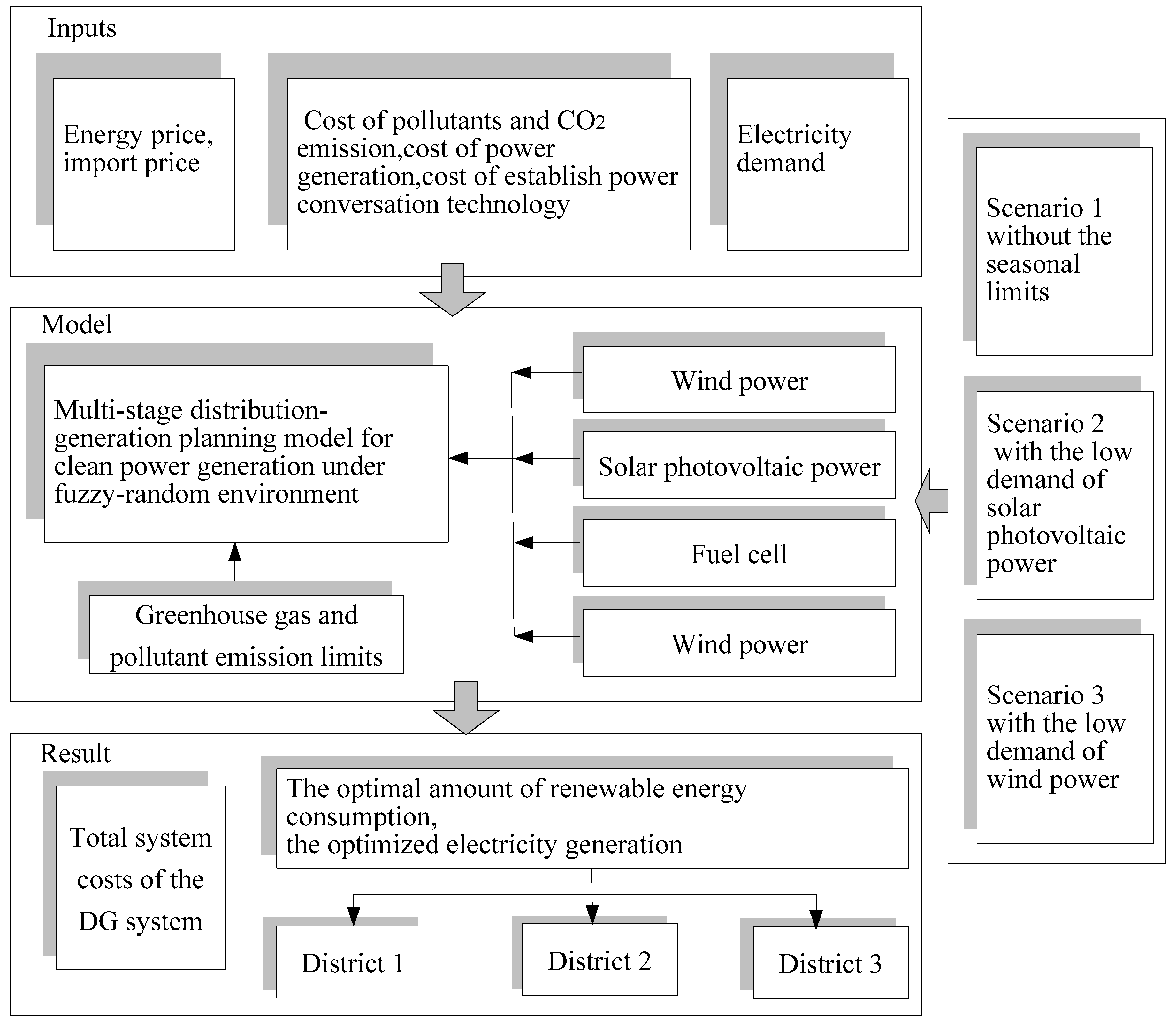
The flow chart of the model within the DG system is present in Figure 1.
3.3. Data Collection and Scenarios Definition
The planning horizon is 10 years (2006–2016) which is further divided into two periods with each representing a 5-year span. Related facilities are available for regional power generation. The related energy and economic data are obtained by analyzing representative reports of the studied area. According to Urumqi Statistics Bureau, the report of regional electric power group corporation, and electric power yearbook (from 2002 to 2014), the related data of regional electric power system demand are obtained, in which three discrete target values can be selected as fluctuate ranges (i.e., L, M and H). According to the data, the electricity demand in each district is shown in Table 1. Additionally, three scenarios are designed to reflect the effects of DG system structure, energy replacement potential, clean power generation, and the emission reduction targets. Scenario 1 represents the DG system without the seasonal limits, the technologies with strong seasonal restrictions would not be affected by the seasons (e.g., wind power and solar photovoltaic power). In this scenario, the uncertainties of wind power and solar photovoltaic power would be lower than other two scenarios. Then, the restraint conditions of wind power and solar photovoltaic power would be relieved in scenario 1. Scenario 2 represents a system with the low demand of solar photovoltaic power in winter with the solar photovoltaic generating capacity being limited by the sun radiation intensity and the temperature in winter. In this scenario, the uncertainties of solar photovoltaic power would be higher than other two scenarios. Therefore, the restraint conditions of solar photovoltaic power would be strengthened in scenario 2. Scenario 3 represents a system with the low demand of wind power in winter. The main reason would be the risk of wind speed and freeze in winter which would bring high instability to the power supply. The uncertainties of wind power would be higher than other two scenarios. Moreover, the restraint conditions of wind power would be strengthened in scenario 3.
4. Result and Discussion
The related economic and technical data of the system were acquired from reports of Urumqi Statistics Bureau and electric power yearbook. The optimized programming results for electric DG system programming are obtained from the MDGP model and would reveal the potentials and effects of energy replacement to regional electric system. Then, the analysis of results would explore the possibility of energy replacement in a DG system to meet regional power demands and emission reduction targets. Moreover, the solutions of the model would be expressed as intervals under different scenarios, which provide multiple alternatives to reflect the fluctuation of the response to variations in regional demands. On the other hand, the results describe that the patterns of regional DG system for power supply and demand would be relatively stable.
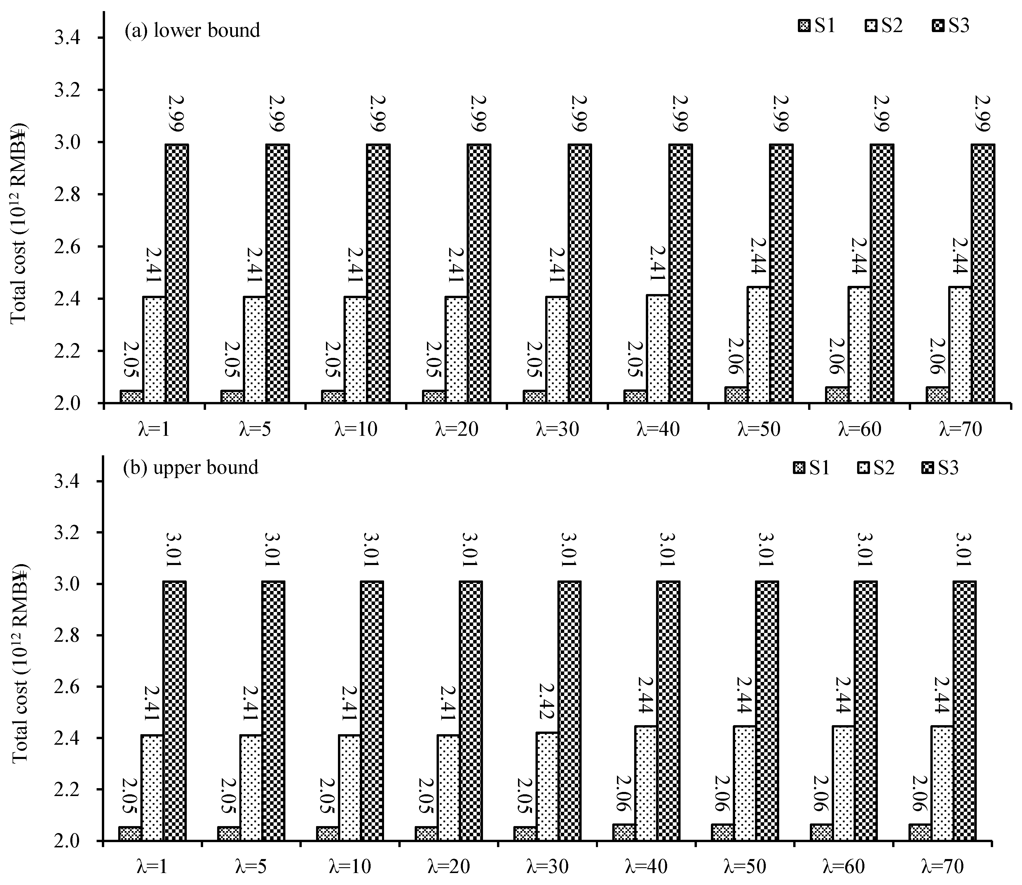
Figure 2 presents the total system costs of the DG system with two bounds under different scenarios. The net system cost has two extremes corresponding to different system conditions. The net cost of the DG system would increase as λ increases. The net cost would be RMB¥ [2.046, 2.052] × 1012, RMB¥ [2.046, 2.052] × 1012, RMB¥ [2.047, 2.052] × 1012, RMB¥ [2.060, 2.062] × 1012, RMB¥ [2.060, 2.062] × 1012 under scenario 1 with λ levels of 5, 10, 30, 50, 70, respectively. In the euro case, the net cost would be € [259.638, 260.399] × 109, € [259.638, 260.399] × 109, €[259.765, 260.399] × 109, € [261.415, 261.668] × 109, € [261.415, 261.668] × 109 under scenario 1 with λ levels of 5, 10, 30, 50, 70, respectively. In the dollar case, the net cost would be $ [298.896, 299.772] × 109, $ [298.896, 299.772] × 109, $ [299.042, 299.772] × 109, $ [300.941, 301.233] × 109, $ [300.941, 301.233] × 109 under scenario 1 with λ levels of 5, 10, 30, 50, 70, respectively. It reflects that the model possesses trade-off between system costs and stability. Then, failure risk of DG system would be lessened, and the decision feasibility would be enhanced as the λ increases. On the contrary, the risk would be higher, and the decision feasibility would be lower as the λ decreases. The results reflect that smaller costs may make higher failure risk and lower reliabilities. Higher system costs can guarantee lower system-failure risks and higher system reliabilities. Then, the decision-makers would face higher cost for more stable solution and lower cost for more variable solution. In addition, the total system cost would increase due to the expansion for scale of power replacement and renewable power generation. For example, with λ = 70, the cost would be RMB¥ [2.060, 2.062] × 1012, RMB¥ [2.444, 2.444] × 1012, and RMB¥ [2.989, 3.008] × 1012 under scenarios 1, 2, and 3, respectively. In the euro case, the net cost would be € [261.415, 261.668] × 109, € [309.983, 309.983] × 109, € [379.108, 381.716] × 109under scenarios 1, 2, and 3, respectively. In the dollar case, the net cost would be $ [300.941, 301.233] × 109, $ [357.101, 357.101] × 109, $ [436.733, 439.509] × 109 under scenarios 1, 2, and 3, respectively. Moreover, the scale of power replacement and renewable electric power generation would be limited by the regional geographical factors. The cost of DG system would have a slight variation by imported and exported electricity from power grid with traditional power generation.
The whole study area would be divided to 3 programming districts. Each district would choose an appropriate renewable energy power generation mode to constitute the DG system of Urumqi. The appropriate renewable energy power generation mode would be confirmedby the request and limit of economy, environment and geography in each district. From the solutions of the programming model, the districts 1–3 would choose the wind power, solar photovoltaic power, and natural gas turbine, respectively. In case of insufficient DG system electric supply, electricity would be imported at a high price from power grid. On the contrary, superfluous DG system electric supply would be exported to power grid.
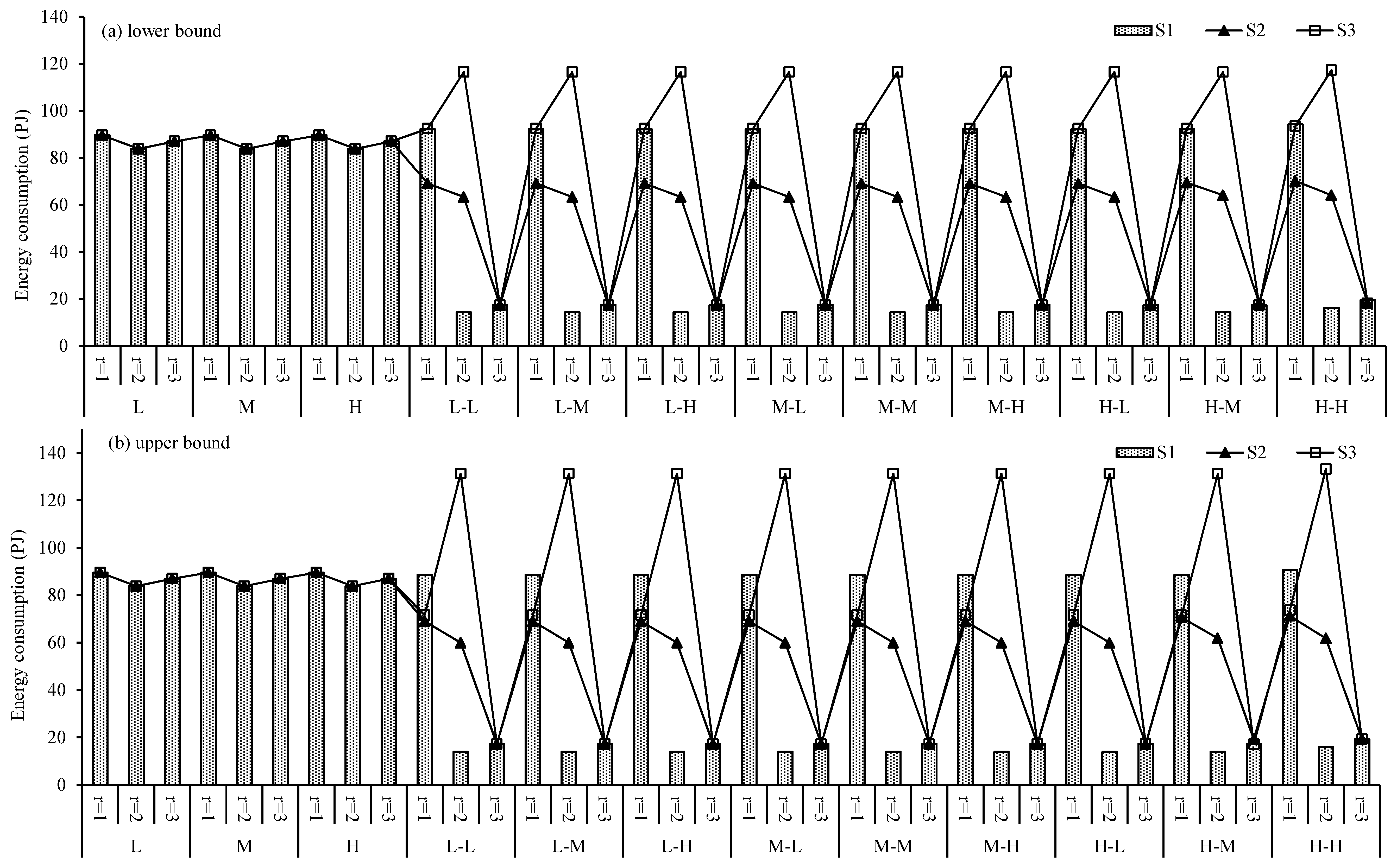
Figure 3 presents the optimal amount of renewable energy consumption for the DG system in each district. In the DG system of study area, a variety of techniques and renewable energy resources would compete for providing energies to different districts under various seasons and relevant district geography factors. The district 1 and district 2 would not have to pay the cost for energy purchases, due to the types of renewable energy resources of district 1 and district 2 (wind power for district 1 and solar photovoltaic power for district 2). In period 1, under lower bound, 89.54 PJ, 83.79 PJ and 86.98 PJ of pre-regular natural gas would be supplied to district 3 by domestic production and import. The results would correspond to the variations of the power generation in district 3. Then the variations of natural gas consumption under different power demand levels would be basically stable. For instance, in winter of period 2, under lower bound of scenario 3, the amount of natural gas consumption would be 116.53 PJ, 116.53 PJ, and 117.27 PJ under high-low (H-L) level, medium-high (M-L) level, and high-high (H-H) level, respectively. The amount of natural gas consumption would be 131.33 PJ, 131.33 PJ, and 133.20 PJ under high-low (H-L) level, medium-high (M-L) level, and high-high (H-H) level in winter of period 2 under upper bound of scenario 3, respectively. Although the amounts of pre-regular natural gas consumption in period 1 would have little variations from season 1 to season 3, the amount would have changes in season 2. It indicates that the natural gas consumption and power supply of district 3 would be sensitive in winter. The variations of natural gas consumption are mainly caused by the growth of regional power demands of district 3 and the price for power import from power grid.
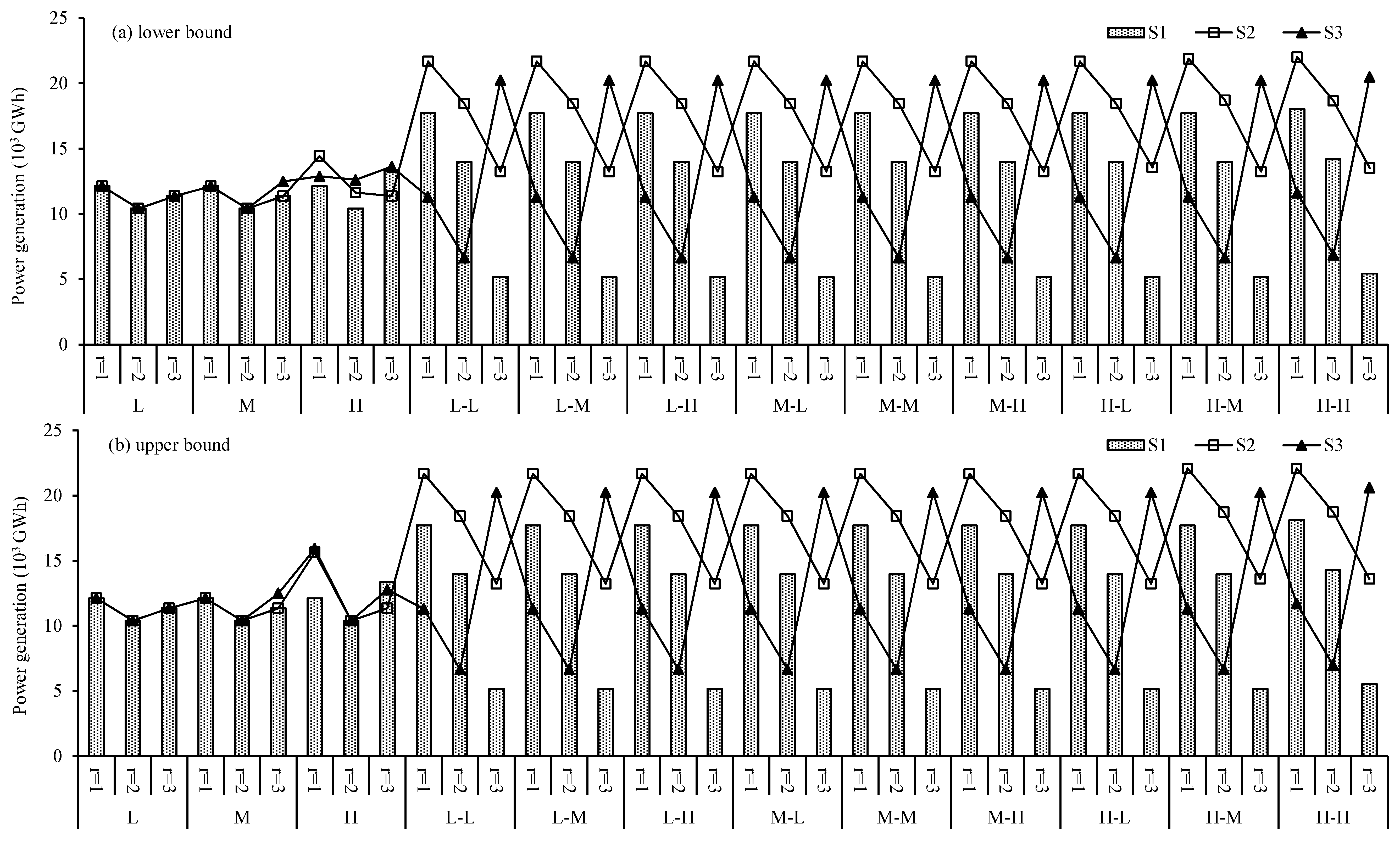
Figure 4, Figure 5 and Figure 6 show the optimized electricity generation in a conservative condition (λ = 70) for each district under varied scenarios. Although the renewable power generation in DG power system would vary as λ increases, the resulting power generation would increase stably. Then, power generation would be fixed when λ = 50, 60, 70. It indicates that the renewable power generation would increase as the stability of the regional DG power system is enhanced. Thus, the failure risk of DG power-structure adjustment would be lessened as λ values increase.
Generally, compared with the results with high robust criteria, the DG power generation would change as the variations of the district demand modes under different scenarios. In addition, Table 2, Table 3, Table 4, Table 5, Table 6 and Table 7 show the power generation in the condition of λ = 70 for each district under different scenarios and seasons. For instance, in winter of period 1 of district 1, under the high demand level, the DG electricity generation would be 12.12 × 10³ GWh, [14.41, 15.63] × 103 GWh, and [12.87, 15.91] × 103 GWh, in scenarios 1, 2, and 3, respectively; under H-M level (with the probability of 11%), it would be17.71 × 103 GWh, [21.86, 22.08] × 103 GWh, and 11.30 × 10³ GWh in all scenarios of period 2, respectively. Wind power, solar photovoltaic power, fuel cell, and natural gas turbine would be the main ways to generate clean electricity for DG power system in a regional power system. Due to the technology selection, geography factors, energy resources, and environmental risk limitations, fuel cells in Urumqi would be unsuitable for each district during the planning horizon. Then, the district 1, 2 and 3 would chose the wind power, solar photovoltaic power, and natural gas turbine as the power technology in the regional DG power system.
Figure 4, Table 2 and Table 3 show the optimized wind power generation schemes in district 1 under λ = 70. The district 1 includes Tianshan district, Shuimogou District, and Dabancheng District. The power generation schemes would show obvious seasonality. For example, wind power generation would be [18.01, 18.12] × 103 GWh, [14.19, 14.29] × 103 GWh, and [5.43, 5.52] × 103 GWh in season 1–3 of period 2 under the H-H demand level in scenarios 1. Based on the above analysis, the abundant wind sources in district 1 would provide stable base for wind power generation to DG system. Due to the technology, the capacity of wind power would be limited by wind speed. Then, the seasonality of wind speed and the power demand would determine the power generation under different seasons. On the other hand, wind power generation would be regular and stable under different regional develop modes (different scenarios). The power generation under different regional district develop modes would show obvious variations among each other. For example, under the high demand level, the pre-regulated wind power generation would be 12.12 × 10³ GWh, 14.41 × 10³ GWh, and 12.86 × 10³ GWh under scenarios 1, 2 and 3 in summer of period 1. Then, in summer of period 2, the optimized electricity generation would be [18.02, 18.12] × 103 GWh, [21.98, 22.09] × 103 GWh, and [11.61, 11.71] × 103 GWh in scenarios 1, 2, and 3 under the H-H demand level. From Figure 4, the electricity generation of scenario 3 would have a variation in season 2. The main reason would be that the wind speed of season 2 and season 3 has low and high stability, respectively. In the contrary, electricity generation stability of scenarios 1 and 2 would be reduced due to the power demand of different season. Therefore, the targets of different scenarios would impact the power generation of DG system greatly.
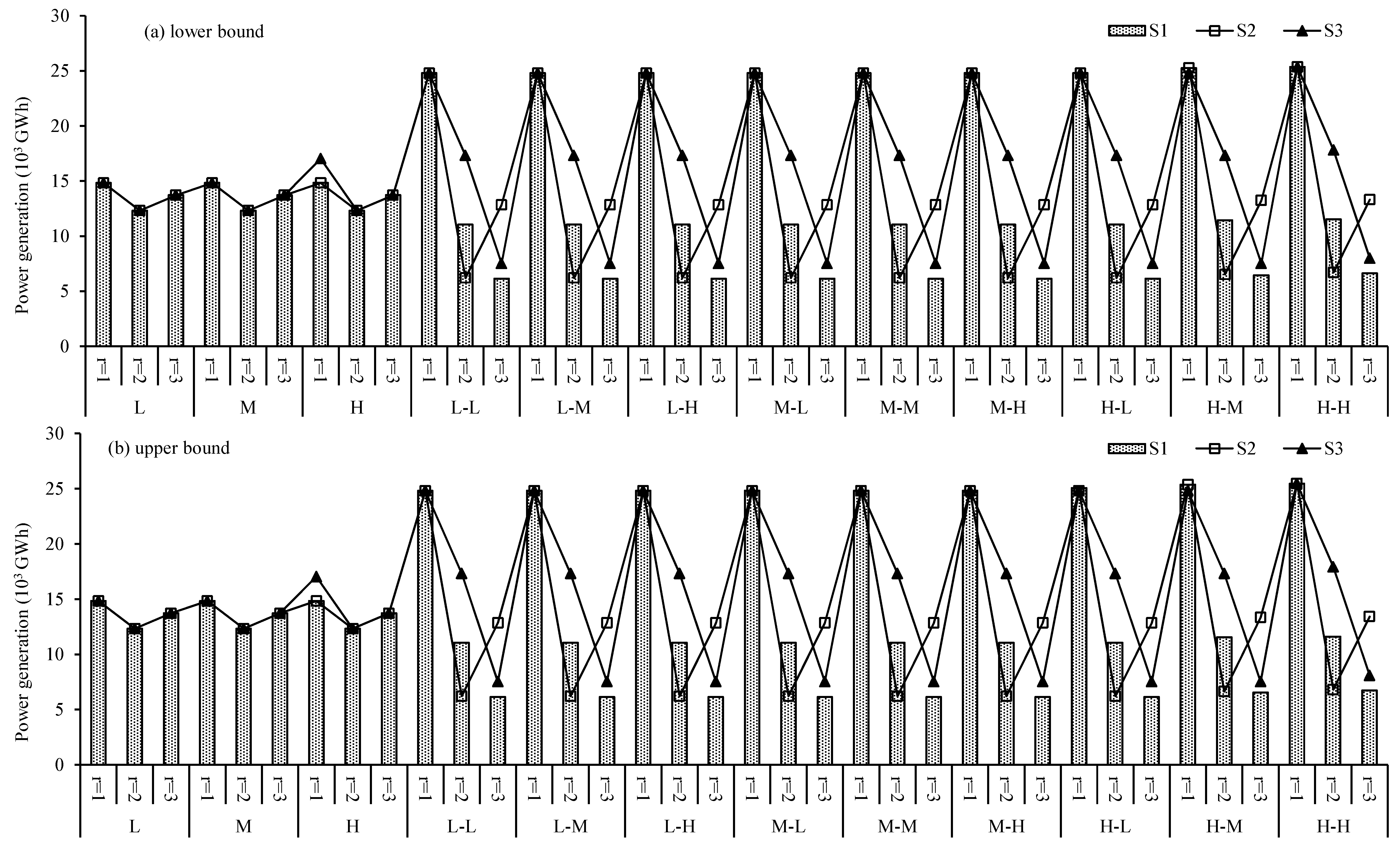
Figure 5, Table 4 and Table 5 show the optimized solar photovoltaic power generation schemes in district 2 under the λ = 70. The district 2 includes Saybagh District, Xinshi District, Toutunhe District, and Urumqi County. The solar photovoltaic power would be chosen to get maximum electricity supply security in DG power system of district 2. The solar photovoltaic power generation schemes would also show obvious seasonality like the wind power in district 1. For example, under the H-H demand level of scenarios 3, solar photovoltaic power generation would be [25.36, 25.46] × 103 GWh, [17.81, 17.92] × 103 GWh, and [7.99, 8.09] × 103 GWh in season 1, 2 and 3 of period 2. Though the stability of the solar photovoltaic power technology has been improved, the power generation would be affected by different seasons. The main reason would be the seasonality of the solar photovoltaic source. The solar photovoltaic power capacity would be limited by the sun radiation intensity and the temperature. Then, the obvious seasonality and the power demand of each season would affect the power generation under different seasons. On the other hand, power generation would have different variations under different regional district develop modes (different scenarios). Along with the development of solar photovoltaic technology, the solar generation targets in scenarios 2 would be more mutative than in scenarios 1 and 3 under different season. For instance, under scenario 2, in period 2, the optimized electricity generation would be [25.36, 25.46] × 103 GWh, [6.71, 6.81] × 103 GWh, and [13.32, 13.43] × 103 GWh in H-Hdemand level. The electricity generation would be [25.36, 25.46] × 103 GWh, [17.82, 17.91] × 103 GWh, and [7.99, 8.09] × 103 GWh in H-H demand level of period 2 under scenario 3. The electricity generation would have an insignificant change in season 2 under scenario 2. The main reason would be the sun radiation intensity and the temperature in season 2. The sun radiation intensity of season 2 has low stability, and the temperature would be lower in season 2 than others. In the contrary, electricity generation of scenario 1 and 3 would reduce stably due to the power demand of different season. It indicated that different modes would impact the power generation of DG system.
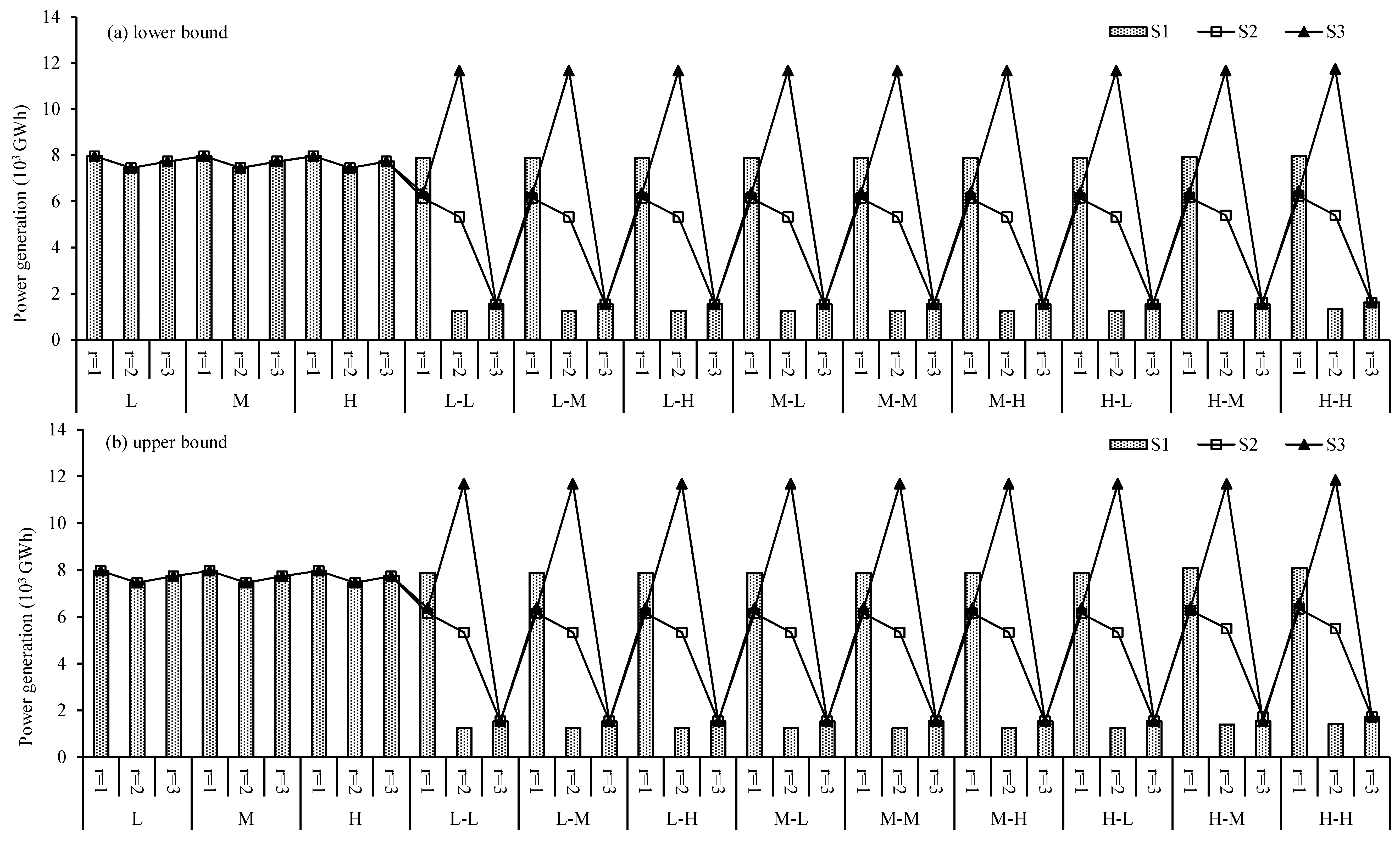
Figure 6, Table 6 and Table 7 show the optimized natural gas turbine power generation schemes in district 3 under the λ = 70. The main area of district 3 includes Midong District. The geographical factor of Midong District leads to inappropriate choice for the wind and solar photovoltaic power. The stability of wind and solar photovoltaic power in district 3 would not satisfy the system requirement and security. Moreover, the net cost of fuel cell power for district 3 would be higher than the net cost of natural gas turbine power. The natural gas turbine power would be reasonable under different scenarios. The power generation of scenario 3 would be [6.45, 6.56] × 103 GWh, [11.74, 11.83] × 103 GWh, and [1.61, 1.72] × 103 GWh under the H-H demand level in period 2. The power generation of scenario 2 would be [6.23, 6.33] × 103 GWh, [5.39, 5.50] × 103 GWh, and [1.61, 1.72] × 103 GWh under the H-H demand level in period 2. The power generation of scenario 1 would be [7.97, 8.08] × 103 GWh, [1.31, 1.42] × 103 GWh, and [1.61, 1.71] × 103 GWh under the H-H demand level in period 2. Although the optimal electricity consumption would have great difference, the generation would show the basic property of different scenarios. In addition, the result shows that the DG system has great flexibility ratio in the regional power replacement of renewable energy.
The renewable resource computation would bring very little emission. Then, the optimized results of power generation schemes would meet both regional energy system demand and emission reduction target. On the other hand, the abundant sustainable power resources of Urumqi provide great potentials for renewable power development. Therefore, Urumqi has the capacity to practice the renewable energy replacement with DG power system. To improve usage and capacity of green power generation, the decision-makers and planners would play driving roles to create more demonstration projects for promoting the development of regional renewable power system. The DG power system can also lead to a stable power pattern with substantial clean electricity. The solutions from MDGP can support decisions of renewable energy replacement, and pollutant emissions reduce under different district demand modes. The multiple solutions are effective to represent various options reflecting regional DG power system and environmental-economic tradeoffs.
5. Conclusions
In this research, a MDGP model was developed for clean power generation in a regional DG power system under multiple uncertainties. Methods of FRIP, SRO, and MSP were incorporated into the MDGP model. The integration of FRIP, SRO, and MSP has a special meaning for reflecting compound uncertainties in DG power systems. The original model would provide an effective linkage among renewable energy replacement, seasonal impact factors, and the district demand modes. The developed model could also help analyze the trade-off between system cost, stability and the associated risk-aversion levels. The obtained solutions under different district demand modes and seasons could help get multiple decision alternatives.
The developed model was applied to a DG power system in Urumqi, China. Three scenarios and three districts are designed based on district demand modes, seasonal feature, and clean power generation, receptively. The net system cost, imported electricity, and clean power generation schemes were analyzed. Each scenario corresponded to specific weather limits of renewable energy technology and power demand level. Results reflected that different weather limits and power demand levels would correspond to different DG power generation schemes. Traditional power generation would be replaced by renewable energy power to improve regional power structure, and environmental protection requests. The replacement of a DG system would make an important contribution to relieving energy and environmental stress. Traditional power generation would be decreased with the improvement of energy structure adjustment in Urumqi. On the other hand, Urumqi has unique strength in renewable energy. Therefore, the development of renewable energy power could be a major direction for the Urumqi power system. The development of grid-connected renewable power generation would be realized over the next few years.
This research could help regional power system planners to identify DG power management and discuss the potential of clean energy substitution in Urumqi under various weather limits, district demand modes, risk and economic considerations. However, there are still several limitations in this research. Firstly, more energy factors of the system may be considered to obtain detailed power generation schemes. The technical constraints such as voltage limits, ampacity level of the network’s branches and the possibility of reverse power flow would be interesting topics that deserve future research efforts. Moreover, the power load demands, environmental requirements and regional management patterns are obviously impacted by the energy policy. Therefore, further studies are desired to solve practical problems in regional power systems.
Author Contributions
Conceptualization, G.H. and Y.F.; Data curation, S.W.; Formal analysis, S.W.; Funding acquisition, G.H.; Investigation, S.W.; Methodology, S.W. and Y.F.; Resources, Y.F.; Software, S.W.; Supervision, G.H.; Validation, S.W.; Visualization, S.W.; Writing—original draft, S.W.; Writing—review & editing, S.W. and Y.F.
Funding
This research received no external funding.
Acknowledgments
This research was supported by the National Key Research and Development Plan (2016YFC0502800, 2016YFA0601502), the Natural Sciences Foundation (51520105013, 51679087), the 111 Program (B14008) and the Natural Science and Engineering Research Council of Canada.
Conflicts of Interest
The authors declare no conflict of interest.
Appendix A. Solving Method
There are a variety of uncertainties existing in power systems. Accordingly, effectively dealing with uncertainties is of significance to regional planners. Fuzzy sets, probability distributions, and multiple uncertainties are familiar uncertainties. Fuzzy sets can be expressed as with membership function , representing an approximate interval with possible distributions. Then, the fuzzy sets can be applied for reflecting uncertainties which can be expressed as intervals with core subjects to feasible possible distributions. For uncertain parameters in power system problems, simplex intervals may lead to oversimplification at a certain degree, resulting in the loss of information. Then, fuzzy sets can remedy this shortage. Probability distributions can be expressed as with a distribution function . Energy prices over a specific period and scenario can be expressed as probability distributions based on historical records and a literature review. Multiple uncertainties are combinations of dual or more uncertainties. For instance, when estimating the lower and upper bounds of interval parameters, different subjective judgments would be made by different decision-makers. Then, this phenomenon leads to a variety of fuzzy sets subject to certain probability distribution, representing multiple uncertainties. Such uncertainties can be described as fuzzy-random variables.
The model would be transformed as follows:
Subject to:
where is slack variable. The constraint with slack variable is the specific control constraint. The solving method of multistage fuzzy-random inexact stochastic programming would be developed to imply in the robust programming. Then, the solving method would be introduced as follow:
Firstly, family of triangular fuzzy numbers () can be defined as follows:
and
where and () are the left and right spreads, respectively. The triangular fuzzy set can be illustrated as . Then, measuring superiority and inferiority degrees of the function can be a method for comparing fuzzy. Beginning with the levels of two fuzzy sets ( and ) as:
If , then .
Therefore, the area difference of and represent the superiority between and . Mathematically, the area can be presented as follows:
Thus, superiority between and can be defined as (e.g., superiority of over )
Analogously, the inferiority of to is
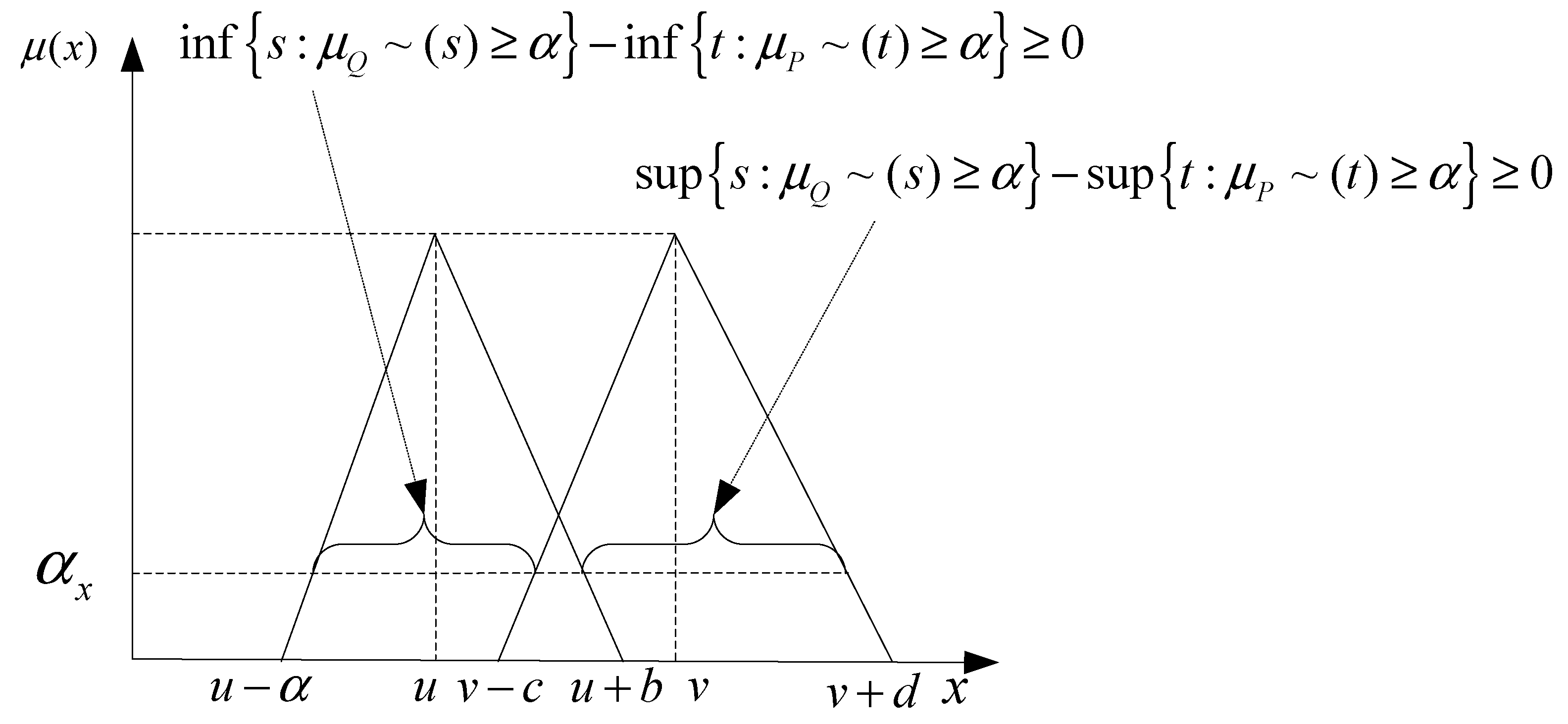
Consider triangular fuzzy sets and , where , the superiority of over and the inferiority of to can be quantified as
Figure A1.
Superiority and inferiority between and at a-cut level.

This method can be applied to measure the superiority and inferiority between fuzzy-random variables. A fuzzy-random variable on the space is a fuzzy set-valued mapping as follows:
Then, the Borel set (B) under a cut level:
Secondly, for two triangular fuzzy-random variables , the superiority of fuzzy-random variable over and inferiority of fuzzy-random variable to are
The above method for measuring superiority and inferiority can be used to solve FRIP problems with fuzzy-stochastic coefficients. Then, FRIP method can be presented as follows:
Subject to:
where , , , , denotes a set of interval numbers with fuzzy-random boundaries, denotes a set of interval numbers. Then, solutions of FRIP can be obtained through two steps. The second sub-model () can be obtained based on the solution of the formulated first sub-model () (when the objective function is to be minimized). In detail, the first sub-model can be formulated as follows:
subject to:
where are interval variables of objective function which are with positive coefficients, and are interval variables of objective function which are with negative coefficients, = the probability level. This sub-model can be transformed into:
subject to
Then, the above model can be transformed into
subject to
Solutions of and can be obtained through solving sub-model with . Then, another sub-model with can be formulated as follows (assume that , and ):
subject to
Thus, the above model can be transformed into
Hence, solutions of and can be obtained from sub-model. and as final solution for model can then be obtained. These solutions with interval form can be further interpreted for generating multiple schemes and decision alternatives.
References
- Cristóbal, J.; Guillén-Gosálbez, G.; Jiménez, L.; Irabien, A. Multi-objective optimization of coal-fired electricity production with CO2, capture. Appl. Energy 2012, 98, 266–272. [Google Scholar] [CrossRef]
- Dubreuil, A.; Assoumou, E.; Bouckaert, S.; Selosse, S.; Maı¨zi, N. Water modeling in an energy optimization framework—The water-scarce middle east context. Appl. Energy 2013, 101, 268–279. [Google Scholar] [CrossRef]
- Porkar, S.; Poure, P.; Abbaspour-Tehrani-Fard, A.; Saadate, S. A novel optimal distribution system planning framework implementing distributed generation in a deregulated electricity market. Electr. Power Syst. Res. 2010, 80, 828–837. [Google Scholar] [CrossRef]
- Haghifam, M.R.; Falaghi, H.; Malik, O.P. Risk-based distributed generation placement. IET Gener. Transm. Distrib. 2008, 2, 252–260. [Google Scholar] [CrossRef]
- Sajjadi, S.M.; Haghifam, M.R.; Salehi, J. Simultaneous placement of distributed generation and capacitors in distribution networks considering voltage stability index. Int. J. Electr. Power Energy Syst. 2013, 46, 366–375. [Google Scholar] [CrossRef]
- Cha, J.H.; Park, K.W.; Ahn, H.S.; Kwon, K.M.; Oh, J.H.; Mahirane, P.; Kim, J.E. Overvoltage Protection Controller Design of Distributed Generation Connected to Power Grid Considering Islanding Condition. J. Electr. Eng. Technol. 2018, 13, 599–607. [Google Scholar]
- Su, H.; Zhang, Z. Power Flow Algorithm for Weakly Meshed Distribution Network with Distributed Generation Based on Loop-analysis in Different Load Models. J. Electr. Eng. Technol. 2018, 13, 608–619. [Google Scholar]
- Arcos-Aviles, D.; Pascual, J.; Guinjoan, F.; Marroyo, L.; Sanchis, P.; Marietta, M.P. Low complexity energy management strategy for grid profile smoothing of a residential grid-connected microgrid using generation and demand forecasting. Appl. Energy 2017, 205, 69–84. [Google Scholar] [CrossRef]
- Hu, Q. Planning of Electric Power Generation Systems under Multiple Uncertainties and Constraint-Violation Levels. J. Environ. Inform. 2014, 23, 55–64. [Google Scholar] [CrossRef] [Green Version]
- Fan, Y.R.; Huang, G.H.; Baetz, B.W.; Li, Y.P.; Huang, K. Development of a Copula-based Particle Filter (CopPF) Approach for Hydrologic Data Assimilation under Consideration of Parameter Interdependence. Water Resour. Res. 2017, 53, 4850–4875. [Google Scholar] [CrossRef]
- Fan, Y.R.; Huang, G.H.; Veawab, A. A generalized fuzzy linear programming approach for environmental management problem under uncertainty. J. Air Waste Manag. Assoc. 2012, 62, 72–86. [Google Scholar] [CrossRef] [PubMed]
- Hu, Q.; Huang, G.; Fan, Y.; Liu, Z.; Li, W. Inexact fuzzy two-stage programming for water resources management in an environment of fuzziness and randomness. Stoch. Environ. Res. Risk Assess. 2012, 26, 261–280. [Google Scholar] [CrossRef]
- Fan, Y.R.; Huang, G.H.; Huang, K.; Baetz, B.W. Planning Water Resources Allocation Under Multiple Uncertainties Through a Generalized Fuzzy Two-Stage Stochastic Programming Method. IEEE Trans. Fuzzy Syst. 2015, 23, 1488–1504. [Google Scholar] [CrossRef]
- Wang, K.; Zhang, X.; Wei, Y.-M.; Yu, S. Regional allocation of CO2 emissions allowance over provinces in China by 2020. Energy Policy 2013, 54, 214–229. [Google Scholar] [CrossRef]
- Cai, Y.P.; Huang, G.H.; Yang, Z.F.; Lin, Q.G.; Bass, B.; Tan, Q. Development of an optimization model for energy systems planning in the Region of Waterloo. Int. J. Energy Res. 2008, 32, 988–1005. [Google Scholar] [CrossRef]
- Cheng, G.; Huang, G.H.; Dong, C. Interval Recourse Linear Programming for Resources and Environmental Systems Management under Uncertainty. J. Environ. Inform. 2017, 30, 119–136. [Google Scholar] [CrossRef]
- Babacan, O.; Ratnam, E.L.; Disfani, V.R.; Kleissl, J. Distributed energy storage system scheduling considering tariff structure, energy arbitrage and solar PV penetration. Appl. Energy 2017, 205, 1384–1393. [Google Scholar] [CrossRef]
- Li, Y.; Li, Y.; Ji, P.; Yang, J. Development of energy storage industry in China: A technical and economic point of review. Renew. Sustain. Energy Rev. 2015, 49, 805–812. [Google Scholar] [CrossRef]
- Diab, S.; Gerogiorgis, D.I. Process modelling, simulation and technoeconomic eva luation of crystallisation antisolvents for the continuous pharmaceutical manu facturing of rufinamide. Comput. Chem. Eng. 2018, 111, 102–114. [Google Scholar] [CrossRef]
- Cai, Y.; Huang, G.H.; Nie, X.H.; Li, Y.P.; Tan, Q. Municipal Solid Waste Management Under Uncertainty: A Mixed Interval Parameter Fuzzy-Stochastic Robust Programming Approach. Environ. Eng. Sci. 2007, 24, 338–352. [Google Scholar] [CrossRef]
- Desjardins, R.; Worth, D.; Vergé, X.; Maxime, D.; Dyer, J.; Cerkowniak, D. Carbon Footprint of Beef Cattle. Sustainability 2012, 4, 3279–3301. [Google Scholar] [CrossRef] [Green Version]
- Huang, C.Z.; Nie, S.; Guo, L.; Fan, Y.R. Inexact Fuzzy Stochastic Chance Constraint Programming for Emergency Evacuation in Qinshan Nuclear Power Plant under Uncertainty. J. Environ. Inform. 2017, 30, 63–78. [Google Scholar] [CrossRef]
- Cai, Y.P.; Huang, G.H.; Tan, Q. An inexact optimization model for regional energy systems planning in the mixed stochastic and fuzzy environment. Int. J. Energy Res. 2009, 33, 443–468. [Google Scholar] [CrossRef]
- Christian, B.; Cremaschi, S. A Multistage Stochastic Programming Formulation to Evaluate Feedstock/Process Development for the Chemical Process Industry. Chem. Eng. Sci. 2018, 187, 223–244. [Google Scholar] [CrossRef]
- Tham, C.K.; Cao, B. Stochastic Programming Methods for Workload Assignment in an Ad Hoc Mobile Cloud. IEEE Trans. Mob. Comput. 2017, 17, 1709–1722. [Google Scholar] [CrossRef]
- Katagiri, H.; Kato, K.; Uno, T. Possibility/Necessity-Based Probabilistic Expectation Models for Linear Programming Problems with Discrete Fuzzy Random Variables. Symmetry 2017, 9, 254. [Google Scholar] [CrossRef]
- Bootaki, B.; Mahdavi, I.; Paydar, M.M. New bi-objective robust design-based utilisation towards dynamic cell formation problem with fuzzy random demands. Int. J. Comput. Integr. Manuf. 2015, 28, 577–592. [Google Scholar] [CrossRef]
- Xu, J.; Ma, Y.; Xu, Z. A Bilevel Model for Project Scheduling in a Fuzzy Random Environment. IEEE Trans. Syst. Man Cybern. Syst. 2015, 45, 1322–1335. [Google Scholar] [CrossRef]
- Calinescu, R.; Češka, M.; Gerasimou, S.; Kwiatkowska, M.; Paoletti, N. Efficient Synthesis of Robust Models for Stochastic Systems. J. Syst. Softw. 2018, 143, 140–158. [Google Scholar] [CrossRef]
- Li, Y.; Lu, J.; Kou, C.; Mao, X.; Pan, J. Robust discrete-state-feedback stabilization of hybrid stochastic systems with time-varying delay based on Razumikhin technique. Stat. Probab. Lett. 2018, 139, 152–161. [Google Scholar] [CrossRef]
- Fazlikhalaf, M.; Mirzazadeh, A.; Pishvaee, M.S. A robust fuzzy stochastic programming model for the design of a reliable green closed-loop supply chain network. Hum. Ecol. Risk Assess. 2017, 23, 2119–2149. [Google Scholar] [CrossRef]
- Ishak, A.B. Variable Selection Based on Statistical Learning Approaches to Improve PM10 Concentration Forecasting. J. Environ. Inform. 2016, 30, 79–94. [Google Scholar]
- Xiong, C.; Yang, D.; Huo, J. Spatial-Temporal Characteristics and LMDI-Based Impact Factor Decomposition of Agricultural Carbon Emissions in Hotan Prefecture, China. Sustainability 2016, 8, 262. [Google Scholar] [CrossRef]
- Guo, L.; Li, Y.P.; Huang, G.H.; Wang, X.W.; Cai, C. Development of an Interval-Based Evacuation Management Model in Response to Nuclear-Power Plant Accident. J. Environ. Inform. 2012, 20, 58–66. [Google Scholar] [CrossRef] [Green Version]
- Nocca, F. The Role of Cultural Heritage in Sustainable Development: Multidimensional Indicators as Decision-Making Tool. Sustainability 2017, 9, 1882. [Google Scholar] [CrossRef]
- Suo, M.Q. Electric Power System Planning under Uncertainty Using Inexact Inventory Nonlinear Programming Method. J. Environ. Inform. 2013, 22, 49–67. [Google Scholar] [CrossRef] [Green Version]
- Bennetzen, E.H.; Smith, P.; Porter, J.R. Decoupling of greenhouse gas emissions from global agricultural production: 1970–2050. Glob. Chang. Biol. 2016, 22, 763–781. [Google Scholar] [CrossRef] [PubMed]
- Huang, G.H. Ipwm: An Interval Parameter Water Quality Management Model. Eng. Optim. 1996, 26, 79–103. [Google Scholar] [CrossRef]
- Huang, K.; Dai, L.M.; Yao, M.; Fan, Y.R.; Kong, X.M. Modelling Dependence between Traffic Noise and Traffic Flow through An Entropy-Copula Method. J. Environ. Inform. 2017, 29, 134–151. [Google Scholar] [CrossRef]
- Mohseni-Bonab, S.M.; Rabiee, A. Optimal reactive power dispatch: A review, and a new stochastic voltage stability constrained multi-objective model at the presence of uncertain wind power generation. IET Gener. Transm. Distrib. 2017, 11, 815–829. [Google Scholar] [CrossRef]
- Sahu, R.K.; Panda, S.; Yegireddy, N.K. A novel hybrid DEPS optimized fuzzy PI/PID controller for load frequency control of multi-area interconnected power systems. J. Process Control 2014, 24, 1596–1608. [Google Scholar] [CrossRef]
- Li, Y.P.; Nie, S.; Huang, C.Z.; McBean, E.A.; Fan, Y.R.; Huang, G.H. An integrated risk analysis method for planning water resource systems to support sustainable development of an arid region. J. Environ. Inform. 2017, 29, 1–15. [Google Scholar] [CrossRef]
- Al-Maliki, W.A.K.; Alobaid, F.; Kez, V.; Epple, B. Modelling and dynamic simulation of a parabolic trough power plant. J. Process Control 2016, 39, 123–138. [Google Scholar] [CrossRef]
- Sardou, I.G.; Zare, M.; Azad-Farsani, E. Robust energy management of a microgrid with photovoltaic inverters in VAR compensation mode. Int. J. Electr. Power Energy Syst. 2018, 98, 118–132. [Google Scholar] [CrossRef]
- Pastori, M.; Udias, A.; Bouraoui, F.; Bidoglio, G. A Multi-Objective Approach to Evaluate the Economic and Environmental Impacts of Alternative Water and Nutrient Management Strategies in Africa. J. Environ. Inform. 2017, 29, 16–28. [Google Scholar] [CrossRef]
Figure 1.
Flow chart of the multistage distribution-generation planning model for clean power generation.
Figure 1.
Flow chart of the multistage distribution-generation planning model for clean power generation.

Figure 2.
System cost under different scenarios. (a) Lower bound for result; (b) Upper bound for result.
Figure 2.
System cost under different scenarios. (a) Lower bound for result; (b) Upper bound for result.

Figure 3.
Optimized natural gas consumption in district 3 under different scenarios. (a) Lower bound for result; (b) Upper bound for result.
Figure 3.
Optimized natural gas consumption in district 3 under different scenarios. (a) Lower bound for result; (b) Upper bound for result.

Figure 4.
Optimized wind power generation in district 1 under different scenarios. (a) Lower bound for result; (b) Upper bound for result.
Figure 4.
Optimized wind power generation in district 1 under different scenarios. (a) Lower bound for result; (b) Upper bound for result.

Figure 5.
Optimized solar photovoltaic power generation in district 2 under different scenarios. (a) Lower bound for result; (b) Upper bound for result.
Figure 5.
Optimized solar photovoltaic power generation in district 2 under different scenarios. (a) Lower bound for result; (b) Upper bound for result.

Figure 6.
Optimized natural gas turbine power generation in district 3 under different scenarios. (a) Lower bound for result; (b) Upper bound for result.
Figure 6.
Optimized natural gas turbine power generation in district 3 under different scenarios. (a) Lower bound for result; (b) Upper bound for result.


Table 1.
Power demand of each district.
| Period | Demand Sequence (Probability %) | Power Demand (103 GWh) | ||
|---|---|---|---|---|
| District 1 | District 2 | District 3 | ||
| t = 1 | L (25) | 74.64 | 75.91 | 85.86 |
| M (35) | 81.48 | 83.02 | 95.18 | |
| H (40) | 85.53 | 87.04 | 102.86 | |
| t = 2 | L-L (6.25) | 72.64 | 72.64 | 76.86 |
| L-M (8.75) | 76.64 | 75.32 | 80.86 | |
| L-H (10) | 76.94 | 75.59 | 84.86 | |
| M-L (8.75) | 79.48 | 84.20 | 89.18 | |
| M-M (12.25) | 83.48 | 87.46 | 90.58 | |
| M-H (14) | 85.98 | 87.79 | 94.18 | |
| H-L (10) | 87.53 | 108.73 | 102.26 | |
| H-M (14) | 90.93 | 113.22 | 105.86 | |
| H-H (16) | 92.93 | 113.67 | 110.86 | |
Table 2.
Solution of power generation under λ = 70 in district 1 during the period 1.
| Season | Demand Sequence | Probability (%) | Optimized Generation Quantity (103 GWh) | ||
|---|---|---|---|---|---|
| Scenario 1 | Scenario 2 | Scenario 3 | |||
| Season 1 (summer) | L | 25 | 12.12 | 12.12 | 12.12 |
| M | 35 | 12.12 | 12.12 | 12.12 | |
| H | 40 | 12.12 | [14.41, 15.63] | [12.86, 15.91] | |
| Season 2 (winter) | L | 25 | 10.40 | 10.40 | 10.40 |
| M | 35 | 10.40 | 10.40 | 10.40 | |
| H | 40 | 10.40 | [10.40, 11.62] | [10.40, 12.61] | |
| Season 3 (transition season) | L | 25 | 11.35 | 11.35 | 11.35 |
| M | 35 | 11.35 | 11.35 | 12.48 | |
| H | 40 | 13.37 | 11.35 | [12.77, 13.61] | |
Table 3.
Solution of power generation under λ = 70 in district 1 during the period 2.
| Season | Demand Sequence | Probability (%) | Optimized Generation Quantity (103 GWh) | ||
|---|---|---|---|---|---|
| Scenario 1 | Scenario 2 | Scenario 3 | |||
| Season 1 (summer) | L-L | 6.25 | 17.71 | 21.67 | 11.30 |
| L-M | 8.75 | 17.71 | 21.67 | 11.30 | |
| L-H | 10 | 17.71 | 21.67 | 11.30 | |
| M-L | 8.75 | 17.71 | 21.67 | 11.30 | |
| M-M | 12.25 | 17.71 | 21.67 | 11.30 | |
| M-H | 14 | 17.71 | 21.67 | 11.30 | |
| H-L | 10 | 17.71 | 21.67 | 11.30 | |
| H-M | 14 | 17.71 | [21.86, 22.08] | 11.30 | |
| H-H | 16 | [18.01, 18.12] | [21.99, 22.09] | [11.61, 11.71] | |
| Season 2 (winter) | L-L | 6.25 | 13.96 | 18.43 | 6.65 |
| L-M | 8.75 | 13.96 | 18.43 | 6.65 | |
| L-H | 10 | 13.96 | 18.43 | 6.65 | |
| M-L | 8.75 | 13.96 | 18.43 | 6.65 | |
| M-M | 12.25 | 13.96 | 18.43 | 6.65 | |
| M-H | 14 | 13.96 | 18.43 | 6.65 | |
| H-L | 10 | 13.96 | 18.43 | 6.65 | |
| H-M | 14 | 13.96 | [18.70, 18.72] | 6.65 | |
| H-H | 16 | [14.19, 14.29] | [18.65, 18.75] | [6.87, 6.97] | |
| Season 3 (transition season) | L-L | 6.25 | 5.15 | 13.23 | 20.23 |
| L-M | 8.75 | 5.15 | 13.23 | 20.23 | |
| L-H | 10 | 5.15 | 13.23 | 20.23 | |
| M-L | 8.75 | 5.15 | 13.23 | 20.23 | |
| M-M | 12.25 | 5.15 | 13.23 | 20.23 | |
| M-H | 14 | 5.15 | 13.23 | 20.23 | |
| H-L | 10 | 5.15 | [13.23, 13.54] | 20.23 | |
| H-M | 14 | 5.15 | 13.23 | 20.23 | |
| H-H | 16 | [5.43, 5.52] | [13.50, 13.60] | [20.50, 20.60] | |
Table 4.
Solution of power generation under λ = 70 in district 2 during the period 1.
| Season | Demand Sequence | Probability (%) | Optimized Generation Quantity (103 GWh) | ||
|---|---|---|---|---|---|
| Scenario 1 | Scenario 2 | Scenario 3 | |||
| Season 1 (summer) | L | 25 | 14.83 | 14.83 | 14.83 |
| M | 35 | 14.83 | 14.83 | 14.83 | |
| H | 40 | 14.83 | 14.83 | 17.04 | |
| Season 2 (winter) | L | 25 | 12.33 | 12.33 | 12.33 |
| M | 35 | 12.33 | 12.33 | 12.33 | |
| H | 40 | 12.33 | 12.33 | 12.33 | |
| Season 3 (transition season) | L | 25 | 13.72 | 13.72 | 13.72 |
| M | 35 | 13.72 | 13.72 | 13.72 | |
| H | 40 | 13.72 | 13.72 | 13.72 | |
Table 5.
Solution of power generation under λ = 70 in district 2 during the period 2.
| Season | Demand Sequence | Probability (%) | Optimized Generation Quantity (103 GWh) | ||
|---|---|---|---|---|---|
| Scenario 1 | Scenario 2 | Scenario 3 | |||
| Season 1 (summer) | L-L | 6.25 | 24.81 | 24.81 | 24.81 |
| L-M | 8.75 | 24.81 | 24.81 | 24.81 | |
| L-H | 10 | 24.81 | 24.81 | 24.81 | |
| M-L | 8.75 | 24.81 | 24.81 | 24.81 | |
| M-M | 12.25 | 24.81 | 24.81 | 24.81 | |
| M-H | 14 | 24.81 | 24.81 | 24.81 | |
| H-L | 10 | [24.81, 25.07] | 24.81 | 24.81 | |
| H-M | 14 | [25.26, 25.36] | [25.26, 25.36] | 24.81 | |
| H-H | 16 | [25.36, 25.46] | [25.36, 25.46] | [25.36, 25.46] | |
| Season 2 (winter) | L-L | 6.25 | 11.04 | 6.21 | 17.32 |
| L-M | 8.75 | 11.04 | 6.21 | 17.32 | |
| L-H | 10 | 11.04 | 6.21 | 17.32 | |
| M-L | 8.75 | 11.04 | 6.21 | 17.32 | |
| M-M | 12.25 | 11.04 | 6.21 | 17.32 | |
| M-H | 14 | 11.04 | 6.21 | 17.32 | |
| H-L | 10 | 11.04 | 6.21 | 17.32 | |
| H-M | 14 | [11.44, 11.54] | [6.53, 6.63] | 17.32 | |
| H-H | 16 | [11.51, 11.61] | [6.71, 6.81] | [17.82, 17.91] | |
| Season 3 (transition season) | L-L | 6.25 | 6.13 | 12.85 | 7.52 |
| L-M | 8.75 | 6.13 | 12.85 | 7.52 | |
| L-H | 10 | 6.13 | 12.85 | 7.52 | |
| M-L | 8.75 | 6.13 | 12.85 | 7.52 | |
| M-M | 12.25 | 6.13 | 12.85 | 7.5 | |
| M-H | 14 | 6.13 | 12.85 | 7.52 | |
| H-L | 10 | 6.13 | 12.85 | 7.52 | |
| H-M | 14 | [6.45, 6.55] | [13.25, 13.35] | 7.52 | |
| H-H | 16 | [6.63, 6.73] | [13.32, 13.43] | [7.99, 8.09] | |
Table 6.
Solution of power generation under λ = 70 in district 3 during the period 1.
| Season | Demand Sequence | Probability (%) | Optimized Generation Quantity (103 GWh) | ||
|---|---|---|---|---|---|
| Scenario 1 | Scenario 2 | Scenario 3 | |||
| Season 1 (summer) | L | 25 | 7.96 | 7.96 | 7.96 |
| M | 35 | 7.96 | 7.96 | 7.96 | |
| H | 40 | 7.96 | 7.96 | 7.96 | |
| Season 2 (winter) | L | 25 | 7.45 | 7.45 | 7.45 |
| M | 35 | 7.45 | 7.45 | 7.45 | |
| H | 40 | 7.45 | 7.45 | 7.45 | |
| Season 3 (transition season) | L | 25 | 7.73 | 7.73 | 7.73 |
| M | 35 | 7.73 | 7.73 | 7.73 | |
| H | 40 | 7.73 | 7.73 | 7.73 | |
Table 7.
Solution of power generation under λ = 70 in district 3 during the period 2.
| Season | Demand Sequence | Probability (%) | Optimized Generation Quantity (103 GWh) | ||
|---|---|---|---|---|---|
| Scenario 1 | Scenario 2 | Scenario 3 | |||
| Season 1 (summer) | L-L | 6.25 | 7.88 | 6.14 | 6.36 |
| L-M | 8.75 | 7.88 | 6.14 | 6.36 | |
| L-H | 10 | 7.88 | 6.14 | 6.36 | |
| M-L | 8.75 | 7.88 | 6.14 | 6.36 | |
| M-M | 12.25 | 7.88 | 6.14 | 6.36 | |
| M-H | 14 | 7.88 | 6.14 | 6.36 | |
| H-L | 10 | 7.88 | 6.14 | 6.36 | |
| H-M | 14 | [7.92, 8.07] | [6.17, 6.27] | 6.36 | |
| H-H | 16 | [7.97, 8.08] | [6.23, 6.33] | [6.45, 6.55] | |
| Season 2 (winter) | L-L | 6.25 | 1.25 | 5.33 | 11.67 |
| L-M | 8.75 | 1.25 | 5.33 | 11.67 | |
| L-H | 10 | 1.25 | 5.33 | 11.67 | |
| M-L | 8.75 | 1.25 | 5.33 | 11.67 | |
| M-M | 12.25 | 1.25 | 5.33 | 11.67 | |
| M-H | 14 | 1.25 | 5.33 | 11.67 | |
| H-L | 10 | 1.25 | 5.33 | 11.67 | |
| H-M | 14 | [1.25, 1.40] | [5.39, 5.49] | 11.67 | |
| H-H | 16 | [1.31, 1.42] | [5.39, 5.50] | [11.74, 11.84] | |
| Season 3 (transition season) | L-L | 6.25 | 1.53 | 1.53 | 1.53 |
| L-M | 8.75 | 1.53 | 1.53 | 1.53 | |
| L-H | 10 | 1.53 | 1.53 | 1.53 | |
| M-L | 8.75 | 1.53 | 1.53 | 1.53 | |
| M-M | 12.25 | 1.53 | 1.53 | 1.53 | |
| M-H | 14 | 1.53 | 1.53 | 1.53 | |
| H-L | 10 | 1.53 | 1.53 | 1.53 | |
| H-M | 14 | 1.53 | [1.61, 1.72] | 1.53 | |
| H-H | 16 | [1.61, 1.71] | [1.61, 1.72] | [1.61, 1.72] | |
© 2018 by the authors. Licensee MDPI, Basel, Switzerland. This article is an open access article distributed under the terms and conditions of the Creative Commons Attribution (CC BY) license (http://creativecommons.org/licenses/by/4.0/).
Share and Cite
MDPI and ACS Style
Wang, S.; Huang, G.; Fan, Y. A Multistage Distribution-Generation Planning Model for Clean Power Generation under Multiple Uncertainties—A Case Study of Urumqi, China. Sustainability 2018, 10, 3263. https://doi.org/10.3390/su10093263
AMA Style
Wang S, Huang G, Fan Y. A Multistage Distribution-Generation Planning Model for Clean Power Generation under Multiple Uncertainties—A Case Study of Urumqi, China. Sustainability. 2018; 10(9):3263. https://doi.org/10.3390/su10093263
Chicago/Turabian StyleWang, Shen, Guohe Huang, and Yurui Fan. 2018. "A Multistage Distribution-Generation Planning Model for Clean Power Generation under Multiple Uncertainties—A Case Study of Urumqi, China" Sustainability 10, no. 9: 3263. https://doi.org/10.3390/su10093263
Note that from the first issue of 2016, this journal uses article numbers instead of page numbers. See further details here.