Locating Multiple Size and Multiple Type of Charging Station for Battery Electricity Vehicles

Abstract

As environmental and energy issues have attracted more and more attention from the public, research on electric vehicles has become extensive and in-depth. As driving range limit is one of the key factors restricting the development of electric vehicles, the energy supply of electric vehicles mainly relies on the building of charging stations, battery swapping stations, and wireless charging lanes. Actually, the latter two kinds of infrastructure are seldom employed due to their immature technology, relatively large construction costs, and difficulty in standardization. Currently, charging stations are widely used since, in the real world, there are different types of charging station with various levels which could be suitable for the needs of network users. In the past, the study of the location charging stations for battery electric vehicles did not take the different sizes and different types into consideration. In fact, it is of great significance to set charging stations with multiple sizes and multiple types to meet the needs of network users. In the paper, we define the model as a location problem in a capacitated network with an agent technique using multiple sizes and multiple types and formulate the model as a 0–1 mixed integer linear program (MILP) to minimize the total trip travel time of all agents. Finally, we demonstrate the model through numerical examples on two networks and make sensitivity analyses on total budget, initial quantity, and the anxious range of agents accordingly. The results show that as the initial charge increases or the budget increases, travel time for all agents can be reduced; a reduction in range anxiety can increase travel time for all agents.

1. Introduction

In recent years, Battery Electric Vehicles (BEVs) have developed rapidly because of the serious environmental pollution and the huge energy consumption of fuel vehicles [1,2,3]. With the improvement of people’s environmental awareness and the strong support from the government, many companies began to develop and use BEVs [4]. For example, plenty of city buses have been gradually popularized as electric vehicles, and the proportion of BEVs in private vehicles is increasing too [5]. BEVs have many advantages over motor vehicles. Since electric vehicles use electricity and don’t emit exhaust gas, they greatly reduce the pollution of the environment and reduce the consumption of non-renewable energy such as coal and oil. These kinds of vehicles are also comfortable, safe, convenient in operation, noise free and possess a long service life [3]. It is predicted that sales of BEVs will maintain an annual growth rate above 25% by 2025 [6].

Even though BEVs have many advantages, there are reasons why they have not been popularized so far. Among the known reasons, the battery is one of the dominant factors. Due to the limited battery capacity of BEVs, the driving range is also limited. Studies have shown that the longest driving range of BEVs is 424 km and the shortest driving range is 60 km. Most BEVs’ driving range is distributed from 100 km to 160 km [7]. Nowadays, with the improvement of technology, the fast charging technique is already well developed, including the CHArge de Move standard (CHAdeMO) and the Combined Coupler Standard (CCS) [8]. Generally, fast charging can charge up to 80 percent of a vehicle’s rated battery capacity within 0.2 to 1 h. Slow charging, however, can take 10 to 20 h for full charge [9]. Fast charging is much faster than slow charge, but it’s also more expensive to build a station with fast chargers. Private BEVs will be more inclined to recharge at home all night long, and thus can be charged by a slow charger, but for the urgent needs of life, quick charging is greatly needed. Therefore, the government should set up different sizes and types of charging stations to meet different needs of travelers.

1.1. Literature Review

The most common way to charge a BEV is to charge its battery by connecting it with a cable when the vehicle is stationary. This method is generally divided into different grades according to the charging rate [10]. It takes at least half an hour to charge a battery, even if in a fast way. Another way to solve this problem is to set up a battery swapping station, which can effectively solve the problem of a too-long charging time [11]. This can replace a depleted battery with a full one in a short time. However, this method requires huge battery swapping and storage spaces, and it involves battery standardization, which is not easy to popularize [5]. Other researchers have proposed wireless charging, which can not only reduce the charging time, but can also break the mileage limit of electric vehicles [1,12]. Hence, there is still a very high development potential and research value [13,14]. However, wireless charging still exists at the theoretical level and is temporarily unavailable. The BEV is still charged by the charging station, so our research is based on charging stations to study the location problem.

Many previous studies have made great contributions to the location of electric vehicle charging stations [15,16,17]. Most researchers define the location problem of charging stations as a flow-capturing location model, maximal covering location problem, flow-refueling location model, or deviation-flow refueling model, and so on [18,19]. Consideration of location in this direction does not take the traveler’s path selection behavior into account. For example, the flow-refueling location model divides a road into different segments, BEVs do not need to charge at each segment, then charging stations are established in the joint of each segment to optimize the location of charging stations. In this process, the traveler’s path selection is not considered. Nevertheless, only several papers study transportation network equilibrium in the location problem. He et al. [2] considered the network equilibrium properties of BEVs and explored the optimal location of the public charging stations. While considering the State of Charge (SOC) and traveling behavior of the BEVs, Lee et al. [20] developed location model for fast charging stations. Nie et al. [21] proposed a mathematical framework for optimizing the incentive policy of public funds for the adoption of plug-in electric vehicles. Liu et al. [19] study the location problem of multiple types of BEV charging facilities, including different levels of plug-in charging stations, static and dynamic wireless charging facilities. But to the extent of our knowledge, there are no researchers studied the location problem based user equilibrium model which considers multiple sizes and multiple types of the charging stations [22]. So in this paper, we try to fill in the research gap.

1.2. Objectives and Contributions

It is important to note that it is not as easy to recharge BEVs as it is to refuel traditional GVs. Marra et al. [23] stated that the charging time increases for the last 10–20% of the battery capacity during recharging. Therefore, it is worth paying attention to the recharging time to understand the transportation system with BEVs. In pursuit of a reasonable level of service, Nie and Ghamami [24] investigated the charging infrastructure location problem with a faster charging rate. However, fast-charging devices are much more expensive than ones with a slow charging rate. Furthermore, devices with fast charging rates usually need higher voltages. These reasons may limit the installation of fast-charging devices. Wang and Lin [22] considered multiple types of charging stations with different charging rates. However, the differences in the charging times for charging stations of different sizes are not reflected in their research. In reality, charging stations of different sizes may have different amounts of chargers, so the efficiency in providing charging services will also greatly differ at the same time. Therefore, in this article, we study the size of the charging station to establish the optimal combination of charging station size with different charger numbers under a given total budget. In this paper, we divide the BEV charging time into three parts where the first part is the queue time, the second part is the fixed charging activity preparation time, and the third is the variable charging time related to the amount recharged and type of charger. The queue times become shorter with increasing numbers of chargers.

Specifically, this paper attempts to study the location of BEV charging stations of multiple size and multiple type by considering the BEV users’ routing choice behaviors. This study aims to assist government planners for locating various types of BEV charging stations within a certain budget to minimize public social costs. Furthermore, travel time, charging time, and queuing time for travelers are all considered for network users. On the one hand, the establishment of the proposed optimization model can meet the different charging demands of BEV users and improve the service level. In addition, providing different sizes and types of charging facilities could reduce unnecessary public facilities investment costs and facilitate government decision-making. It is also of practical significance to the study of traffic network equilibrium to consider the driving behavior of BEVs and traffic planning and traffic management in the future, which also has certain value.

The remainder of this paper is organized as follows. Section 2 presents some basic assumptions for the proposed models. In Section 3, Model formulation is listed to solve the LP-MST problem. And we also propose solutions to the cross multiplication term. In Section 4, we apply the proposed model to two common networks including Nguyen-Dupius network and Sioux Falls network, and conduct sensitivity analysis to the Nguyen-Dupius network to demonstrate the model. Finally, conclusions and discussions are presented in Section 5.

2. The Location Problem for BEVs with Multiple Size and Multiple Type

2.1. Notation

Table 1. Indices, sets, parameters, and variables.

Indices	Definition
$i,j$	Index of nodes, $i,j\in N$
$\left(i,j\right)$	Index of physical link between two adjacent nodes, $\left(i,j\right)\in L$
$a$	Index of agents, $a\in A$, defined based on each O–D pair
$w$	Index of O–D pair, $w\in W$
$\phi$	the type of chargers, $\phi \in \Phi$
$o\left(a\right)$	Index of origin node of agent $a$
$d\left(a\right)$	Index of destination node of agent $a$
Sets
$N$	Set of nodes in the physical transportation network
$L$	Set of links
$W$	Set of origin–destination (O–D) pairs
$\Phi$	Set of types of chargers
Parameters
$d_{ij}$	Distance of link $\left(i,j\right)\in L$
$t_{ij}$	Travel time of link $\left(i,j\right)\in L$
$Ca{p}_{ij}$	Capacity of link $\left(i,j\right)\in L$
$c^1$	The fixed time for the recharging activity
$c^2$	The recharging rate, which depends on the type of chargers
M	An assumed large value as an auxiliary parameter
${\epsilon }^{\phi }$	The rate of charger $\phi$
$c{f}_{\phi }^f$	The fixed cost of a charger $\phi$ station
$c{f}_{\phi }^v$	The cost of a charger $\phi$
$B$	Total financial budget
$A_i$	An assumed large value as an auxiliary parameter
$m^a$	The comfortable electricity range for agent $a$
$\overline{w}$	Energy consumption rate of BEVs
$z_{max}^{\phi }$	Maximum charger capacity
$z_{min}^{\phi }$	Minimum number of chargers
$L_{max}$	The battery size
$L_0$	The initial state of charge
Variables
$x_{i,j}^a$	$=1$ if agent $a$ is assigned on link $\left(i,j\right)\in L$; $=0$ otherwise
$s_i^{\phi }$	$=1$ if node $i$ builds charger $\phi$; otherwise = 0
$r_i^a$	$=1$ if agent $a$ recharge at node $i\in N$; $=0$ otherwise
$F_i^a$	The recharge amount of electricity at node $i\in N$ for agent $a$
$g_i^{a,\phi }$	is equal to the gap between $z_i^{\phi }$ and $z_{max}^{\phi }$ when agent $a$ recharges in the charger $\phi$ at node $i$, otherwise, $g_i^{a,\phi }$ equaling to zero.
$z_i^{\phi }$	The number of charger $\phi \in \Phi$ at node $i\in N$
$L_i^a$	The state of charge at node $i$ after recharging for agent $a$
${\rho }_{ij}^a$	$=0$ if link $\left(i,j\right)$ is utilized; unrestricted otherwise for agent $a$
$K_i^a$	Charging time about agent $a$ at node $i\in N$
$D_i^{a,\phi }$	Waiting time when charging at charging $\phi \in \Phi$

lists all of the indices, parameters, and variables in optimization models appearing in this paper.

2.2. Basic Assumptions

First of all, we assume that the travelers using BEVs always choose the path with the lowest travel cost. The travel cost of BEVs includes the cost of electricity and charging time, but the cost of electricity is far less than charging time cost. For example, the electricity cost is 12 cents per kilowatt-hour, and the hourly charge is 20 dollars per hour in many countries. When a 50-mile trip is completed, the cost of a daily transit is only 8.7% of the travel time, so only the time cost is considered in the research.

Secondly, we assume that there is at least one path with the lowest cost between an O–D pair. To make the problem less complicated, it is assumed that power consumption is not related to traffic congestion, but only to the distance traveled.

Moreover, in the whole network, we assume that only one type of charger can be built in a specific charging station, and that the type of charger could determine the type of charging station. Through a charging station, we have the number of chargers as a measure of response charging station size. The more chargers installed, the larger the size of the charging station that should be built, and vice versa.

For the objective function, we propose that the total travel time is composed of three parts, which are the travel time on the road, the charging time, and queue time. Charging time consists of fixed charging time and charging time related to the type of charging station. The faster the charging station is used, the shorter the charging time of this part will be. The third part is the queue time, here we did simplify the processing. The waiting time of users in a charging station is related to the size of the charging station. When the size of the charging station is large and the number of chargers is large, the queue time is shorter, therefore we set up a variable to represent the difference between the highest number of chargers that can be built in a charging station and the actual number constructed. We consider that when the difference is larger, the waiting time is longer. The smaller the difference is, the shorter the waiting time will be. This is not a completely reasonable approach, but considering the complexity of the model, we can simply consider this problem, which can be further studied in future research.

3. Model Formulation

What we consider is a metropolitan road network, we denote $N$ as the set of nodes and $L$ as the set of links. $o\left(a\right)$ and $d\left(a\right)$ represent the origin and destination of each agent $a$ respectively, $m^a$ is the comfortable electricity range for each agent $a$. $t_{ij}$, $d_{ij}$ and $Ca{p}_{ij}$ correspond to the travel time, distance, and capacity of each link $\left(i,j\right)$. $B$ denotes a total financial budget, and the fixed construction cost of the class $\phi$ charging station and the class $\phi$ charger cost is written as $c{f}_{\phi }^f$ and $c{f}_{\phi }^v$. Moreover, $\overline{w}$ is the rate of energy consumption. $M$ and $A_i$ both are sufficiently large constants. Let $F_i^a$ and $L_i^a$ be the recharging amount of electricity at node $i$ and the state of charge at node $i$ after recharging. $L_{max}$ and $L_0$ represent the battery size and initial state of charge.

As for variables, there are three binary variables. $s_i^{\phi }$ indicates whether the type of charger $\phi$ is built at node $i$, which equals $1$ if node $i$ builds charger $\phi$ and $0$ otherwise. In the same way, $x_{ij}^a$ equals $1$ if link $\left(i,j\right)$ is utilized and $0$ otherwise. $r_i^a$ equals $1$ if agent $a$ recharge at node $i$ and $0$ otherwise. ${\rho }_{ij}^a$ equals 0 if link $\left(i,j\right)$ is utilized and is unrestricted otherwise. $z_i$ is a non-negative integer variable, which represents the number of chargers built between the upper and the lower which are represented by $z_{min}^{\phi }$ and $z_{min}^{\phi }$. $g_i^{a,\phi }$ equals the difference between $z_i^{\phi }$ and $z_{max}^{\phi }$ when agent $a$ recharges in the charger $\phi$ at node $i$, otherwise, $g_i^{a,\phi }$ equals to 0.

ARMSTLP-CN:

Subject to: Flow balance:

$${{\displaystyle \sum }}_{i:\left(i,j\right)\in L}{x}_{ij}^a-{{\displaystyle \sum }}_{i:\left(j,i\right)\in L}{x}_{ji}^a=\{\begin{array}{cc}\hfill -1& , j=o\left(a\right)\hfill \\ \hfill 1& , j=d\left(a\right)\hfill \\ \hfill 0& , otherwise\hfill \end{array}, \forall a$$

(1)

Budget constraint:

$${\displaystyle \sum }_{i\in N}{\displaystyle \sum }_{\phi \in \Phi }\left(c{f}_{\phi }^f{s}_i^{\phi }+c{f}_{\phi }^v{z}_i^{\phi }\right)\le B$$

(2)

Capacity of any station constraint:

$$z_i^{\phi }\le z_{max}^{\phi }{s}_i^{\phi }, \forall i\in N, \forall \phi \in \Phi$$

(3)

$$z_i^{\phi }\ge z_{min}^{\phi }{s}_i^{\phi }, \forall i\in N, \forall \phi \in \Phi$$

(4)

Capacity of any link constraint:

$${{\displaystyle \sum }}_a{x}_{ij}^a\le Ca{p}_{ij}, \forall \left(i,j\right)\in L$$

(5)

Electricity constraint:

$$L_j^a-L_i^a+d_{ij}\overline{w}-F_j^a={\rho }_{ij}^a, \forall \left(i,j\right)\in L, \forall a$$

(6)

$$L_i^a-d_{ij}\overline{w}\ge -M\left(1-x_{ij}^a\right)+m^a, \forall \left(i,j\right)\in L, \forall a$$

(7)

$$-M\left(1-x_{ij}^a\right)\le {\rho }_{ij}^a\le M\left(1-x_{ij}^a\right), \forall \left(i,j\right)\in L, \forall a$$

(8)

$$0\le F_i^a\le M\left({{\displaystyle \sum }}_{\phi \in \Phi }{s}_i^{\phi }\right), \forall i\in N, \forall a$$

(9)

$$0\le L_i^a\le L_{max}, \forall i\in N, \forall a$$

(10)

$$L_o^a=L_0$$

(11)

$$r_i^a\ge \frac{F_i^a}{M}, \forall i\in N, \forall a$$

(12)

Charger number constraint:

$${{\displaystyle \sum }}_{\phi \in \Phi }{s}_i^{\phi }=1, \forall i\in N$$

(13)

Charging time:

$$K_i^a=c_1{r}_i^a+{{\displaystyle \sum }}_{\phi \in \Phi }{F}_i^a{s}_i^{\phi }{\epsilon }^{\phi }, \forall i\in N, \forall a$$

(14)

Charging delay constraint:

$$D_i^{a,\phi }=c_2{g}_i^{a,\phi }, \forall i\in N, \forall a, \forall \phi \in \Phi$$

(15)

$$g_i^{a,\phi }+z_i^{\phi }-r_i^a{s}_i^{\phi }{z}_{max}^{\phi }\ge 0, \forall i\in N, \forall a, \forall \phi \in \Phi$$

(16)

Variables constraint:

$$x_{ij}^a\in \left\{0,1\right\}, \forall \left(i,j\right)\in L, \forall a$$

(17)

$$s_i^{\phi }\in \left\{0,1\right\}, \forall i\in N, \forall \phi \in \Phi$$

(18)

$$r_i^a\in \left\{0,1\right\}, \forall i\in N, \forall a$$

(19)

$$z_i^{\phi }\in \mathbb{N}, \forall i\in N, \forall \phi \in \Phi$$

(20)

$$g_i^{a,\phi }\ge 0, \forall i\in N, \forall a, \forall \phi \in \Phi$$

(21)

$${\rho }_{ij}^a\in ℝ, \forall \left(i,j\right)\in L, \forall a$$

(22)

In the above, the objective function is to minimize the total trip time of all agents that includes the travel time ${{\displaystyle \sum }}_a{{\displaystyle \sum }}_{\left(i,j\right)}{t}_{ij}{x}_{ij}^a$, the charging time ${{\displaystyle \sum }}_a{{\displaystyle \sum }}_i{K}_i^a$, and the queue time ${{\displaystyle \sum }}_a{{\displaystyle \sum }}_i{{\displaystyle \sum }}_{\phi \in \Phi }{D}_i^{a,\phi }$. Equation (1) ensures flow balance. Equation (2) is the budget constraint where the total budget consists of the fixed cost of a class $\phi$ station and the variable cost which is equal to the number of chargers multiplied by the cost of the charger $\phi$. Equations (3) and (4) dictate the capacity of any station constraint. They represent the maximum capacity and the minimum capacity respectively. Equation (5) suggests the capacity of any links constraint. Equations (6) and (8) set the electricity constraint, which suggests the relation between the states of charge of BEV battery at the starting and the ending nodes of any utilized link. Equation (7) ensures that BEVs do not run out of charge less than the comfortable range on any utilized link. Equation (9) suggests that if there is no charger at node $i$, the amount of charging for the BEV is zero, otherwise the amount of charging is unlimited. Equation (10) specify the maximum and minimum bounds of the states of charge of the BEV battery. Equation (11) ensures the initial state of charge. Equation (12) sets whether agent $a$ chooses to recharge at node $i$ or not. Equation (13) ensures the types of chargers in one node only equal one. Equations (14) and (15) represent the charging time and the queue time. Equations (17)–(19) set $x_{ij}^a$, $s_i^{\phi }$, $r_i^a$ are the binary variables. Equations (20)–(22) set variables $z_i$, $g_i^{a,\phi }$,${\rho }_{ij}^a$ are non-negative integer, nonnegative real number, and real number respectively.

Because of the cross multiplication term, we need to deal with the problem. In order to simplify the solution, the non-convex problem here is transformed into equivalent MILP by the reconstruction-linearization technique (RLT). The way of processing is as follows:

As for Equation (14), we assumed that ${\theta }_i^{a,\phi }=F_i^a{s}_i^{\phi }$, thus, Equation (14) can be rewritten as

$$K_i^a=c_1{r}_i^a+{{\displaystyle \sum }}_{\phi \in \Phi }{\theta }_i^{a,\phi }{\epsilon }^{\phi }, \forall i\in N, \forall a$$

(23)

According to the rules of RLT, ${\theta }_i^{a,\phi }=F_i^a{s}_i^{\phi }$ is equivalent to the following linear constraints:

$${\theta }_i^{a,\phi }\ge 0, \forall i\in N, \forall a, \forall \phi \in \Phi$$

(24)

$${\theta }_i^{a,\phi }-s_i^{\phi }{A}_i\le 0, \forall i\in N, \forall a, \forall \phi \in \Phi$$

(25)

$${\theta }_i^{a,\phi }-F_i^a\le 0, \forall i\in N, \forall a, \forall \phi \in \Phi$$

(26)

$${\theta }_i^{a,\phi }-F_i^a+A_i-s_i^{\phi }{A}_i\ge 0, \forall i\in N, \forall a, \forall \phi \in \Phi$$

(27)

In order to prove the constraints above, let’s make $s_i^{\phi }$ equal to 1 or 0 respectively, to observe whether the constraints are correct.

First, let $s_i^{\phi }=1$, constraints (24)–(27) can be written as

$${\theta }_i^{a,\phi }\ge 0, \forall i\in N, \forall a, \forall \phi \in \Phi$$

(28)

$${\theta }_i^{a,\phi }-A_i\le 0, \forall i\in N, \forall a, \forall \phi \in \Phi$$

(29)

$${\theta }_i^{a,\phi }-F_i^a\le 0, \forall i\in N, \forall a, \forall \phi \in \Phi$$

(30)

$${\theta }_i^{a,\phi }-F_i^a\ge 0, \forall i\in N, \forall a, \forall \phi \in \Phi$$

$${\theta }_i^{a,\phi }=F_i^a, \forall i\in N, \forall a, \forall \phi \in \Phi$$

(31)

From constraints (28)–(32), it is obvious that ${\theta }_i^{a,\phi }=F_i^a$, which suggests when the $\phi th$ charger level is built in node $i$, ${\theta }_i^{a,\phi }$ equals to the charging amount $F_i^a$. Then as $s_i^{\phi }=0$, constraints (24)–(27) can be written as

$${\theta }_i^{a,\phi }\ge 0, \forall i\in N, \forall a, \forall \phi \in \Phi$$

(32)

$${\theta }_i^{a,\phi }\le 0, \forall i\in N, \forall a, \forall \phi \in \Phi$$

(33)

$${\theta }_i^{a,\phi }-F_i^a\le 0, \forall i\in N, \forall a, \forall \phi \in \Phi$$

(34)

$${\theta }_i^{a,\phi }-F_i^a+A_i\ge 0, \forall i\in N, \forall a, \forall \phi \in \Phi$$

(35)

$${\theta }_i^{a,\phi }=0, \forall i\in N, \forall a, \forall \phi \in \Phi$$

(36)

From the constraints (33)–(37), it is obvious that ${\theta }_i^{\phi }=0$, which is able to deduce that when the $\phi th$ charger level is not built in node $i$, there is no a charging activity. From the equivalence proof, ${\theta }_i^{a,\phi }=F_i^a{s}_i^{\phi }$ is equivalent to the linear constraints (24)–(27).

In the same way, as for

$$g_i^{a,\phi }+z_i^{\phi }-r_i^a{s}_i^{\phi }{z}_{max}^{\phi }\ge 0, \forall i\in N, \forall a, \forall \phi \in \Phi$$

(37)

We assumed that ${\gamma }_i^{a,\phi }=r_i^a{s}_i^{\phi }$, so constraint (16) can be rewritten as

$$g_i^{a,\phi }+z_i^{\phi }-{\gamma }_i^{a,\phi }{z}_{max}^{\phi }\ge 0, \forall i\in N, \forall a, \forall \phi \in \Phi$$

(38)

According to the rules of RLT, ${\gamma }_i^{a,\phi }=r_i^a{s}_i^{\phi }$ is equivalent to the following linear constraints:

$${\gamma }_i^{a,\phi }\ge 0, \forall i\in N, \forall a, \forall \phi \in \Phi$$

(39)

$${\gamma }_i^{a,\phi }-s_i^{\phi }{A}_i\le 0, \forall i\in N, \forall a, \forall \phi \in \Phi$$

(40)

$${\gamma }_i^{a,\phi }-r_i^a\le 0, \forall i\in N, \forall a, \forall \phi \in \Phi$$

(41)

$${\gamma }_i^{a,\phi }-r_i^a+A_i-s_i^{\phi }{A}_i\ge 0, \forall i\in N, \forall a, \forall \phi \in \Phi$$

(42)

In order to prove the constraints above, let’s make $s_i^{\phi }$ equal to 1 or 0 respectively, to observe whether the constraints are correct.

Let $s_i^{\phi }=1$, then constraints (39)–(42) can be written as

$${\gamma }_i^{a,\phi }\ge 0, \forall i\in N, \forall a, \forall \phi \in \Phi$$

(43)

$${\gamma }_i^{a,\phi }-A_i\le 0, \forall i\in N, \forall a, \forall \phi \in \Phi$$

(44)

$${\gamma }_i^{a,\phi }-r_i^a\le 0, \forall i\in N, \forall a, \forall \phi \in \Phi$$

(45)

$${\gamma }_i^{a,\phi }-r_i^a\ge 0, \forall i\in N, \forall a, \forall \phi \in \Phi$$

(46)

From constraints (43)–(46), it is obvious that ${\gamma }_i^{a,\phi }=r_i^a$, which suggests that when the $\phi th$ charger level is built in node $i$, ${\gamma }_i^{a,\phi }$ equals to the charging amount $r_i^a$. Then let $s_i^{\phi }=0$, constraints (39)–(42) can be written as

$${\gamma }_i^{a,\phi }\ge 0,\forall i\in N,\forall a,\forall \phi \in \Phi$$

(47)

$${\gamma }_i^{a,\phi }\le 0,\forall i\in N,\forall a,\forall \phi \in \Phi$$

(48)

$${\gamma }_i^{a,\phi }-r_i^a\le 0,\forall i\in N,\forall a,\forall \phi \in \Phi$$

(49)

$${\gamma }_i^{a,\phi }-r_i^a+A_i\ge 0,\forall i\in N,\forall a,\forall \phi \in \Phi$$

(50)

Form constraints (47)–(50), it is obvious that ${\gamma }_i^{a,\phi }=0$, which is able to deduce that when the $\phi th$ charger level is not built in node $i$, there is no a charging activity. From the equivalence proof, ${\gamma }_i^{a,\phi }=r_i^a$ is equivalent to the linear constraints (39)–(42).

From what has been discussed above, a processed model is as follows:

ARMSTLP-CN: $\min {{\displaystyle \sum }}_a{{\displaystyle \sum }}_{\left(i,j\right)}{t}_{ij}{x}_{ij}^a+{{\displaystyle \sum }}_a{{\displaystyle \sum }}_i{K}_i^a+{{\displaystyle \sum }}_a{{\displaystyle \sum }}_i{{\displaystyle \sum }}_{\phi \in \Phi }{D}_i^{a,\phi }$

Subject to:

(1)–(13), (17)–(22), (15), (23)–(27), (38)–(42).

4. Numerical Examples

In this section, numerical examples are conducted to verify the validity of the proposed model. The computing device used in this research is a personal computer with Intel(R) Core(TM) i7 6700U 3.40 GHz CPU and 16.00 GB RAM, using the Microsoft Windows 7(64 bit) OS. In numerical experiments, GAMS, a general optimization package with solver CPLEX, is used as a modeling tool.

In order to validate the proposed model, we first solve the model [ARMSTLP-CN] in the Nguyen–Dupius network shown in Section 4.1, showing the result of the small network. Secondly, in Section 4.2, Section 4.3 and Section 4.4 the effects of different general budget, anxious range, and initial electric quantity on the type and size of charging stations are tested several times, and the results are presented and explained respectively. Finally, results of the larger Sioux Falls network are reported and analyzed in Section 4.5.

4.1. A Simple Case

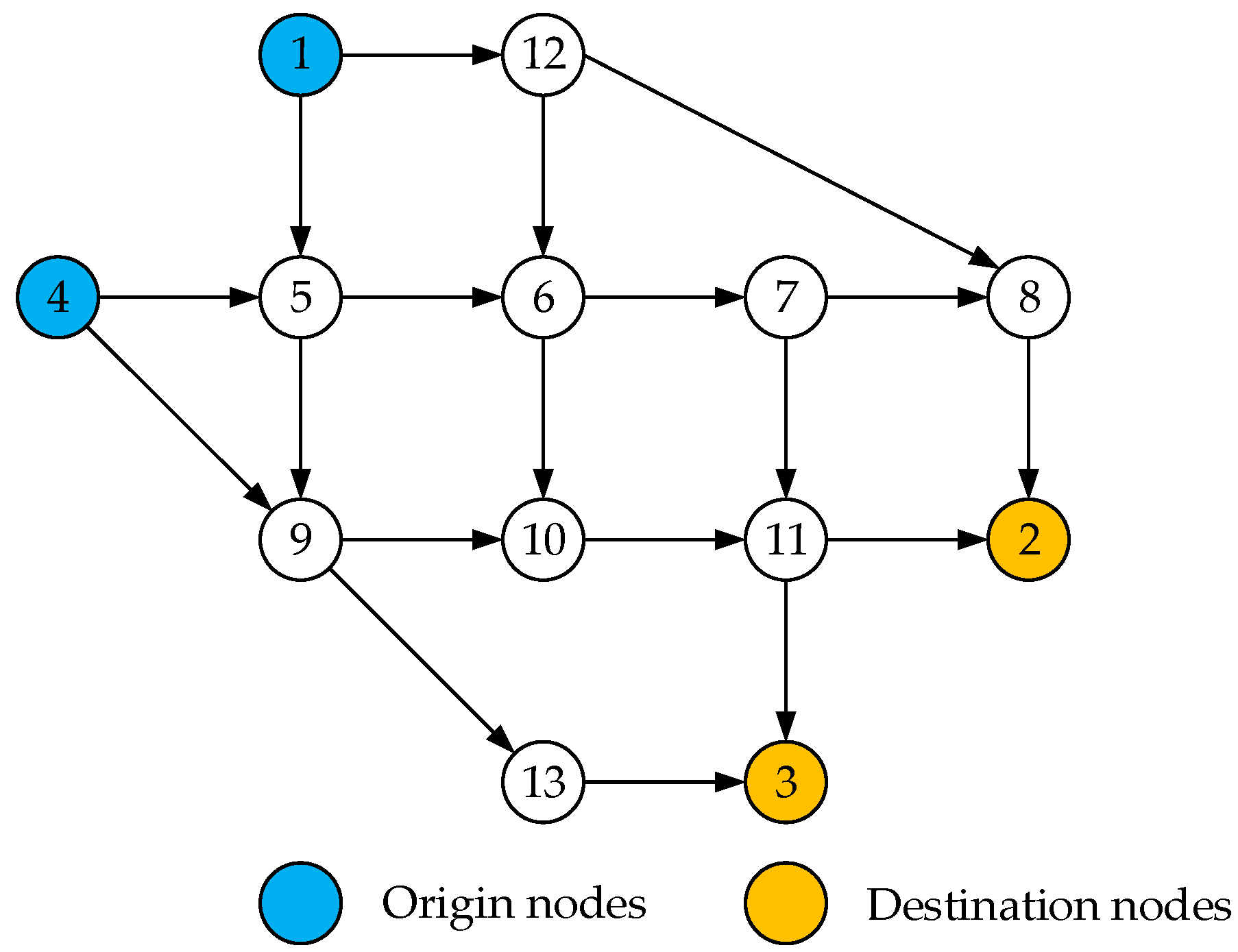
In this section, we present numerical examples to demonstrate the proposed models. In order to validate the proposed model and algorithm, first we solve the model [ARMSTLP-CN] in the Nguyen-Dupius network shown in Figure 1 [2]. This small network consists of 13 nodes, 19 links, and four O–D pairs. Free-flow travel time, capacity, and electricity consumption of each link are tabulated in

Table 2. Nguyen-Dupius network characteristics.

Link	Capacity (veh/h)	Distance (mile)	Travel Time (min)
1-5	40	14.7	9.8
1-12	30	18.9	12.6
4-5	30	18.9	12.6
4-9	30	25.2	16.8
5-6	50	6.3	4.2
5-9	30	18.9	12.6
6-7	50	10.5	7.0
6-10	40	27.3	18.2
7-8	50	10.5	7.0
7-11	40	18.9	12.6
8-2	40	18.9	12.6
9-10	30	21	14.0
9-13	30	18.9	12.6
10-11	30	12.6	8.4
11-2	30	18.9	12.6
11-3	30	16.8	11.2
12-6	30	14.7	9.8
12-8	30	29.4	19.6
13-3	30	23.1	15.4

.

Moreover, we have some assumptions. The total budget $B$ is 38. The initial state of charge electricity $L_0$ for all O–D pairs is 20 $\mathrm{kWh}$, while the battery capacity $L_{max}$ is 24 $\mathrm{kWh}$, $m^a$ which means the comfortable electricity range for agent $a$ is set to 2 $\mathrm{kWh}$. $\overline{w}$ is equal to 0.29$\mathrm{kWh}/\mathrm{mi}$, which expresses the energy consumption rate of BEVs. The maximum and minimum number of chargers, $z_{max}^{\phi }$ and $z_{min}^{\phi }$, are set to 5 and 2 respectively.

Table 3. O–D demand.

O/D	2	3
1	20	30
4	30	20

suggests the different O–D pairs demand.

Table 4. O–D energy recharged.

O–D Pair	The Number of Agents Recharged (kWh)	The Amount of Energy Recharged (kWh)
1-2	10	14.88
1-3	30	69.00
2-4	30	62.91
3-4	20	29.76
Total	90	176.55

can show that the number of agents recharged and the amount of energy recharged of different O–D pairs. In addition, parameters of different chargers such as $c{f}_{\phi }^f$, $c{f}_{\phi }^v$ and ${\epsilon }^{\phi }$ are showed at

Table 5. Parameter setting of different chargers.

$\mathit{\phi }$	$\mathit{c}{\mathit{f}}_{\mathit{\phi }}^{\mathit{f}}$	$\mathit{c}{\mathit{f}}_{\mathit{\phi }}^{\mathit{v}}$	${\mathit{\epsilon }}^{\mathit{\phi }}(\mathbf{min}/\mathbf{kWh})$
1	1	0.8	41.67
2	1.5	5	10
3	2.5	10	0.67

. The location and types of the charging station are given in

Table 6. Charging station construction program.

Node	The Type of Chargers	Chargers Number	The Number of Agents Recharged
5	2	2	20
8	1	3	10
9	3	2	10

.

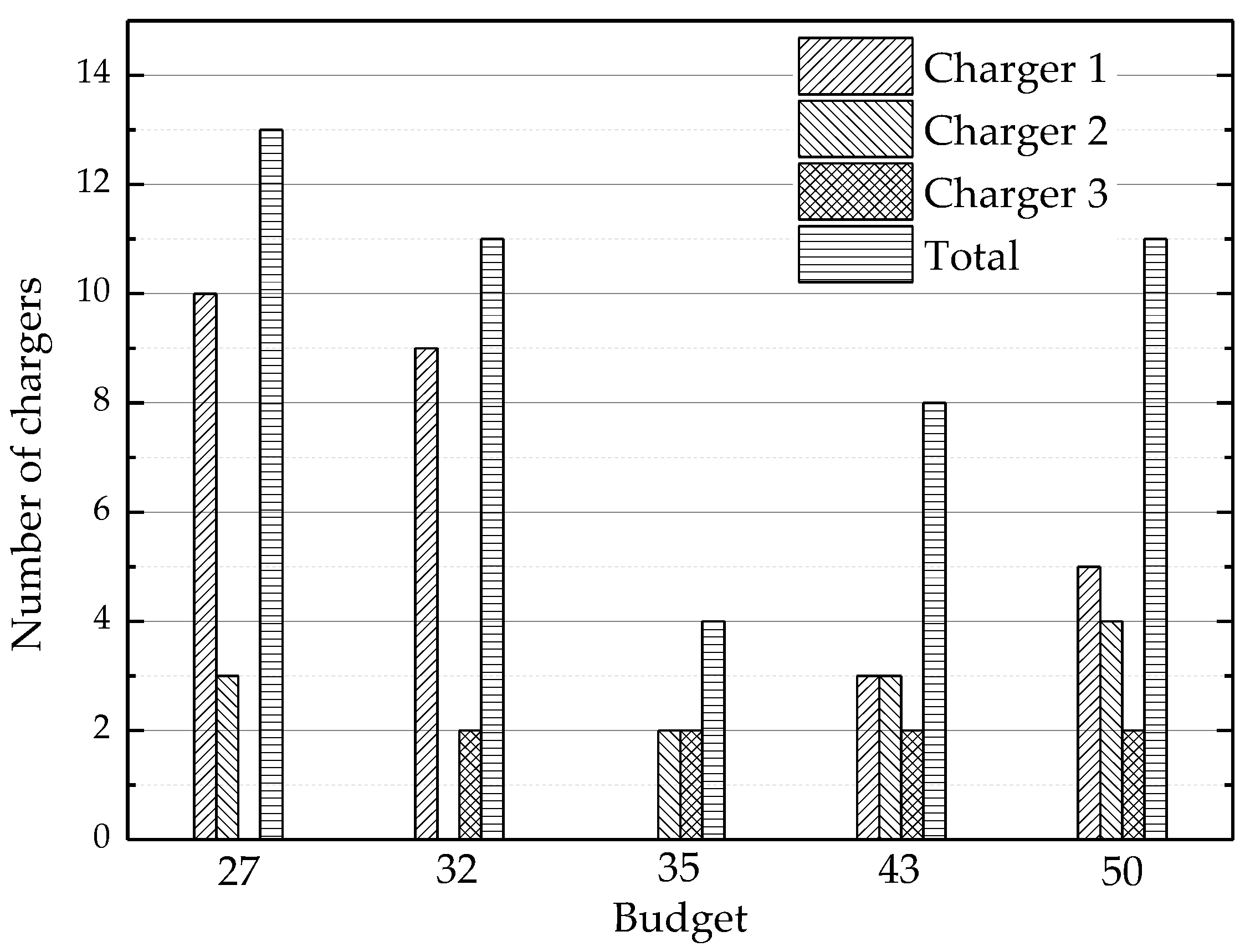
4.2. Considering Different Total Budget

We know that different sizes and different types of charging station have a great influence on the equilibrium. Moreover, the total budget determines the sizes and types of the charging station. So in the next, we consider about the different total budget, and any other parameters are the same. The different total budget considered are 27, 32, 35, 43, and 50. The initial state of charge is set to 20$\mathrm{kWh}$ and the range anxieties of all agents are set to 2$\mathrm{kWh}$. The result considering different total budget is shown in the figures below.

From Figure 2, we can see that with the budget is increasing, the total trip time is a decreasing trend. This phenomenon is easy to understand. When the budget is increasing, more charging stations can be built, and also we can choose the charger with faster charging rates to shorten the charging time. This inference is confirmed in Figure 3. From Figure 3, we can see that when the budget is low, more chargers of type 1 are built, and the number of chargers of types 2 and 3 is relatively small. As the total budget is increasing, more chargers of types 2 and 3 are built. When we see the total number of chargers, we may find that the trend is to decrease first and then increase. Maybe we can infer that there is an optimal value between the budget values we set. We can also know the number and distribution of charger station under different budget levels in

Table 7. The number and distribution of charger station under different budget levels.

Node	Total Budget
	27	32	35	43	50
1	0	0	0	0	0
2	0	0	0	0	0
3	0	0	0	0	0
4	0	0	0	0	0
5	5	0	0	0	4
6	0	0	2	3	0
7	0	4	0	0	0
8	0	5	0	0	0
9	3	2	2	2	2
10	0	0	0	0	0
11	0	0	0	0	0
12	5	0	0	3	5
13	0	0	0	0	0

. The difference of budget value setting will result in different distribution locations and sizes of charging stations.

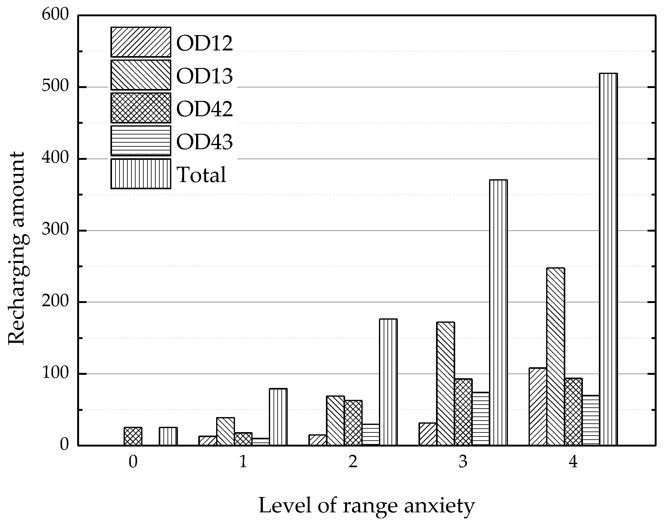
4.3. Considering Different Levels of Range Anxiety

Due to the uncertainty of the fuel economy, drivers of BEVs may not feel comfortable fully depleting their batteries. Instead, they likely reserve a safety margin to hedge against variations of energy consumption, and they would not allow the remaining battery range to fall below it.

Before this study, some scholars have studied the problem of range anxiety [1,2]. As we all know, when the range anxiety is larger, the limited driving ranges is smaller, so more charging stations should be built. Therefore, in this section, we consider the impact of different levels of range anxiety on the size and type of charging stations. The five different levels of range anxiety considered are 0, 1, 2, 3, and 4, which is shown in

Table 8. The number and distribution of chargers under different levels of range anxiety.

Node	Range Anxiety
	0	1	2	3	4
1	0	0	0	0	0
2	0	0	0	0	0
3	0	0	0	0	0
4	0	0	0	0	0
5	0	0	2	0	0
6	0	0	0	3	2
7	0	0	0	0	0
8	0	5	3	2	0
9	0	0	2	2	2
10	3	0	0	0	0
11	0	5	0	0	0
12	0	0	0	0	0
13	0	5	0	0	2

. The results are as follows.

Figure 4 shows the amount of recharge for different levels of range anxiety. It is obvious that when range anxiety equals zero, agents of O–D pair 12, O–D pair 13, and O–D pair 43 do not need to recharge, only O–D pair 42 has to recharge. Moreover, as the range anxiety increases, the amount of recharge of each O–D pair increases significantly. This phenomenon can be explained that when range anxiety become greater, the number and the amount of recharge will increase to ensure a remaining battery state of charge of no less than the comfortable range. The cost of different range anxieties can be shown from Figure 5. In the same way, as the amount of recharging increases, the cost to build charging stations will rise and the total trip time will increase. We also can find the type and quantity distribution of chargers changed under different levels of range anxiety in Figure 6.

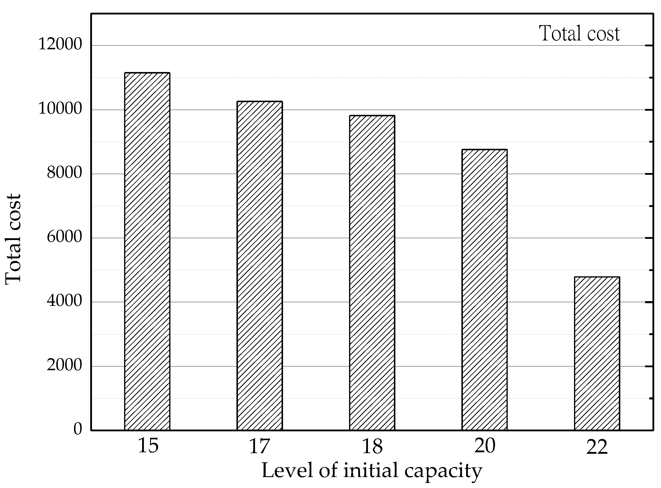
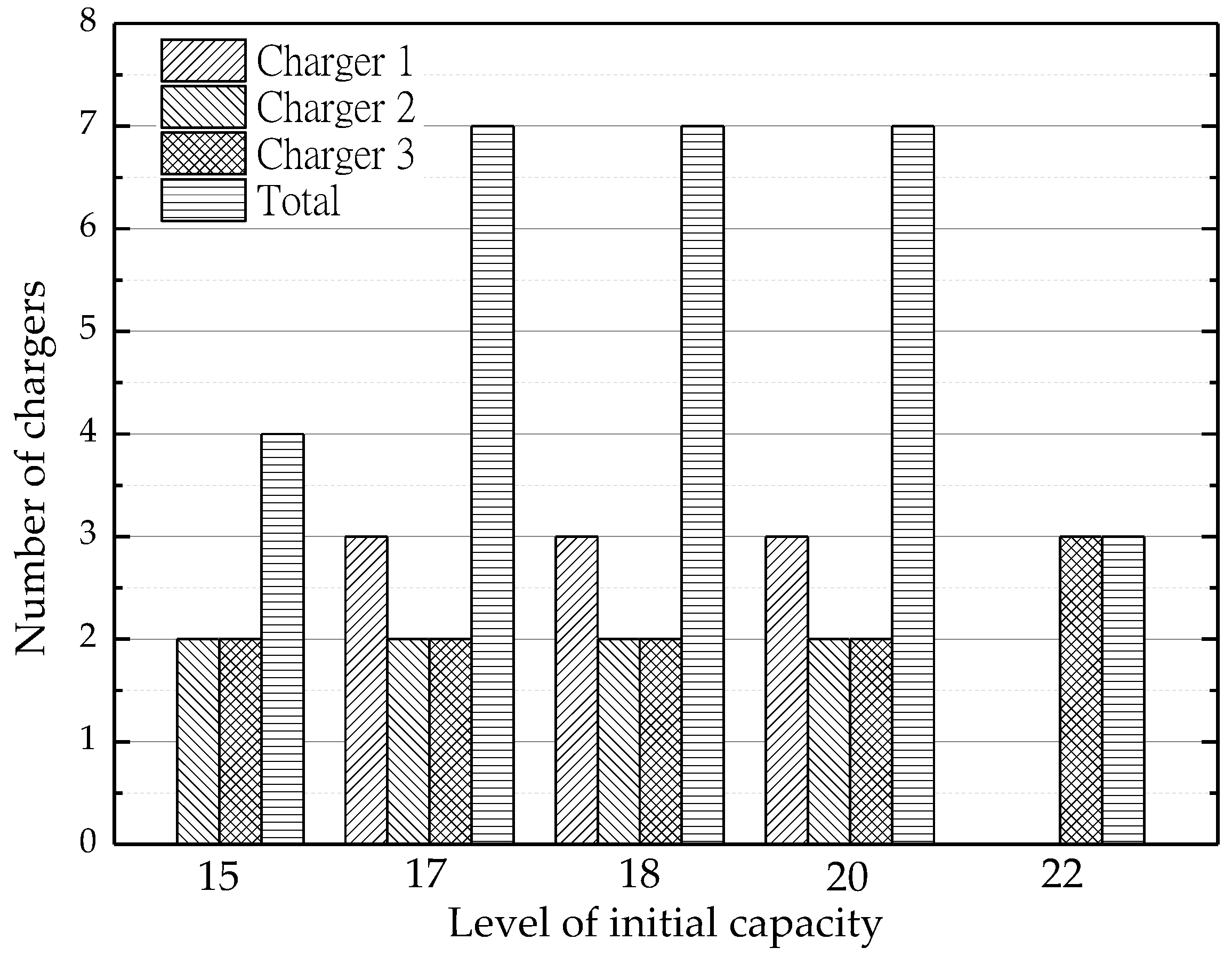
4.4. Considering Different Levels of Initial Capacity

The different initial charge has a great influence on the user’s charging behavior. In this essay we set the initial capacity to be 15, 17, 18, 20, and 22$\mathrm{kWh}$, respectively, in order to see the change of the cost, the amount of recharge, and the distribution of charger. The amount of recharge for different levels of initial capacity can be seen in Figure 7. Figure 8 shows the cost of different levels of initial capacity, and Figure 9 indicates that the type and quantity distribution of chargers under different levels of initial capacity.

In this article, we set the battery capacity to 24$\mathrm{kWh}$. From Figure 7, we can see that the when the initial charge is low, the amount of recharge is at a high level. As the initial charge is increasing, the amount of recharge of each O–D pair is decreasing. And when the initial capacity is set at 22 $\mathrm{kWh}$, only O–D42 needs to recharge. It is obvious in Figure 8 that the larger the initial capacity set, the smaller the cost is. This is a result of that when the initial capacity is higher, a little amount of recharge need to be provided, so the total cost will be reduced. From Figure 9 we can infer that the effect of initial charge on the distribution of different charging piles is not great. When the initial charge is set to be 17, 18, and 20 $\mathrm{kWh}$, we see the distribution is not changed. As for

Table 9. The number and distribution of chargers under different levels of initial capacity.

Node	Initial Capacity (kWh)
	15	17	18	20	22
1	0	0	0	0	0
2	0	0	0	0	0
3	0	0	0	0	0
4	0	0	0	0	0
5	0	3	0	2	0
6	2	0	0	0	0
7	0	2	2	0	0
8	0	0	0	3	0
9	2	2	2	2	3
10	0	0	3	0	0
11	0	0	0	0	0
12	0	0	0	0	0
13	0	0	0	0	0

, although the number and type of chargers have not changed, the distribution of charging stations has changed clearly.

4.5. A Lager Example

In order to verify the correctness and rationality of the model effectively, the larger Sioux Falls network shown in Figure 10 is presented as an example. This network consists of 24 nodes, 76 links, and 576 O–D pairs. The free-flow travel time, capacity, and distance of each link are reported in

Table 10. Sioux Falls network characteristics.

Link	Capacity (veh/h)	Distance (mile)	Travel time (min)	Link	Capacity (veh/h)	Distance (mile)	Travel Time (min)
1-2	30	5.4	3.6	13-24	45	3.6	2.4
1-3	60	3.6	2.4	14-11	20	3.6	2.4
2-1	20	5.4	3.6	14-15	20	4.5	3
2-6	40	4.5	3	14-23	25	3.6	2.4
3-1	20	3.6	2.4	15-10	25	5.4	3.6
3-4	20	3.6	2.4	15-14	20	4.5	3
3-12	55	3.6	2.4	15-19	20	3.6	2.4
4-3	25	3.6	2.4	15-22	20	3.6	2.4
4-5	35	1.8	1.2	16-8	20	4.5	3
4-11	25	5.4	3.6	16-10	30	4.5	3
5-4	25	1.8	1.2	16-17	20	1.8	1.2
5-6	20	3.6	2.4	16-18	20	2.7	1.8
5-9	20	4.5	3	17-10	25	6.3	4.2
6-2	25	4.5	3	17-16	25	1.8	1.2
6-5	25	3.6	2.4	17-19	30	1.8	1.2
6-8	40	1.8	1.2	18-7	20	1.8	1.2
7-8	30	2.7	1.8	18-16	30	2.7	1.8
7-18	25	1.8	1.2	18-20	20	3.6	2.4
8-6	25	1.8	1.2	19-15	20	3.6	2.4
8-7	30	2.7	1.8	19-17	20	1.8	1.2
8-9	25	3	2	19-20	30	3.6	2.4
8-16	20	4.5	3	20-18	20	3.6	2.4
9-5	20	4.5	3	20-19	20	3.6	2.4
9-8	30	3	2	20-21	25	5.4	3.6
9-10	25	2.7	1.8	20-22	20	4.5	3
10-9	30	2.7	1.8	21-20	25	5.4	3.6
10-11	20	4.5	3	21-22	20	1.8	1.2
10-15	20	5.4	3.6	21-24	30	2.7	1.8
10-16	25	4.5	3	22-15	20	3.6	2.4
10-17	20	6.3	4.2	22-20	20	4.5	3
11-4	20	5.4	3.6	22-21	25	1.8	1.2
11-10	20	4.5	3	22-23	20	3.6	2.4
11-12	30	5.4	3.6	23-14	30	3.6	2.4
11-14	30	3.6	2.4	23-22	20	3.6	2.4
12-3	30	3.6	2.4	23-24	30	1.8	1.2
12-11	20	5.4	3.6	24-13	20	3.6	2.4
12-13	60	2.7	1.8	24-21	30	2.7	1.8
13-12	35	2.7	1.8	24-23	25	1.8	1.2

. In this article, we choose eight O–D pairs to make it easier. The O–D demands are listed in

Table 11. O–D demand.

O/D	13	24	21	20
1	10	12	10	15
2	10	15	10	10

. As for parameter settings, such as total budget $\mathrm{B}$ and battery capacity $L_{max}$, the comfortable electricity range for agent $a$, $m^a$, and so on. are the same as Section 4.1. The only different parameter is the initial state of charge electricity $L_0$, which is set to be 4$\mathrm{kWh}$. Parameter settings of different chargers is listed in

Table 12. Parameter settings of different chargers.

$\mathit{\phi }$	$\mathit{c}{\mathit{f}}_{\mathit{\phi }}^{\mathit{f}}$	$\mathit{c}{\mathit{f}}_{\mathit{\phi }}^{\mathit{v}}$	${\mathit{\epsilon }}^{\mathit{\phi }}(\mathbf{min}/\mathbf{kWh})$
1	1	0.5	41.67
2	1.5	4	10
3	2.5	8	0.67

.

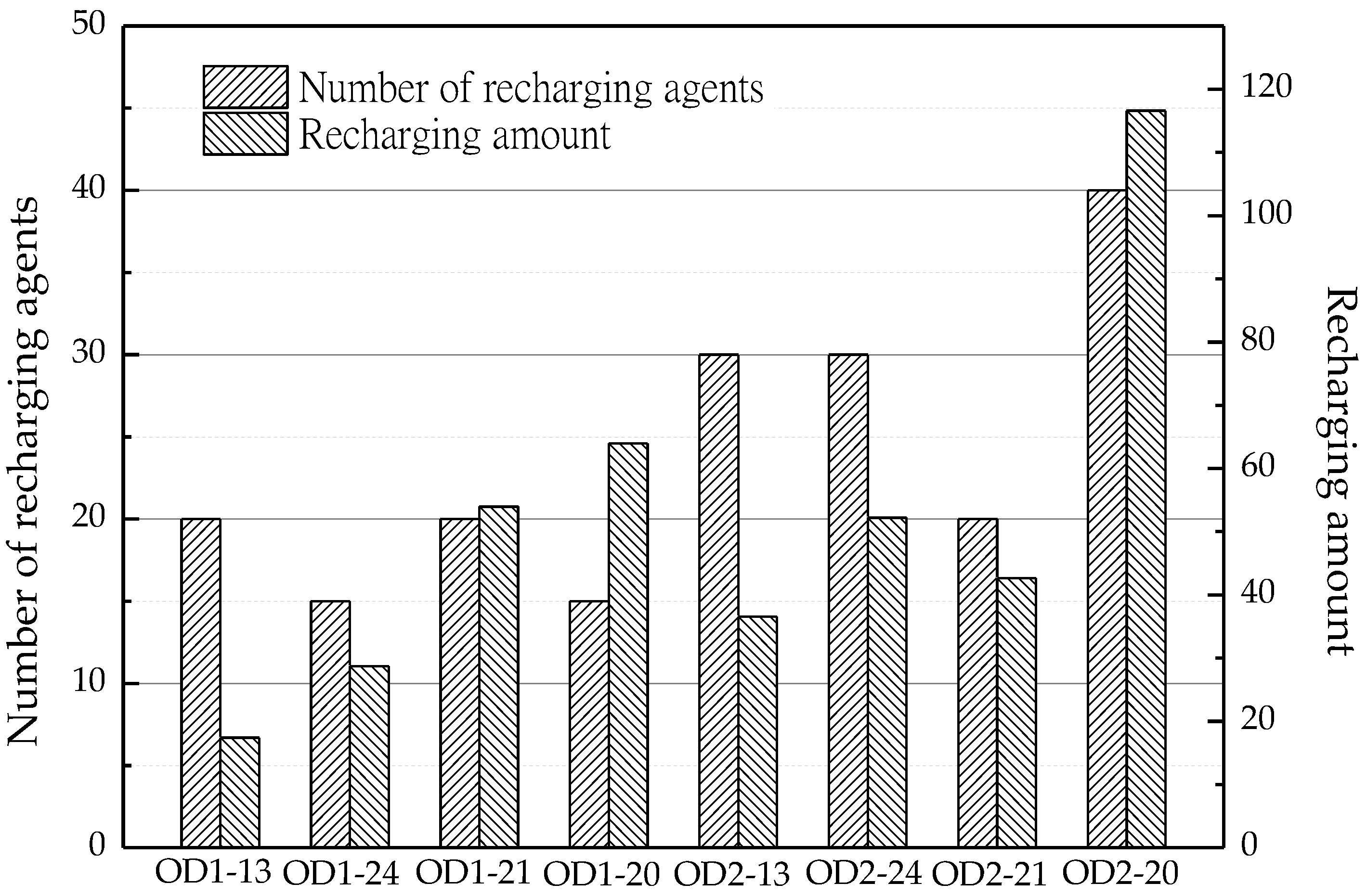
GAMS is used to solve the problem. From the results, we can get that the total travel time is 5571.586 when the parameter is set to the mentioned situation above. Other results are shown in the table below.

Table 13. O–D energy recharged.

O–D pair	The Number of Agents Recharged	The Amount of Energy Recharged (kWh)
1-13	20	17.420
1-24	15	28.725
1-21	20	53.960
1-20	15	63.960
2-13	30	36.550
2-24	30	52.215
2-21	20	42.640
2-20	40	116.600
Total	190	412.070

shows that when the network reach equilibrium, the number of agents recharged and the amount of energy recharged in each O–D pair. We can see the number of agents recharged in pair 1-20 is the largest, which has 40 agents recharged in this O–D pair and the amount of energy recharged is 116.600 kWh. This phenomenon can be inferred from the Sioux Falls network. In the network node 2 is relatively far away from node 20, so agents in this O–D pair may need more electricity. This is more intuitive in Figure 11. The location and types of the different charging station are given in

Table 14. Charging station construction program.

Node	The Type of Chargers	Chargers Number	The Number of Agents Recharged		The Amount of Energy Recharged
			Number	Percentage (%)	Number	Percentage (%)
1	1	5	60	32	36.60	9
3	3	4	130	68	375.47	91

. We can see that the number of agents recharged in charger 1 accounts for 32 percent of the total, but the amount of energy only accounts for 9 percent. We may infer that a large number of people in a charging station does not mean a large amount of charging. In addition, we can see that one charging station is built in the original node, which is also reasonable because when the electric vehicle starts to drive with the low initial capacity, it might recharge in the original node.

5. Conclusions and Future Research

In this paper, the location distribution of different size and types of charging stations is considered. By considering the different types of charging stations, different charging demands of different users can be satisfied. The difference in the size of the charging stations reduces the overall government budget for the construction of the stations, while meeting the minimum travel time for travelers. This paper also considers the user’s anxious mileage and other factors comprehensively, making our problem more practical. In addition, we verify the validity of the model through two networks. In the Nguyen-Dupius network, we observe the final charging station location and the size and type of charging station by changing the total budget of the establishment of charging station, the initial electric quantity, and the anxious range of agents. The final result is practical, indicating that the model is reasonable and feasible. To make the result more convincing, we applied the model to the Sioux Falls network which has more nodes, more sections, and is more complex. In conclusion, the results show that our study is meaningful and practical.

Finally, the objective of our study is only BEVs, which are relatively simple compared to those mixed BEV and gasoline vehicles. We need to consider both requirements in a hybrid network. However, the methods mentioned in our paper can be used for reference in future studies. Especially regarding the size and type of charging station, it is of great reference significance for future consideration of the location of battery exchange station or wireless charging station. Last but not least, the dynamic model considering travel time and actual travel distance is more realistic than the static model in this paper.

Furthermore, several ways can be extended in this model. An effective solution algorithm should be designed in the future. In the real world, the scale of the network is much higher than the network proposed in the paper, so the solution rate of the commercial solver may be greatly limited, and we cannot find the optimal solution within a certain calculation time. Therefore, more efficient algorithms can be expected in future work. Furthermore, the maximum travel distance can vary according to environmental factors, including weather, temperature, and so on. These factors will exist in reality and will greatly affect the operation of the vehicle, especially electric vehicles. Therefore, these various factors should be reflected in future studies.