Dynamic Connectedness of International Crude Oil Prices: The Diebold–Yilmaz Approach

College of Economics and Management, Huazhong Agricultural University, Wuhan 430070, China
*
Author to whom correspondence should be addressed.
Sustainability 2018, 10(9), 3298; https://doi.org/10.3390/su10093298
Submission received: 18 July 2018
/
Revised: 3 September 2018
/
Accepted: 12 September 2018
/
Published: 14 September 2018
(This article belongs to the Section Energy Sustainability)
Abstract
:Connectedness is the key to modern risk measurement and management. This study investigates the international connectedness of crude oil prices and explores its time-varying characteristics based on a connectedness measurement framework using daily international crude oil prices. The international connectedness of crude oil prices is investigated from three perspectives: total connectedness, total directional connectedness, and pairwise directional connectedness. We find that the total connectedness of crude oil prices is 67.3%. We also find that the crude oil prices of Tapes, Daqing, Dubai and Minas are highly affected by Brent and WTI (West Texas Intermediate) crude oil prices. Furthermore, WTI and Brent are the price makers of international crude oil prices, while Tapes, Daqing, Dubai and Minas are price takers. From the perspective of pairwise directional connectedness, we find that the degree of pairwise directional connectedness between Brent and WTI are high. Finally, the structure of international crude oil markets stays the same even after market shocks. The main contributions of this study are identification of dynamic connectedness and presentation of the network connectedness of international crude oil prices.
1. Introduction
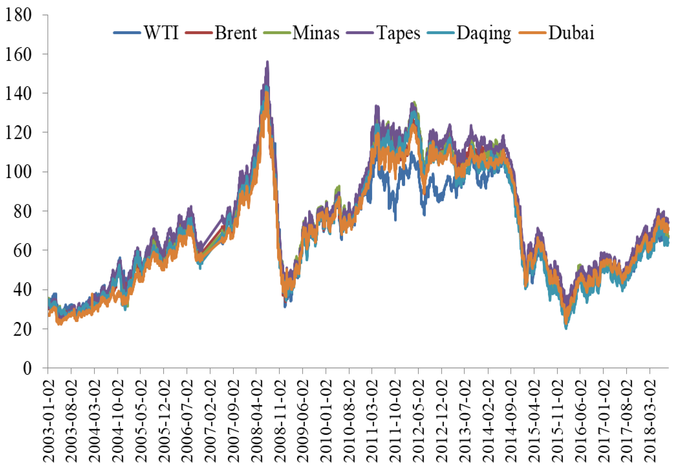
Over the years, international crude oil prices have experienced sharp rises and falls and have attracted extensive attention from policymakers, researchers, and investors [1]. As shown in Figure 1, for example, the crude oil price of WTI (West Texas Intermediate) was $65 per barrel in May 2007, rising to $145.3 per barrel around July 2008, and falling to $31.3 per barrel on 22 December 2008. Another significant characteristic of the international oil market is that the crude oil prices of WTI, Brent, Minas, Tapes, Daqing, and Dubai have synchronous trends. We can see in Figure 1 that the plots of these six international crude oil prices nearly always overlap. Although the crude oil price of WTI differed from the other five crude oil prices during 2011–2014, the fluctuation trends remained generally the same. For example, six of the international crude oil prices were at the bottom in August 2011, June 2012 and March 2013, while they peaked in February 2012, August 2012 and September 2013. This co-movement of international crude oil prices has also been of great interest to policymakers, researchers, and investors.
Is the international crude oil market “a great pool”? There are two opposing views on this issue: one holds that the international crude oil market is fragmented, and is therefore not a great pool. One of the key proponents of this view is Weiner, who analyzes patterns of price adjustment and considers that the world oil market is far from completely unified. The correlation and regression results of price adjustment across regions indicates a surprisingly high degree of regionalization. Weiner insists that there are many importing-country governments that seek special arrangements for a “secure supply” from exporters and many oil exporters have also sought “secure outlets” for their crude oil [3]. These arrangements make no sense if the world crude oil market is integrated. In contrast, the other side of the argument is that the international crude oil market is integrated, namely, that the international crude oil market is “a great pool”. A representative of the “great pool” view is Adelman, who argues that the world oil market behaves as “one great pool” where changes in market conditions in one area quickly affect other geographic areas [4,5]. He clarifies that the crude oil market is unified based on the “Law of One Price”. According to this notion, arbitrage opportunities will realign prices if crude oil prices diverge by amounts greater than the differences implied by transportation costs and quality. With the economic globalization process, an increasing number of scholars agree that the international crude oil market is unified in the manner of a “great pool” [6,7,8,9].
In this study, we attempt to deepen the “great pool” question, using international crude oil prices. We start our study by raising a few questions: What is the total connectedness of international crude oil prices? What are the time-varying characteristics of the connectedness? How can the connectedness of international crude oil prices be presented in a more intuitive way? Existing studies have not discussed these issues thoroughly. An in-depth analysis of these questions will help forecast the trends of international crude oil prices, reduce losses caused by the great volatility of crude oil prices, and promote sustainable development.
Answering these questions requires a multidimensional directional study of the connectedness of international crude oil prices. By connectedness, we mean the state of being linked, being related, or being connected. Existing studies have proposed several methods for measuring relevance. We divide these studies into two categories. One category discusses the relevance of different variables. Representative methods include cointegration test and Granger causality test [10,11], correlation coefficients [12,13], Baba, Engle, Kraft and Kroner-generalized autoregressive conditional heteroscedastic (BEKK–GARCH) models [14,15], principal-components analysis [16], and others. Another category focuses on the measurement of risk spillovers and the contribution of individual institutions to systemic risk. Representative methods include marginal expected shortfall (MES) [17] and the conditional value at risk (CoVaR) [18,19]. Both categories are based on market data and have their own advantages. However, these categories have the following two shortcomings. The first is the lack of a unified framework that considers the relevance of different dimensions; for example, correlation-based methods are limited to the correlation between variables, without considering the relevance of the entire system. The second shortcoming is that most of these methods can only show correlation levels, ignoring the directions of connectedness. In fact, the directions of connectedness of international crude oil prices are as important as its levels for risk measurement and control of crude oil markets. To address these problems, Diebold and Yilmaz developed and applied a unified framework for conceptualizing and empirically measuring connectedness at various levels, from pairwise through system-wide [20]. Based on assessing shares of forecast error variation in different crude oil prices due to shocks arising elsewhere, this method not only measures the levels of connectedness but also identifies the directions of connectedness [21]. In addition, the method is closely linked to the network structure diagram, which can visualize the levels and directions of connectedness [22,23].
To accurately measure the connectedness of international crude oil prices, this study draws on the connectedness measurement framework proposed by Diebold and Yilmaz [20]. This approach measures connectedness from three perspectives: total connectedness, total directional connectedness, and pairwise directional connectedness. Total connectedness is an overall description of the degree of system connectedness. Total directional connectedness from others represents the share of volatility shocks received from others in the total forecast error variance of each price, while total directional connectedness to others stands for each price’s contribution to the others’ forecast error variances. Pairwise directional connectedness indicates the directional connectedness between two variables. We first perform a full-sample analysis to explore static connectedness, and then turn to a rolling-sample to explore dynamic connectedness. We use the daily data of six international crude oil prices over the sample period from 2 January 2003 to 17 August 2018. The main contribution of this study is the identification of dynamic connectedness through rolling sample windows and visualizing the network connectedness of international crude oil prices using network structure diagrams.
2. Materials and Method
2.1. Data Description
Considering data availability and sample representativeness, we select the crude oil prices of the WTI, Brent, Dubai, Daqing, Minas and Tapes as the sample. Crude oil prices of WTI, Brent and Dubai are three important international oil price benchmarks. China is the world’s second largest crude oil consumer, and the crude oil price of Daqing is the most representative oil price for China. The crude oil price of Minas in Indonesia is the benchmark price for most of the intermediate, low-sulphur crude oil in Asia, while the crude oil price of Tapes in Malaysia is a typical price for Southeast Asia. Therefore, the crude oil prices of WTI, Brent, Dubai, Daqing, Minas and Tapes that we select are highly representative. High-frequency data are more useful in reflecting actual prices and reducing measurement errors. We use high-frequency daily data over the sample period of 2 January 2003 to 17 August 2018, resulting in 3351 samples for each price. All these data are from the Wind database, and the unit of crude oil prices is USD per barrel. Table 1 shows the data’s descriptive statistics. The augmented Dickey–Fuller (ADF) tests show that the series of crude oil prices in the major international markets are non-stationary, while the series in first differences are stationary.
2.2. Connectedness Measurement Approach
Diebold and Yilmaz propose a method for measuring connectedness based on assessing the decomposition of forecast error variance [20]. This is intimately related to the familiar econometric notion of a variance decomposition, in which the forecast error variance of variable i is decomposed into parts attributed to the various variables in the system. The connectedness measurement approach is a measuring tool and has little to do with statistical tests. For a multivariate time series, we can first fit a vector autoregressive model, then establish an H period-ahead forecast, and finally decompose the forecast error variance for each variable with respect to shocks from the same or other variables at time t. We use to denote the ij-th H-step forecast error variance. In other words, represents the fraction of variable i’s H-step forecast error variance due to shocks in variable j. It is worth noting that . The key is , which emphasizes that our connectedness measures are based on the “non-own” or “cross”.
Consider an N-dimensional covariance-stationary data-generating process with orthogonal shocks: , , . Note that need not be diagonal. Contemporaneous aspects are summarized in and dynamic aspects in . The transformation of via variance decompositions is needed to reveal and compactly summarize connectedness. Diebold and Yilmaz propose a connectedness table [20] (see Table 2), which proves central for understanding the various connected measures and their relationships. The main upper-left N × N block, which is called a “variance decomposition matrix”, denoted by , contains the variance decompositions. The connectedness table increase the with a bottom row containing column sums, a rightmost column containing row sums, and a bottom-right element containing the grand average.
The connectedness measures are based on the “non-own” or “cross”, which means that we focus on the off-diagonal entries of the variance decomposition matrix . These off-diagonal entries are the parts of the N forecast error variance decomposition of relevance and they represent pairwise directional connectedness in particular. We define the pairwise directional connectedness from j to i as follows:
Since in general , there are separate pairwise directional connectedness measures. Then we define the net pairwise directional connectedness as
Now consider the off-diagonal row or column sums of . The off-diagonal row sums, labelled “from others” in the connectedness table, give the share of H-step forecast-error variance of variable coming from shocks arising in all other variables (not one single other variable). The off-diagonal column sums, labelled “to others”, provide the share of the H-step forecast-error variance of variable going to shocks arising in all other variables. We define total directional connectedness from others to i as
and total directional connectedness to others from j as
There are 2N total directional connectedness measures. Just as for net pairwise directional connectedness, we define net total directional connectedness of variable i as
There are N net total directional connectedness measures. Finally, the sum of “from” columns or “to” rows measures total connectedness, which is the grand total of the off-diagonal entries in . We define total connectedness as
There is just one total connectedness measure, which distills a system into a single number.
For the case of orthogonal shocks discussed so far, the variance decompositions are easily calculated, because the variance of a weighted sum is a weighted sum of variance. However, in the case of non-orthogonal shocks, the variance decompositions are not as easily calculated as before, because, in the non-orthogonal case, traditional methods such as Cholesky-factor identification may be sensitive to ordering. Following Diebold and Yilmaz [20], a generalized Vector Autoregression (VAR) decomposition that is invariant to ordering, proposed by Koop et al. and Pesaran and Shin [24,25], is used. The H-step generalized variance decomposition (GVD) matrix with entries, which is
where is a selection vector with j-th element unity and zeros elsewhere, is the coefficient matrix in the infinite moving average representation of the non-orthogonalized VAR, is the covariance matrix of the shock vector, and is its j-th diagonal element. Because we work in the Koop–Pesaran–Potter–Shin generalized VAR framework and shocks are not necessarily orthogonal in this framework, sums of forecast error variance contributions are not necessarily unity. Hence, we normalize each entry of the generalized variance decomposition (GVD) matrix by the row sum to obtain pairwise directional connectedness from j to i:
By construction, and . We can calculate the generalized connectedness measures using .
3. Results and Discussion
3.1. Connectedness Analysis Using the Full Sample
Table 3 shows the connectedness of major international crude oil prices using the full sample. Many features are notable: the diagonal elements (own connectedness) appear to be the largest individual elements of the table, but total directional connectedness (from others or to others) tends to be much larger, and total connectedness is close to 70%. Next, we analyze Table 3 in the order of total connectedness, total directional connectedness, and pairwise directional connectedness.
3.1.1. Total Connectedness Using the Full Sample
Total connectedness is an overall description of the degree of system connectedness. As shown in the bottom right corner of Table 3, total connectedness is 67.3%, which indicates that about 70% of the change in international crude oil prices is caused by the mutual influence of the major international crude oil prices. This result is supported by a series of studies [5,6,7,8,9], which confirm that the world crude oil market is as a “great pool”, and the elements that constitute the world oil markets have been closely linked.
3.1.2. Total Directional Connectedness Using the Full Sample
The values in the rightmost column of Table 3 are the total directional connectedness from other prices to each of the six prices and represent the share of volatility shocks received from other prices in the total variance of the forecast error for each price. By definition, it is equal to 100% minus the own share of the total forecast error variance. As seen from Table 3, the total directional connectedness in the “From” column ranges between 46.7% and 75.8%. There are four prices more than 70%, including Tapes (75.8%), Daqing (75.5%), Dubai (73.7%) and Minas (71.5%), which indicates that these four crude oil prices are highly affected by other prices. WTI (46.7%) and Brent (60.7%) are less affected by other crude oil prices.
Similarly, the values in the second row from the bottom of Table 3 represent the total directional connectedness from each price to other prices and stand for each price’s contribution to the others’ forecast error variances. The results from Table 3 show that the total directional connectedness in the “To” column has large differences, varying from 54.4% (Minas) to 81.0% (WTI). According to the characteristics of the values, we know that crude oil prices of Brent (80.1%) and WTI (81.0%) have greater impact on other prices.
The bottommost row provides the net total directional connectedness, which indicates the difference between total directional connectedness to others and total directional connectedness from others (to–from). The net total directional connectedness of WTI and Brent is positive at 34.3% and 19.5%, respectively, illustrating that the impact from these two crude oil prices to other prices is greater than that from other prices. In other words, these two prices play a dominant role in the international crude oil market, so they are price makers. In contrast, Minas (−17.0%), Tapes (−10.9%), Daqing (−9.5%) and Dubai (−16.3%) have negative values in net total directional connectedness; that is, they are price takers in the international crude oil market. Existing studies support this view: Wlazlowski et al. pointed out that WTI and Brent are the price makers of international crude oil prices, while Daqing, Minas and Tapes crude oil markets are price takers [26].
3.1.3. Pairwise Directional Connectedness Using the Full Sample
The off-diagonal elements of the 6 × 6 matrix in Table 3 indicate the directional connectedness between two prices. For example, the value 20.3 in row 3, column 2, represents the percent of forecast error variance of Brent crude oil price due to shocks from WTI. From the perspective of pairwise directional connectedness, we have the following findings.
First, the pairwise directional connectedness between Brent and WTI appears to be very high. The highest observed pairwise directional connectedness is from Brent to WTI (25.1%), followed by that from WTI to Brent (20.3%). WTI and Brent crude are the most influential benchmarks for light crude oil in North America and Europe, respectively [27]. In the decades before 2010, the prices of WTI and Brent moved in tandem [27]. Maslyuk and Smyth highlighted a co-integration of WTI and Brent prices in spot as well as in futures markets [28]. Two things may contribute to this result. On the one hand, a large amount of crude oil trade may regulate supply and demand situations. Crude oil trade follows the “Law of One Price”, and crude oil prices in various regions gradually converge due to space arbitrage by crude oil traders. On the other hand, there is information spillover in the futures market [29,30]. There are two major crude oil futures exchanges: the New York Mercantile Exchange (NYMEX) and the London International Petroleum Exchange (IPE). The crude oil futures market is dominated by these two competing benchmark grades. As benchmarks, WTI and Brent provide a reference price against which oil around the world is traded at a premium or discount [31]. Information about crude oil is transmitted among crude oil exchanges; thus, these two crude prices are closely linked.
Second, for China’s Daqing crude oil price, Minas and Tapes have greater impacts. The pairwise directional connectedness from Minas and Tapes to Daqing are 16.6% and 15.9%, which are higher than for other prices. On the contrary, for Minas and Tapes, Daqing has greater impact than other crude oil prices. The pairwise directional connectedness from Daqing to Minas and Tapes are 18.2% and 16.5%, respectively. This may be because the spatial distance of Daqing, Tapes and Minas is relatively short, and the Tapes and the Minas crude oil spot prices are employed as the related time series based on China’s oil pricing rules [32].
3.2. Connectedness Analysis Under Rolling Sample
Connectedness analysis using the full sample focuses on the static connectedness of crude oil prices, so it does not help us understand the dynamics of connectedness [33]. The following subsections discuss connectedness under rolling sample. Unlike using the full sample, rolling sample analysis can reveal the dynamic connectedness of crude oil prices. Drawing on Diebold and Yilmaz’s method [20], this study sets the rolling sample period as 200 days and the forecast period as 12 days. We analyze the dynamic connectedness in the order of total connectedness, total directional connectedness, and pairwise directional connectedness.
3.2.1. Total Connectedness Under Rolling Sample
As seen from Figure 2, the total connectedness of crude oil prices in the six international markets hovered between 47.6% and 77.1% from 27 October 2003 to 17 August 2018. During the sample period, four distinct fluctuation peaks are revealed.
The first peak occurred from May 2008 to February 2009. The total connectedness of crude oil prices among the six markets rose rapidly from 69.5% to the peak of 76.6%, and then plummeted to 72.7%. During the same period, international crude oil prices experienced an unusual period of increasing and dropping suddenly and sharply. For example, the crude oil price of WTI was 65 USD per barrel in May 2007, rising to $145.3 per barrel around July 2008 and then falling to $31.3 per barrel on 22 December 2008. The Brent, Minas, Tapes, Daqing and Dubai crude oil prices showed similar trends. The simultaneous soaring and slumping of international oil prices during this period may have been affected by the subprime crisis. Existing studies suggest that the subprime crisis lowered the level/trend and increased the volatility of crude oil prices [34,35]. With the spread of the subprime crisis, market elements in global oil markets linked tightly, increasing the connectedness among various crude oil prices.
The second peak appeared during the period from August 2009 to June 2010. The total connectedness of the six international crude oil prices rose from 70.5% to 76.5%, and then declined to 71.7%. Although the financial crisis led to shrinking oil demand, the effect gradually disappeared with the Organization of the Petroleum Exporting Countries (OPEC) member countries’ implementation of a production reduction agreement. Coupled with the devaluation of the US dollar and the renewed involvement of international speculative capital, the international oil price rose to around $ 80 per barrel and maintained this status for one year. The influences of exchange rates and speculation on crude oil price were extensively confirmed [36,37]. The tightening of supply and the influence of financial factors led to a similar trend in various international crude oil prices, resulting in a significant fluctuation in total connectedness from August 2009 to June 2010.
During the period from June 2012 to September 2014, the third peak of total connectedness occurred. The total connectedness of the six crude oil prices rose from 64.6% in June 2012 to 72.0% in May 2013, and then fell to 69.0% in September 2014. International crude oil prices remained stable at the high level of $90–$120 per barrel during this period. There are some possible factors that contributed to this phenomenon. First, the quantitative easing monetary policy implemented by the Federal Reserve during the period lowered the US dollar exchange rate [38], which pushed up the international crude oil price. Second, in mid-2012, the United States and the European Union imposed sanctions on Iran due to Iran’s nuclear activities [39]. The lowering of the US dollar exchange rate and the Iranian oil embargo have had an important impact on the global crude oil market, causing various international crude oil prices to remain at a high level during this period, and connectedness of the international crude oil prices was once again very high.
The last obvious peak of total connectedness occurred from September 2014 to the end of 2017. The total connectedness of the six crude oil prices rose from 59.0% in September 2014 to 76.7% in March 2016 and remained stable at over 75% for a long time, falling to 70.9% at the end of 2017. Overall, international crude oil prices in 2016–2017 were on the rise in the range of $20–$70 per barrel. The rise in oil prices and increase in the connectedness of international crude oil prices during this period were driven by multiple factors, such as the attack on the Nigerian oil infrastructure [40], the Kuwaiti oil workers’ strike, and the OPEC members’ agreement to reach a production cut [41].
3.2.2. Total Directional Connectedness Under Rolling Sample
Figure 3, Figure 4 and Figure 5 show the total directional connectedness of the six international crude oil prices. Figure 3 shows the total directional connectedness to others, Figure 4 shows the total directional connectedness from others, and Figure 5 shows the net total directional connectedness.
Compared with the plots of total directional connectedness to others, the plots of total directional connectedness from others are much smoother. That is, the former fluctuates frequently and strongly, while the latter fluctuates less frequently with lower amplitude. This may be because the total directional connectedness from others is less than 100%, but the total directional connectedness to others may be more than 100% [20].
The variation of net total directional connectedness over the rolling sample windows resembles the variation in the total directional connectedness to others [20]. According to the definition, the net total directional connectedness is the difference between total directional connectedness to others and total directional connectedness from others. Because the plots of total directional connectedness from others are much smoother than the plots of total directional connectedness to others, the trends of net total directional connectedness are similar to those of total directional connectedness to others.
3.2.3. Pairwise Directional Connectedness Under Rolling Sample
Analyzing the pairwise directional connectedness under rolling sample can help us identify the dynamics of pairwise directional connectedness among international crude oil prices. In particular, by comparing the pairwise directional connectedness before and after the events, we can deepen our understanding of how the connectedness measures across international crude oil prices vary over time. Because we set the rolling sample period as 200 days and the forecast period as 12 days, we ended up with 6748 pairwise directional measures and 3374 net pairwise directional measures. It is impossible to present all the plots in the confines of this paper. Instead, to make the analysis more typical, we present and discuss the net pairwise directional connectedness during the most critical stage. Therefore, we use July 2008 as a base period to compare and analyze the net pairwise directional connectedness before and after this severely turbulent period. Based on this, we choose the net pairwise directional connectedness of international crude oil prices on 2 May 2008 and 30 October 2008 for comparative analysis. For a more intuitive observation, we use network structure diagrams to show the net pairwise directional connectedness between crude oil prices [22,42]. As shown in Figure 6, the nodes represent the prices. The larger size and the deeper color of the nodes mean that the impacts of this price on other prices are greater. The lines between nodes represent the degree of connectedness. The deeper the color of the lines, the higher the degree of connectedness. The arrows in the lines represent the direction of the connectedness. We use the Gephi software to draw the network structure diagrams.
Figure 6 illustrates how the total connectedness of the six international crude oil prices rose rapidly from 73.4% on 2 May to 76.9% on 30 October. As shown in Figure 6, we believe that the pattern of the net pairwise directional connectedness of international crude oil prices did not change significantly after international crude oil prices surged and plummeted. We can easily judge from (a) and (b) of Figure 6 that WTI and Brent play a leading role in the connectedness. On 2 May, the net pairwise directional connectedness from WTI to Brent, Dubai, Minas, Daqing and Tapes are the top five among all of that day’s net pairwise directional connectedness. On 30 October, the net pairwise directional connectedness from WTI to Tapes, Minas, and Daqing are the top three among all of that day’s net pairwise directional connectedness. The node color of WTI and Brent are deeper and their node sizes are larger. This result further confirms the previous view that WTI and Brent are the price makers of international crude oil prices, while Dubai, Daqing, Minas and Tapes are price takers.
3.3. Robustness Test
To verify the robustness of our results to the choice of the forecast horizon and rolling sample window, we consider forecast horizons of 6 days, 12 days and 18 days, and rolling sample windows of 100 days, 200 days and 300 days. Next, we observe whether changes in the forecast horizons and the rolling sample windows cause significant variations in total connectedness. Figure 7 shows the results. On the one hand, we fix the forecast horizons and observe the impact of the window widths. In the case of a forecast horizon of 6 days, as the window width increases, the total connectedness decreases slightly, but the trend and volatility of total connectedness do not change. This rule is also true in the rolling sample windows of 12 days and 18 days. On the other hand, the rolling sample window is fixed to observe the impact of the forecast horizons. Under the condition that the rolling window is 100 days, as the forecast horizon increases, total connectedness increases slightly, but the trend and volatility of total connectedness do not change. This rule also applies to the cases of 200 days and 300 days. In short, changes in the forecast horizon and rolling sample window have a minor impact on the relative value of total connectedness, but will not affect the trends or volatility of total connectedness. Therefore, the conclusion of this study is robust to the choice of forecast horizons and rolling sample window widths.
4. Conclusions
Observing that major international crude oil prices have similar trends, we raise the question of whether or not the international crude oil market is “a great pool”. There has been a great deal of debate in the literature on this question. This study attempts to deepen this question using price data within a unified framework. Based on the framework of connectedness measurement proposed by Diebold and Yilmaz, we investigate the network connectedness of international crude oil prices and explore its time-varying characteristics, using daily data of six international crude oil prices over the period from 2 January 2003 to 17 August 2018.
From the perspective of total connectedness, we find that the total connectedness of the six international crude oil prices is 67.3%, with four distinct fluctuations during the sample period. From the perspective of total directional connectedness, the crude oil prices of Tapes, Daqing, Dubai and Minas are highly affected by other crude prices, and crude oil prices of Brent and WTI have a greater impact on other crude oil prices. Furthermore, according to the results of net total directional connectedness, WTI and Brent are the price makers of international crude oil price, while Dubai, Daqing, Minas and Tapes are price takers. From the perspective of pairwise directional connectedness, the degrees of pairwise directional connectedness between Brent and WTI are high. Finally, we find that the structure of international crude oil markets stays the same even after market shocks.
The main contribution of this study is the identification of the dynamic and network connectedness of international crude oil prices. First, we set the rolling sample period as 200 days and the forecast period as 12 days to explore the time-varying characteristics of total connectedness, total directional connectedness, and pairwise directional connectedness. This is beneficial for us to understand the nature of connectedness. Second, for a more intuitive observation, we draw network structure diagrams to show the net pairwise directional connectedness between prices. Comparing the net pairwise directional connectedness in network structure diagrams before and after the events, we can deepen our understanding of connectedness of international crude oil prices.
In addition, we believe that these findings are relevant for policymakers and investors. We show that the international connectedness of crude oil prices is strong and clarify the time-varying characteristics. For policymakers, considering the connectedness of international crude oil prices and its time-varying characteristics is conducive to predicting the effectiveness of energy policies. The effectiveness of government policies depends to a large extent on whether the impact of the policy action extends to other regions or remains confined to the local market [3]. For investors, considering the network connectedness of international crude oil prices and its time-varying characteristics is helpful for judging the trends and relationships of different crude oil prices, which will help to identify more arbitrage opportunities and avoid investment failures in both spot and futures markets.
There are some shortcomings in our study. First, this study focuses on the connectedness measurements of international crude oil prices and its time-varying characteristics, ignoring the economic mechanism of connectedness, which needs to be explored in the future. Second, six major crude oil prices are just a part of international crude oil prices. High frequency data are more likely to reflect the relationship among variables; however, high frequency data are rare. Due to the scarcity of daily data, we are only able to capture the six major international crude oil prices of WTI, Daqing, Dubai, Brent, Minas and Tapes. Fortunately, these six international crude oil prices are common and important in world oil markets, and thus, they may be considered representative of the world crude oil markets.
Author Contributions
Conceptualization: X.X.; Data curation: J.H.; Formal analysis: X.X.; Methodology: X.X.; Writing—original draft: J.H.; Writing—review & editing, X.X.
Funding
National Natural Science Foundation of China: 71703049. Humanities and Social Science Project of the Ministry of Education of China: 17YJC790173. Fundamental Research Funds for the Central Universities: 2662016QD053.
Acknowledgments
This research was funded by the National Natural Science Foundation of China (No. 71703049), the Humanities and Social Science Project of the Ministry of Education of China (No. 17YJC790173) and the Fundamental Research Funds for the Central Universities (No. 2662016QD053).
Conflicts of Interest
The authors declare no conflict of interest.
References
- Lundgren, A.I.; Milicevic, A.; Uddin, G.S.; Kang, S.H. Connectedness network and dependence structure mechanism in green investments. Energy Econ. 2018, 72, 145–153. [Google Scholar] [CrossRef]
- Wind. Available online: http://www.wind.com.cn (accessed on 10 May 2018).
- Weiner, R.J. Is the World Oil Market “One Great Pool”? Energy J. 1991, 12, 95–107. [Google Scholar] [CrossRef]
- Adelman, M.A. International Oil Agreements. Energy J. 1984, 5, 1–9. [Google Scholar] [CrossRef]
- Adelman, M.A. “Is the World Oil Market One Great Pool?”—Comment. Energy J. 1992, 13, 157–158. [Google Scholar] [CrossRef]
- Bachmeier, L.J.; Griffin, J.M. Testing for Market Integration Crude Oil, Coal, and Natural Gas. Energy J. 2006, 27, 55–71. [Google Scholar] [CrossRef]
- Bentzen, J. Does OPEC influence crude oil prices? Testing for co-movements and causality between regional crude oil prices. Appl. Econ. 2007, 39, 1375–1385. [Google Scholar] [CrossRef]
- Fattouh, B. The dynamics of crude oil price differentials. Energy Econ. 2010, 32, 334–342. [Google Scholar] [CrossRef]
- Dai, Y.-H.; Xie, W.-J.; Jiang, Z.-Q.; Jiang, G.J.; Zhou, W.-X. Correlation structure and principal components in the global crude oil market. Empir. Econ. 2016, 51, 1501–1519. [Google Scholar] [CrossRef] [Green Version]
- Ziramba, E. Price and income elasticities of crude oil import demand in South Africa: A cointegration analysis. Energy Policy 2010, 38, 7844–7849. [Google Scholar] [CrossRef]
- Uri, N.D. Changing crude oil price effects on US agricultural employment. Energy Econ. 1996, 18, 185–202. [Google Scholar] [CrossRef]
- Huang, X.; Zhou, H.; Zhu, H. A framework for assessing the systemic risk of major financial institutions. J. Bank. Financ. 2009, 33, 2036–2049. [Google Scholar] [CrossRef]
- Patro, D.K.; Qi, M.; Sun, X. A simple indicator of systemic risk. J. Financ. Stab. 2013, 9, 105–116. [Google Scholar] [CrossRef]
- Bekiros, S.D.; Diks, C.G.H. The relationship between crude oil spot and futures prices: Cointegration, linear and nonlinear causality. Energy Econ. 2008, 30, 2673–2685. [Google Scholar] [CrossRef] [Green Version]
- Power, G.J.; Vedenov, D.V.; Anderson, D.P.; Klose, S. Market volatility and the dynamic hedging of multi-commodity price risk. Appl. Econ. 2013, 45, 3891–3903. [Google Scholar] [CrossRef]
- Billio, M.; Getmansky, M.; Lo, A.W.; Pelizzon, L. Econometric measures of connectedness and systemic risk in the finance and insurance sectors. J. Financ. Econ. 2012, 104, 535–559. [Google Scholar] [CrossRef] [Green Version]
- Acharya, V.V.; Brownlees, C.; Engle, R.; Farazmand, F.; Richardson, M.; Cooley, T.F.; Walter, I. Measuring Systemic Risk; New York University Stern School of Business: New York, NY, USA, 2010; pp. 85–119. [Google Scholar]
- Acharya, V.; Engle, R.; Richardson, M. Capital Shortfall: A New Approach to Ranking and Regulating Systemic Risks. Am. Econ. Rev. 2012, 102, 59–64. [Google Scholar] [CrossRef]
- Adrian, T.; Brunnermeier, M. CoVaR. FRB of New York Staff Report No. 348. 2011. Available online: https://ssrn.com/abstract=1269446 (accessed on 15 June 2018).
- Diebold, F.X.; Yılmaz, K. On the network topology of variance decompositions: Measuring the connectedness of financial firms. J. Econom. 2014, 182, 119–134. [Google Scholar] [CrossRef] [Green Version]
- Maghyereh, A.I.; Awartani, B.; Bouri, E. The directional volatility connectedness between crude oil and equity markets: New evidence from implied volatility indexes. Energy Econ. 2016, 57, 78–93. [Google Scholar] [CrossRef] [Green Version]
- Demirer, M.; Diebold, F.X.; Liu, L.; Yilmaz, K. Estimating global bank network connectedness. J. Appl. Econom. 2017, 33, 1–15. [Google Scholar] [CrossRef] [Green Version]
- Diebold, F.X.; Yilmaz, K. Trans-Atlantic Equity Volatility Connectedness: U.S. and European Financial Institutions, 2004–2014. J. Financ. Econom. 2016, 14, 81–127. [Google Scholar] [CrossRef]
- Koop, G.; Pesaran, M.H.; Potter, S.M. Impulse response analysis in nonlinear multivariate models. J. Econom. 1996, 74, 119–147. [Google Scholar] [CrossRef]
- Pesaran, H.H.; Shin, Y. Generalized impulse response analysis in linear multivariate models. Econ. Lett. 1997, 58, 17–29. [Google Scholar] [CrossRef]
- Wlazlowski, S.; Hagströmer, B.; Giulietti, M. Causality in crude oil prices. Appl. Econ. 2011, 43, 3337–3347. [Google Scholar] [CrossRef] [Green Version]
- Chen, W.; Huang, Z.; Yi, Y. Is there a structural change in the persistence of WTI–Brent oil price spreads in the post-2010 period? Econ. Model. 2015, 50, 64–71. [Google Scholar] [CrossRef]
- Maslyuk, S.; Smyth, R. Cointegration between oil spot and future prices of the same and different grades in the presence of structural change. Energy Policy 2009, 37, 1687–1693. [Google Scholar] [CrossRef]
- Han, L.; Xu, Y.; Yin, L. Does investor attention matter? The attention-return relationships in FX markets. Econ. Model. 2018, 68, 644–660. [Google Scholar] [CrossRef]
- Wu, Y.; Han, L.; Yin, L. Our currency, your attention: Contagion spillovers of investor attention on currency returns. Econ. Model 2018, in press. [Google Scholar] [CrossRef]
- Scheitrum, D.P.; Carter, C.A.; Revoredo-Giha, C. WTI and Brent Futures Pricing Structure. Energy Econ. 2018, 72, 462–469. [Google Scholar] [CrossRef]
- Jia, X.; An, H.; Fang, W.; Sun, X.; Huang, X. How do correlations of crude oil prices co-move? A grey correlation-based wavelet perspective. Energy Econ. 2015, 49, 588–598. [Google Scholar] [CrossRef]
- Fernández-Rodríguez, F.; Gómez-Puig, M.; Sosvilla-Rivero, S. Using connectedness analysis to assess financial stress transmission in EMU sovereign bond market volatility. J. Int. Financ. Mark. Inst. Money 2016, 43, 126–145. [Google Scholar] [CrossRef]
- Yang, W.; Han, A.; Hong, Y.; Wang, S. Analysis of crisis impact on crude oil prices: A new approach with interval time series modelling. Quant. Financ. 2016, 16, 1–12. [Google Scholar] [CrossRef]
- Yoshino, N.; Hesary, F.T. Monetary policy and oil price fluctuations following the subprime mortgage crisis. Inter. J. Monetary Econ. Financ. 2014, 7, 157–174. [Google Scholar] [CrossRef]
- Kim, J.M.; Jung, H. Relationship between oil price and exchange rate by FDA and copula. Appl. Econ. 2018, 50, 2486–2499. [Google Scholar] [CrossRef]
- Juvenal, L.; Petrella, I. Speculation in the Oil Market. J. Appl. Econ. 2015, 30, 621–649. [Google Scholar] [CrossRef]
- Ogawa, E.; Wang, Z. Effects of Quantitative Easing Monetary Policy Exit Strategy on East Asian Currencies. Dev. Econ. 2016, 54, 103–129. [Google Scholar] [CrossRef]
- Farzanegan, M.R.; Parvari, M.R. Iranian-Oil-Free Zone and international oil prices. Energy Econ. 2014, 45, 364–372. [Google Scholar] [CrossRef] [Green Version]
- Yeeles, A.; Akporiaye, A. Risk and resilience in the Nigerian oil sector: The economic effects of pipeline sabotage and theft. Energy Policy 2016, 88, 187–196. [Google Scholar] [CrossRef]
- Ratti, R.A.; Vespignani, J.L. OPEC and non-OPEC oil production and the global economy. Energy Econ. 2015, 50, 364–378. [Google Scholar] [CrossRef]
- Han, L.; Wu, Y.; Yin, L. Investor attention and currency performance: International evidence. Appl. Econ. 2017, 50, 2525–2551. [Google Scholar] [CrossRef]
Figure 1.
Crude oil prices in USD per barrel (raw data). Source: Wind [2].
Figure 1.
Crude oil prices in USD per barrel (raw data). Source: Wind [2].

Figure 2.
Total connectedness of international crude oil prices under rolling sample. Source: Own calculation.
Figure 2.
Total connectedness of international crude oil prices under rolling sample. Source: Own calculation.

Figure 3.
Total directional connectedness to others: (a) From crude oil price of WTI, Brent and Minas; (b) From crude oil price of Tapes, Daqing and Dubai. Source: Own calculation.
Figure 3.
Total directional connectedness to others: (a) From crude oil price of WTI, Brent and Minas; (b) From crude oil price of Tapes, Daqing and Dubai. Source: Own calculation.

Figure 4.
Total directional connectedness from others: (a) To crude oil price of WTI, Brent and Minas; (b) To crude oil price of Tapes, Daqing and Dubai. Source: Own calculation.
Figure 4.
Total directional connectedness from others: (a) To crude oil price of WTI, Brent and Minas; (b) To crude oil price of Tapes, Daqing and Dubai. Source: Own calculation.

Figure 5.
Net total directional connectedness: (a) Of crude oil price of WTI, Brent and Minas; (b) Of crude oil price of Tapes, Daqing and Dubai. Source: Own calculation.
Figure 5.
Net total directional connectedness: (a) Of crude oil price of WTI, Brent and Minas; (b) Of crude oil price of Tapes, Daqing and Dubai. Source: Own calculation.

Figure 6.
Net pairwise directional connectedness: (a) Before July 2008; (b) After July 2008. Note: TC stands for Total Connectedness. Source: Own calculation.
Figure 6.
Net pairwise directional connectedness: (a) Before July 2008; (b) After July 2008. Note: TC stands for Total Connectedness. Source: Own calculation.

Figure 7.
Robustness test of total connectedness: (a) H=6 days; (b) H=12 days; (c) H=18 days. Source: Own calculation.
Figure 7.
Robustness test of total connectedness: (a) H=6 days; (b) H=12 days; (c) H=18 days. Source: Own calculation.


Table 1.
Descriptive statistics of crude oil prices in major international markets.
| WTI | Brent | Minas | Tapes | Daqing | Dubai | |
|---|---|---|---|---|---|---|
| Mean | 69.6 | 73.1 | 73.5 | 76.9 | 70.6 | 70.3 |
| Median | 68.3 | 69.2 | 68.8 | 73.1 | 65.8 | 66.6 |
| Max | 145.3 | 144.2 | 149.7 | 156.1 | 143.4 | 140.5 |
| Min | 23.7 | 22.8 | 22.3 | 25.5 | 20.1 | 22.4 |
| Std Dev | 24.9 | 29.1 | 30. 6 | 30.5 | 29.6 | 28.7 |
| Skewness | 0.2 | 0.2 | 0.3 | 0.2 | 0.3 | 0.2 |
| Kurtosis | 2.1 | 1.8 | 1.8 | 1.9 | 1.8 | 1.8 |
| ADF | −2.2 | −1.8 | −1.8 | −1.8 | −1.7 | −1.8 |
| 1st-ADF | −60.3 *** | −56.3 *** | −39.9 *** | −61.1 *** | −58.9 *** | −60.5 *** |
Note: *** indicate significance at 1%.
Table 2.
Schematic of a connectedness table.
| From Others | |||||
|---|---|---|---|---|---|
| To others |
Table 3.
Connectedness table of international crude oil price using the full sample.
| WTI | Brent | Minas | Tapes | Daqing | Dubai | From | |
|---|---|---|---|---|---|---|---|
| WTI | 53.3 | 25.1 | 4.5 | 6.4 | 5.4 | 5.3 | 46.7 |
| Brent | 20.3 | 39.3 | 8.5 | 11.5 | 10.2 | 10.1 | 60.7 |
| Minas | 12.6 | 12.1 | 28.5 | 15.3 | 18.2 | 13.2 | 71.5 |
| Tapes | 17.0 | 15.0 | 13.2 | 24.2 | 16.5 | 14.0 | 75.8 |
| Daqing | 14.6 | 13.7 | 15.9 | 16.6 | 24.5 | 14.7 | 75.5 |
| Dubai | 16.5 | 14.2 | 12.3 | 15.1 | 15.7 | 26.3 | 73.7 |
| To | 81.0 | 80.1 | 54.4 | 64.9 | 66.0 | 57.4 | 67.3 |
| NET | 34.3 | 19.5 | −17.0 | −10.9 | −9.5 | −16.3 |
© 2018 by the authors. Licensee MDPI, Basel, Switzerland. This article is an open access article distributed under the terms and conditions of the Creative Commons Attribution (CC BY) license (http://creativecommons.org/licenses/by/4.0/).
Share and Cite
MDPI and ACS Style
Xiao, X.; Huang, J. Dynamic Connectedness of International Crude Oil Prices: The Diebold–Yilmaz Approach. Sustainability 2018, 10, 3298. https://doi.org/10.3390/su10093298
AMA Style
Xiao X, Huang J. Dynamic Connectedness of International Crude Oil Prices: The Diebold–Yilmaz Approach. Sustainability. 2018; 10(9):3298. https://doi.org/10.3390/su10093298
Chicago/Turabian StyleXiao, Xiaoyong, and Jing Huang. 2018. "Dynamic Connectedness of International Crude Oil Prices: The Diebold–Yilmaz Approach" Sustainability 10, no. 9: 3298. https://doi.org/10.3390/su10093298
Note that from the first issue of 2016, this journal uses article numbers instead of page numbers. See further details here.