Abstract
In the summer of 2011, a change in the Kansas laws came into effect, increasing the speed limit on a selected set of freeway sections from 70 mph to 75 mph. Higher speeds were thought to have economic benefits, mostly because the travel time reduction means people reach their destinations more quickly. In this study, the sections where the speed limits remained unchanged, are compared to freeway sections that have been influenced by speed limit increase, to evaluate safety effectiveness. The study utilizes the before-and-after study with comparison group method to assess the safety effects provided in the Highway Safety Manual (HSM). Two crash datasets, obtained by considering three years before and three years after the speed limit increase, were compared in order to evaluate the safety effects of the speed limit change. The crash modification factors (CMFs) were estimated, which showed that there was a 27% increase in total crashes and a 35% increase in fatal and injury crashes across all sections after the speed limit change, and these increases were statistically significant at 95% confidence level. These confounding results show that the speed limit increase has not been beneficial for traffic safety in Kansas, and hence it is important to be cautious in such future situations. Also, additional data have been presented which would be beneficial in identifying and understanding any behavior change in drivers following a speed limit increase.
1. Introduction
The link between the speed limit and the number of crashes is a topic of interest to vehicle insurance firms and the general public. Transportation agencies have a very important role in identifying proper speed limits for all public roadways within their jurisdiction. Speed limits are an important tool for drivers to be notified about the allowable speed for driving on a specific roadway. According to Bill HB 2192, the secretary of transportation in Kansas was allowed to change the speed limit from 70 mph to 75 mph on about 800 miles of interstates, in July 2011. Some criteria that were identified as important attributes when determining the appropriate speed limit value for the selected sites were the roadways classification as rural or urban, the number of vehicles passing on the road, traffic volumes, and geometric characteristics [1]. Geometric characteristics of a road layout include, shoulder type, the degree of curves, median type, median width, number of lanes, lane width, rumble strip type, and cross slope.
A report released by the U.S. National Transportation Safety Board (NTSB) examined the reasons for speeding-related passenger vehicle crashes. The NTSB found that 16.66% out of 26% of total fatal crashes on freeways are related to speeding in Kansas in the year 2014 (Figure 1). This means that speeding has become a significant contributing factor in fatal crashes, specifically on freeways compared to other types of roadways in recent years for the state of Kansas [2]. Similarly, increasing the speed limit could influence the crash severity and may result in a higher number of fatal crashes. Accordingly, the purpose of this study was to assess the safety consequences of the roadways related to the speed limit increase. The three different before-and-after studies identified by the Highway Safety Manual [3] are: Observational before/after evaluation studies (simple before/after study), observational before/after evaluation studies using the Safety Performance Functions (SPFs)—the Empirical Bayes (EB) method, and observational before/after evaluation study using the comparison group method. The before-and-after study with comparison group method was utilized in this study to determine the impact of speed limit change on the number of crashes on freeways. This method also considers information about non-treated sections, on which the speed limit did not change, making it a more reasonable methodology to evaluate safety effectiveness.
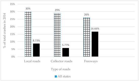
Figure 1.
Speeding related fatal crashes in all states versus Kansas in 2014.
Previous research has evaluated the impact of speed limit changes on traffic safety and commonly presented thought-provoking results about safety effects. The safety effects of speed limit reduction were considered from 55 mph to 45 mph on a number of highways in Belgium. Odds ratio were estimated for injury crashes and the results showed a decrease on injury crashes after speed limit decrease [4]. A before-and-after study using Empirical Bayes method, for 6 years before and 6 years after a speed limit reduction from 80 km/h to 60 km/h was used on some multi-lane divided highways, which resulted in a 7.5% crash reduction in Oslo, Norway [5]. A study by Renski and Khattak, evaluated the impact of multiple speed limit increases on interstate highways in North Carolina, and estimated that the crash modification factors (CMFs) according to the before-and-after study approach revealed an increase in the probability of injuries and fatalities on treated sites where speed limits were increased [6]. The speed limit increase from 55 mph to 65 mph was considered on rural interstates and limited access highways in Illinois [7]. Based on the auto-regressive integrated moving average models (ARIMA) method for time series data, a higher speed limit was found to have resulted in an increase in deaths and injuries per month for rural areas [7]. According to current literature, speed limit increases may not always exacerbate the crash experience. Speed limit increases, from 55 mph to 65 mph on most urban interstates and rural two-lane highways, were considered in Kansas along with a speed limit increase from 55 mph to 70 mph on rural multi-lane highways [8]. Researchers applied a before-and-after study with a comparison group method and revealed that there was no statistically significant increase in fatal crashes on rural and urban interstate highways; however, there was a statistically significant increase in fatal crashes on two-lane rural highways. Rural interstates are usually more influenced by crash severity increase compared with urban interstates, since there are no residential areas and drivers are more likely to drive at speeds above the legal limit in rural areas where the enforcement levels are low. For example, a study by Ledolter, Johannes, and Chan examined a speed limit increase from 55 mph to 65 mph on Iowa rural interstates, and according to their before-and-after analysis, the number of statewide fatal crashes increased by 20% as a result of the speed limit change [9].
2. Data
The treated group includes all road sections that experienced an increase in the speed limit from 70 mph to 75 mph. The non-treated group also includes a similar set of road sections where the speed limit did not change and remained at 70 mph during the entire time period. The treated and non-treated groups were identified with assistance from Kansas Department of Transportation (KDOT). The geometric characteristics for non-treated sections, such as shoulder type, the degree of curves, median type, median width, the number of lanes, lane width, rumble strip type, and cross slope were similar to those of treated sections. The geometric characteristic similarity helped to conduct the before-and-after study by considering these variables for both treated and non-treated sections in order to evaluate the speed limit change during the after-period. Other data related to each section such as the annual average daily traffic (AADT), the length of each section, fatal, injury, and property damage only (PDO) crashes were collected from the Kansas Crash Analysis and Recording System (KCARS) database for both groups during a three-year period before and after the speed limit change [10]. The year 2011 was not considered because the speed limit change occurred that year.
The non-treated group contained 4-lane divided segments with a speed limit of 70 mph and the treated group contained 4-lane divided segments with a speed limit of 75 mph, allowing their comparison. The average length and AADT for treated sites are 19.62 miles and 14,800 vehicles/day. Similarly, the average length and AADT for non-treated sites are 11.42 miles and 18,700 vehicles/day. Furthermore, all of the segments were at least 0.1 miles long and had homogenous geometric characteristics according to HSM recommendations for identifying the sections. Using these criteria, a total of 39 segments with a speed limit of 75 mph and 27 segments with a speed limit of 70 mph were selected as treated and non-treated sections respectively. Geometric and traffic-related information for the Kansas roadway network considering both travel directions, along with crashes during, before, and after speed limit increase, were extracted from the control Section analysis system (CANSYS) and KCARS databases respectively. To consider the before-and-after study, each section length should remain the same during, before, and after periods to identify the number of crashes for a specific section. For this purpose, the geometric data in the CANSYS database with unified roadway segments characteristics, were imported into the ArcGIS 10.1 software package to identify the number of crashes for each segment. These treated and non-treated sections are shown in Figure 2.
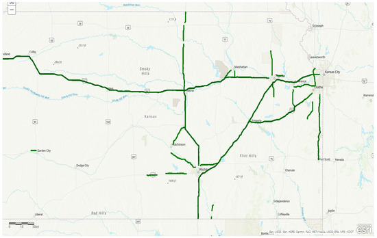
Figure 2.
Locations of treated and non-treated sections.
Figure 2 contains two parts, the first part presenting non-treated sections that were not influenced by a speed limit increase and the second part showing treated sections that were subject to a speed limit increase. The total mileage for non-treated sections is around 300 miles, while the total mileage of treated sections is about 800 miles. Some additional information including the number of curves, International Roughness Index (IRI), side friction, percentage of heavy vehicle (PHV), rural/urban areas, and cross slope related to both treated and non-treated groups in the after the period are summarized in Table 1 and Table 2.

Table 1.
Percentage of heavy vehicle (PHV), area type, cross slope, presence of curve, and International Roughness Index (IRI) for non-treated sites in the after period.
Table 2.
PHV, area type, cross slope, presence of curve, and IRI for treated sites in the after period.
The details of fatal, injury, and PDO crashes for treated sections and non-treated sections are also plotted in the Figure 3.
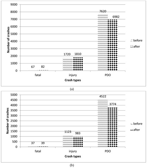
Figure 3.
Observed crashes for treated and non-treated sites during before/after periods. (a) Fatal, Injury, and property damage only (PDO) crashes for treated sections in the before and after periods; (b) Fatal, Injury, and PDO crashes for non-treated sections in the before and after periods.
According to Figure 3, the number of fatal crashes for both treated and non-treated sites have increased. The rate of fatal crashes increased most significantly in treated sites, which experienced an increase in the speed limit. Furthermore, the number of PDO crashes for both treated and non-treated sites have decreased but PDO crashes decreased at a faster rate in non-treated sites, which did not experience an increase in the speed limit. Moreover, the injury crashes for treated sites have increased by 5.2%, while the injury crashes for non-treated sites have decreased by 12.4%, which shows that injury crashes are related to speed limit increase.
3. Methodology
To evaluate the effectiveness of traffic safety after a certain treatment is implemented, the most common method is a before-and-after study [11], which compares the number of crashes in the before-period of a treatment implementation against the after-period. The appropriate comparison group is very important, as it contains non-treated sections that have mutual and comparable features in traffic volume, geometric characteristics, and other section characteristics to the treated sections [12]. Once the comparison group is identified, crash and traffic volume data are required for the same time periods as those considered for the treated group.
In order to evaluate the safety effectiveness of the speed limit increase, the observational before-and-after evaluation studies, using the comparison group method, is applied in this study, as it considers both sections with speed limit change and sections without speed limit change. Using this method, the comparison group (non-treated group) plays a significant role in the before-and-after study, since it estimates the change in crash frequency that has happened in the treated group if no treatment had been made. The comparison group is applied as a control for the trend in crash frequency; its reasons may be unknown, although those factors could be related to the crash frequency and crash severity for both treated and non-treated groups equally. On the other hand, the comparison group is also applied to the control for regression to the mean (RTM) phenomenon [3].
According to the Highway Safety Manual [3], the comparison group method uses SPF(s) as the EB method does, but the SPF(s) are advantageous in computing adjustment factors for non-linear change effects in traffic volumes between before and after periods.
Crash Modification Factor (CMF)
A crash modification factor (CMF) is a multiplicative factor used to estimate the change in the expected (average) number of crashes at a site after a treatment implementation. It is the ratio of the expected number of crashes after the change is implemented to the expected number of crashes if the change is not implemented at the same geographic location. It is also equivalent to the odds ratio (OR) and is computed according to the following Equation [4]:
where,
- = number of crashes in the treated group in year t
- = number of crashes in the treated group in year t − 1
- = number of crashes in the comparison group in year t
- = number of crashes in the comparison group in year t − 1
CMF is a positive value, so the lower limit is zero and there is no upper limit for a CMF, so it may theoretically take values up to infinity. A CMF value of one indicates that the expected number of crashes with the change is equivalent to the expected number of crashes without the change, which means that the treatment has had no effect on safety. Similarly, a CMF less than one shows that the treatment has had a safety benefit, while a CMF greater than one means the treatment has had a negative effect on safety [13].
Detailed procedures for performing an observational before/after study with the comparison group method is presented in the following steps [3].
Step 1: The predicted crash frequency is calculated for treated sites during each year of the before and after periods [14]. In this step, the correct safety performance function (SPF) should be utilized. The freeway SPF for computation according to HSM is as follows:
With,
where,
- = predicted average multiple vehicle crash frequency (mv) or single vehicle crash frequency (sv) of a freeway segment (fs) with base conditions, n lanes, and severity z (z = fi: fatal and injury, PDO) (crashes per year).
- = effective length of freeway segment (mi)
- = length of freeway segment (mi)
- = length of ramp entrance i adjacent to subject freeway segment (mi)
- = length of ramp exit i adjacent to subject freeway segment (mi)
- = Annual Average Daily Traffic volume of freeway segment (veh/day); and
- a, b, c = regression coefficients
As all of the treated sites are 4 lane freeways, a, b, and c coefficients are according to tables 18-5 and 18-7 in HSM.
Step 2: The predicted average crash frequency is calculated for each comparison site (non-treated site) in the before and after period, and the SPF is based on the site characteristics. There are two different facility types for comparison group sites. Some sites are freeways and the others are rural 4-lane divided highways (non-interstate sections). Two different SPFs should, therefore, be used. The SPF for freeways is identical to the treated sites, while the SPF is based on the Highway Safety Manual for the rural multi-lane highways as follows:
where,
- = predicted average crash frequency for divided multi-lane highway segment
- AADT = Annual Average Daily Traffic (vehicles/day) on multi-lane highway segment
- L = multi-lane highway segment length (miles)
- a, b = regression coefficients
The regression coefficients for multi-lane highways are selected from table 11-5 of the HSM based on total crashes or fatal and injury crashes.
Step 3: The adjustment factor of treated sites in the before period is calculated for each of the non-treated sites in the before period using the equation as follow:
where,
- = sum of predicted average crash frequencies at treatment site in the before period using the appropriate SPF and AADT.
- = sum of predicted average crash frequencies at comparison site j in the before period using the correct SPF and specific AADT.
- = years of before period for treatment site
- = years of before period for comparison site ϳ
Step 4: The adjustment factor of treated sites in the after period is calculated for each of the comparison sites in the after period using the following equation:
where,
= sum of predicted average crash frequencies at treatment site in the after period using the appropriate SPF and AADT.
sum of predicted average crash frequencies at comparison site j in the after period using the correct SPF and specific AADT.
Step 5: The expected crash frequency is calculated in the before period ( for an individual comparison site using the following equation:
Step 6: The expected crash frequency is calculated in the after period ( for an individual comparison site using the following equation:
Step 7: The summation of expected crash frequencies in the before period and after period is calculated for each treated site and comparison site.
Step 8: For each of the treated sites, the comparison ratio of the comparison group is calculated by using the following equation:
Step 9: The expected average crash frequency for each of the treated sites without any treatment in the after period is calculated by the equation as follow:
where,
= Number of observed crashes for treated sites in the before period
Step 10: The safety effectiveness, expressed as an odds ratio () at an individual treatment site i is calculated by using the following equation:
where,
= Number of observed crashes for treated sites in the after period
Step 11: The log odds ratio (R) for each of the treated sites is calculated using the following equation:
Step 12: The weighted adjustment factor () is calculated for each of the treated sites as follows:
where,
= + + +
Step 13: The weighted average log odds ratio (R) across all treated sites is calculated by using the following equation:
Step 14: The overall effectiveness of the treatment expressed as an odds ratio or CMF, averaged across all treated sites is estimated as follows:
where,
R = weighted average log odds ratio across all of the treated sites
Step 15: The overall safety effectiveness index ( is expressed as the percentage of change in crashes across all treated sites as follows:
where,
OR = overall crash modification factor (CMF) across all of the treated sites
Step 16: The standard error of treatment effectiveness is computed in order to measure the precision of the treatment effectiveness by using the following equation:
where,
= total weighted adjustment factor across all of the treated sites
Step 17: The statistical significance of estimated safety effectiveness is assessed by making comparisons with the measure of Abs ( and drawing conclusions based on the following criteria (11):
- If Abs ( < 1.7, treatment effect is not significant at 90% confidence level.
- If Abs ( ≥ 1.7, treatment effect is significant at 90% confidence level.
- If Abs ( ≥ 2, treatment effect is significant at 95% confidence level.
4. Data Analysis and Results
Based on the steps listed in the methodology section, all sites should be involved in calculations in order to estimate the CMF. For this purpose, some sample calculations for the first treated sites and non-treated sites are provided in Table 3 based on two different crash types, and the same procedure is repeated for all remaining sites in order to obtain the final results.
Table 3.
Sample calculations for the first treated and non-treated site in the before-and-after period.
To estimate the CMF for each site, it is necessary to have the observed crashes in the after-period and the expected crashes in the after-period without treatment for each site. Table 4 presents these results.
Table 4.
Expected and observed total crashes and fatal plus injury crashes for treated sites.
By dividing the expected crashes in the after-period without treatment by the observed crashes in the after-period, the CMF is identified for each treated site according to total crashes and fatal, and injury crashes. Finally, the CMF results of each site is tabulated in Table 5 for fatal and injury crashes and total crashes separately.
Table 5.
CMF of total crashes and fatal and injury crashes for each treated sites.
According to Table 5, the CMF for fatal and injury crashes has increased at a faster rate than the CMF for total crashes. For example, the CMF for fatal and injury crashes for site numbers 14, 22, 37, and 38 doubled that of other sections. Meanwhile, site number 38 is the only site which shows a significant increase in the CMF for total crashes.
In order to determine the overall CMF, it is necessary to compute the weighted average log odds ratio (R) across all of the treated sites, according to Equation (14) and as explained in the methodology section. When the R-value is known, the overall CMF can be easily estimated according to Equation (15) in the methodology section.
The combined computation results, for the overall CMF based on total crashes, and fatal and injury crashes, are summarized in Table 6. Moreover, the statistical significance results at 95% confidence level, which is commonly used in statistical estimations, is also specified separately in the table for both fatal and injury crashes and total crashes. Additionally, Table 6 presents the weighted average log odds ratio (R) and standard error of treatment effectiveness for both fatal and injury crashes, and total crashes.
Table 6.
Combined computation results based on total crashes and fatal and injury crashes.
All the computations included in Table 4 are presented for all treated sites because the goal is to estimate the overall CMF across all treated sections together. Likewise, the ultimate objective is to find the percent increase of fatal and injury crashes, and of total crashes.
When the before-and-after analysis with the comparison group method was applied, there was a 27% increase for total crashes. Additionally, the separate analysis carried out for fatal and injury crashes showed a nearly 35% increase, which is 8% more than the increase in total crashes, and these increases were both statistically significant at 95% confidence level.
5. Discussion
The results from this analysis show that raising the speed limits resulted in an increase in total crashes, as well as fatal and injury crashes. Furthermore, the treatment effect is statistically significant at 95% confidence level, since the Abs () is greater than 2 according to step 17 in the methodology section, which is 13.80 for total crashes and 7.49 for fatal plus injury crashes. Fatal and injury crashes increased by approximately 8% more than total crashes, which shows that the crash severity has become worse after the speed limit change. There are some multi-lane highway sections where the speed limit remained unchanged. However, all the sections that received a speed limit change are freeways, which need specific SPF(s) for identifying the predicted crash frequency [15].
Many people believe that raising the speed limit is beneficial as it saves costs and causes travel- time reduction. However, the life losses from fatal and injury crashes due to speed limit changes is equivalent to the years saved from decreased travel time [16].
Furthermore, raising the speed limit on some road sections could rise the acceptability of higher speeds by both the driving public and law enforcement, which could lead to the “spillover” impact. Ultimately, increasing the speed limit on some roads but not all other similar roads may change traffic flow from the roads with low-speed to the roads with high-speed [17]. In this study, there were no available calibration factors for Kansas. The SPF(s) used in this study are ideal for calibrating and using specifically for the state of Kansas rather than utilizing the SPF provided in HSM. The EB method would also be applicable for later use in this study since the number of crashes in the comparison group is lower than the treated group [18]. Likewise, it would be interesting to see how the total number of crashes, and fatal and injury crashes, can be compared for the same locations, during the before-and-after speed limit increase. It would also be useful to conduct a speed study to compare the speed of vehicles in the before-period and the speed of vehicles after a limit increase, in order to evaluate whether the changes in operating speeds have been statistically significant or not [19]. Likewise, it would be useful to evaluate the speed study based on the availability of speed data according to automatic traffic recorders (ATRs), located on different sections of freeways that receive a speed limit increase, and sections without an increase, in order to identify if there is any behavior change after a speed limit increase.
6. Conclusions
This study depicts that the speed limit increase from 70 mph to 75 mph resulted in a 27% increase in the total number of crashes that had occurred on freeway sections in Kansas. Moreover, the number of fatal and injury crashes had the most significant increase, which was approximately 35% at the locations that received a speed limit change. Overall, the speed limit increase in Kansas has contributed to a deterioration of safety by affecting the number and severity of crashes, which were both found to be statistically significant at 95% confidence level. Future research will examine the drivers’ average speed during the before-period and compare it to the average speed after a limit change to understand whether drivers alter their behavior or not.
Author Contributions
S.D. wrote the proposal for the project and received the funding to conduct the research. The analysis was developed by R.S. who also wrote the first draft of the manuscript. A.J.A and D.D.Y helped for English check revision and contributing to address the reviewers’ comments precisely. Overall, all authors contributed to the final version of the manuscript.
Funding
This project was supported by K-TRAN program of the Kansas Department of Transportation. The writers wish to acknowledge the assistance provided by the project monitor, Mr. Steven Buckley. The authors also wish to thank Mrs. Tina Cramer for providing the data needed to conduct this study.
Conflicts of Interest
The authors declare no conflicts of interest.
References
- Kansas Legislature Conference Committee. Kansas to Raise Rural Interstate Speed Limits to 75 MPH. 2011. Available online: www.thenewspaper.com/news/34/3448.asp (accessed on 29 May 2017).
- National Transportation Safety Board. Reducing Speeding-Related Crashes Involving Passenger Vehicles; Safety Study NTSB/SS-17/01; National Transportation Safety Board: Washington, DC, USA, 2017.
- AASHTO. Highway Safety Manual; American Association of State Transportation Officials: Washington, DC, USA, 2014; Volume 1. [Google Scholar]
- De Pauw, E.; Daniels, S.; Thierie, M.; Brijs, T. Safety effects of reducing the speed limit from 90km/h to 70km/h. Accid. Anal. Prev. 2014, 62, 426–431. [Google Scholar] [CrossRef] [PubMed]
- Elvik, R. A before–after study of the effects on safety of environmental speed limits in the city of Oslo, Norway. Saf. Sci. 2013, 55, 10–16. [Google Scholar] [CrossRef]
- Renski, H.; Khattak, A.; Council, F. Effect of speed limit increases on crash injury severity: Analysis of single-vehicle crashes on North Carolina interstate highways. Transp. Res. Rec. J. Transp. Res. Board 1999, 1665, 100–108. [Google Scholar] [CrossRef]
- Rock, S.M. Impact of the 65mph speed limit on accidents, deaths, and injuries in Illinois. Accid. Anal. Prev. 1995, 27, 207–214. [Google Scholar] [CrossRef]
- Najjar, Y.M.; Stokes, R.W.; Russell, E.R.; Ali, H.E.; Zhang, X. Impact of New Speed Limits on Kansas Highways; K-TRAN Report; Publication K-TRAN: KSU-98-3; Kansas Department of Transportation: Topeka, KS, USA, 2000.
- Ledolter, J.; Chan, K.S. Evaluating the impact of the 65mph maximum speed limit on Iowa rural interstates. Am. Stat. 1996, 50, 79–85. [Google Scholar]
- Høye, A. Safety effects of section control-An empirical Bayes evaluation. Accid. Anal. Prev. 2015, 74, 169–178. [Google Scholar] [CrossRef] [PubMed]
- Elvik, R. The importance of confounding in observational before-and-after studies of road safety measures. Accid. Anal. Prev. 2002, 34, 631–635. [Google Scholar] [CrossRef]
- Persaud, B.; Lyon, C. Empirical Bayes before–after safety studies: Lessons learned from two decades of experience and future directions. Accid. Anal. Prev. 2007, 39, 546–555. [Google Scholar] [CrossRef] [PubMed]
- Gayah, V.; Vikash, V.; Donnell, E.T. Establishing Crash Modification Factors and Their Use; Final Report, FHWA, Publication FHWA-PA-2014-005; Pennsylvania Department of Transportation: Harrisburg, PA, USA; Pennsylvania State University: State College, PA, USA, 2014. [Google Scholar]
- Griffith, M. Safety evaluation of rolled-in continuous shoulder rumble strips installed on freeways. Transp. Res. Rec. J. Transp. Res. Board 1999, 1665, 28–34. [Google Scholar] [CrossRef]
- Brimley, B.; Saito, M.; Schultz, G. Calibration of Highway Safety Manual safety performance function: Development of new models for rural two-lane two-way highways. Transp. Res. Rec. J. Transp. Res. Board 2012, 2279, 82–89. [Google Scholar] [CrossRef]
- Miller, T.R. 65 MPH: Winners and Losers; Final Grant Report, Publication U.I. Project 3807, HS-807 451; The Urban Institute: Washington, DC, USA, 1989. [Google Scholar]
- Wagenaar, A.C.; Streff, F.M.; Schultz, R.H. Effects of the 65mph speed limit on injury morbidity and mortality. Accid. Anal. Prev. 1990, 22, 571–585. [Google Scholar] [CrossRef]
- Montella, A. Safety evaluation of curve delineation improvements: Empirical Bayes observational before-and-after study. Transp. Res. Rec. J. Transp. Res. Board 2009, 2103, 69–79. [Google Scholar] [CrossRef]
- Jernigan, J.D.; Strong, S.E.; Lynn, C.W. Impact of the 65 MPH Speed Limit on Virginia’s Rural Interstate Highways; Final Report; Publication VTRC 95-R7; Virginia Transportation Research Council: Charlottesville, VA, USA; Virginia Department of Transportation: Richmond, VA, USA, 1994. [Google Scholar]
© 2018 by the authors. Licensee MDPI, Basel, Switzerland. This article is an open access article distributed under the terms and conditions of the Creative Commons Attribution (CC BY) license (http://creativecommons.org/licenses/by/4.0/).