Kū Hou Kuapā: Cultural Restoration Improves Water Budget and Water Quality Dynamics in Heʻeia Fishpond

Abstract

In Hawaiʻi, the transition from customary subsistence flooded taro agroecosystems, which regulate stream discharge rate trapping sediment and nutrients, to a plantation-style economy (c. the 1840s) led to nearshore sediment deposition—smothering coral reefs and destroying adjacent coastal fisheries and customary fishpond mariculture. To mitigate sediment transport, Rhizophora mangle was introduced in estuaries across Hawaiʻi (c. 1902) further altering fishpond ecosystems. Here, we examine the impact of cultural restoration between 2012–2018 at Heʻeia Fishpond, a 600–800-year-old walled fishpond. Fishpond water quality was assessed by calculating water exchange rates, residence times, salinity distribution, and abundance of microbial indicators prior to and after restoration. We hypothesized that R. mangle removal and concomitant reconstruction of sluice gates would increase mixing and decrease bacterial indicator abundance in the fishpond. We find that Heʻeia Fishpond’s physical environment is primarily tidally driven; wind forcing and river water volume flux are secondary drivers. Post-restoration, two sluice gates in the northeastern region account for >80% of relative water volume flux in the fishpond. Increase in water volume flux exchange rates during spring and neap tide and shorter minimum water residence time corresponded with the reconstruction of a partially obstructed 56 m gap together with the installation of an additional sluice gate in the fishpond wall. Lower mean salinities post-restoration suggests that increased freshwater water volume influx due to R. mangle removal. Spatial distribution of microbial bio-indicator species was inversely correlated with salinity. Average abundance of Enterococcus and Bacteroidales did not significantly change after restoration efforts, however, average abundance of a biomarker specific to birds nesting in the mangroves decreased significantly after restoration. This study demonstrates the positive impact of biocultural restoration regimes on water volume flux into and out of the fishpond, as well as water quality parameters, encouraging the prospect of revitalizing this and other culturally and economically significant sites for sustainable aquaculture in the future.

1. Introduction

1.1. Native Hawaiian Fishpond Mariculture and Food Security

As the catch rate of our global fisheries levels off due to degradation of the environment and collapse of specific fish populations, the demand for aquaculture production of fish is projected to increase markedly [1]. Concerns over sustainable food production have brought indigenous models of resource management to the fore. Hawaiʻi currently imports about half of our seafood [2] and local aquaculture is estimated to supply only ~20,000 lbs (9072 kgs) annually [3], but this was not always the case. For centuries, Native Hawaiians developed marine aquaculture that utilized natural enrichments via freshwater from surface and submarine groundwater discharge in managed estuaries, called loko iʻa (fishponds) [4]. Loko iʻa kuapā (walled fishponds) were intentionally built in natural embayments at the interface of freshwater streams and the ocean where nutrients from streams promoted the growth of primary producers in constrained brackish ecosystems. The kuapā (walls) regulates freshwater inflow to mākāhā (size-slotted sluice gates), creates a low wave energy environment within the loko iʻa, impedes water volume flux into and out of the loko iʻa and ensures that a minimum volume of water is retained in the loko iʻa at all times, especially at extremely low tides. Where water volume flux (m³ s⁻¹) is the volume of water passing through each mākāhā over time. Water volume flux can be in to or out of the loko iʻa, depending on mākāhā, tidal stage and other environmental conditions. In this system, unicellular photosynthetic microbes form the base of a complex food web that yield energetically efficient protein production of crustaceans and herbivorous fish species. Kiaʻi loko iʻa (fishpond stewards) practiced stock enhancement, leveraging knowledge of juvenile fish migration to trap target species behind mākāhā until reaching maturity and preventing entry of large predators. In addition, kiaʻi loko regulate water volume flux or harvest fish by blocking mākāhā. It is estimated that loko iʻa in Hawaiʻi could have yielded approximately 2 million pounds of fish per year total historically [5,6].

1.2. The Legacy of Land Use Change and Invasive Species on loko iʻa

Physical changes (development, disuse, sedimentation, storm damage) and biological invasions have dramatically altered many loko iʻa. Beginning in the 1800s, a shift from subsistence to plantation economy led to erosion and siltation of the nearshore environment. In an attempt to mitigate and stabilize these impacts, mangroves were introduced to Hawaiʻi in 1902 [7]. Mangroves are highly appreciated in their native habitats for the ecosystem services they provide: shoreline protection and sediment stabilization [8], litterfall subsidy [9] and provision of nursery grounds [8]. Thus, by modifying their environment, mangroves have cascading effects for resident biota, acting as important ecosystem engineers.

However, in Hawaiʻi, mangroves have caused a variety of negative ecological and economic impacts that motivate their removal [10]. Mangrove’s preference for halotypic ecotones favor their growth in estuaries with their root systems obstructing mākāhā, decreasing water volume flux, flushing, and circulation of loko iʻa and the streams that feed them [11,12,13]. Instead of sandy habitats, mangrove vegetated areas have high sedimentation rates and anoxic sediments due to bacterial decomposition of mangrove leaf detritus [11,14]. Moreover, mangrove drawdown of nitrogen and phosphate and decrease dissolved oxygen from overlying waters, potentially inhibiting primary production rates in loko iʻa [13]. Importantly, the absence of mangrove feeding specialists in Hawaiʻi has resulted in the poor assimilation of mangrove-derived nutrients from introduced stands [15] because detritivores native to Hawaiʻi are not adapted to utilizing mangrove detritus, which tends to be tannin-rich and nitrogen-poor [16].

Post-World War II, a combination of urbanization, the introduction of invasive species, stochastic events (e.g., storms, floods, tsunamis and lava flows) led to deterioration of loko iʻa across the state [6]. By 1977, only 28 loko iʻa were still in production, and by 1985, merely 7 loko iʻa were in commercial or subsistence use [6]. The loss of actively maintained loko iʻa exacerbated the spread of invasive mangrove in coastal estuaries [17].

1.3. Revitilization of loko iʻa: Heʻeia Fishpond as a Model

Driven by a desire to re-establish customary practices, provide economic opportunities to local communities and improve production of crustaceans and herbivorous fish, a grassroots movement of loko iʻa restoration has gained momentum since the early 2000s [18,19,20]. Hui Malama Loko Iʻa is a statewide network of indigenous kiaʻi loko dedicated to restoring loko iʻa for food production [21]. Loko iʻa restoration generally entails mangrove removal and dry stacking of basalt with coral/rubble internally. Typical mangrove clearing practices in Hawaiʻi include the removal of the above-sediment mangrove biomass, leaving intact the prop roots and the root-fiber mat within the sediment. Despite increased loko iʻa restoration across the state, we know of no published data on the effects of mangrove removal and loko iʻa infrastructure repair on water circulation dynamics and water quality.

Located on the windward side of Oʻahu Island, Hawaiʻi (Figure 1A), Heʻeia Fishpond (also known as Pihi Loko Iʻa) is a loko iʻa kuapā estimated to have been built 600-800 years ago atop the Malaukaʻa fringing reef [22] and has been at the forefront of loko iʻa restoration in Hawaiʻi. Rhizophora mangle was introduced to the Heʻeia estuary in 1922 to control runoff from upstream agriculture and stabilize sediments [11,15]. The circulation and water volume flux patterns within Heʻeia Fishpond were compromised during the Keapuka Flood, which occurred in 1965. The highest discharge rate on record from Haʻikū and ʻIolekaʻa streams occurred during the Keapuka Flood [23] on May 2, 1965. Flood waters first broke the kuapā in the northwestern sector adjacent to Heʻeia Stream, creating a 183 m opening in the loko iʻa. Historical tidal data [24] indicate that the flood likely occurred during a perigean spring tide (a. k. a. King Tide), thus the 56 m break in the kuapā on eastern seaward side as well (Figure 1B, “Ocean Break”) likely resulted from build-up of internal pressure within the loko iʻa coupled with an extremely low tide outside the loko iʻa.

As a result of the shift from a constrained to a radically unconstrained system, the fundamental functioning of the loko iʻa has changed: the volume became strongly tidally dominated and fish production using customary mariculture techniques could no longer be practiced. A dense mangrove forest around the mouth of Heʻeia stream expanded into the loko iʻa, growing along and eventually obscuring the kuapā and effectively decreasing the amount of water exchange. Sediment loading from Heʻeia Stream, agriculture and urbanization overwhelmed the original mechanisms by which material was flushed out of the loko iʻa [25]. The average loko iʻa depth is ~1 m, due to progressive accumulation of terrigenous particulates on the coral benthos, accelerated by a dense mangrove root mass [26]. Increased salinity, organic matter, and turbidity may have facilitated a shift in the biological diversity and composition of the loko iʻa away from desirable aquaculture species and toward invasive macroalgae.

Though limited kuapā repair over the last 25 years has enabled conventional net pen aquaculture in the loko iʻa, the ecosystem became steadily more eutrophic. In 1988, Mark Brooks leased the property, installing a 0.9 m retaining wall of cement cinder blocks in Ocean Break that reduced the tidal influence and prevented water exchange except at spring tides (Figure 1C). In addition, a previous flood in 1927 deposited a portion of the kuapā into the interior of the loko iʻa creating a mangrove stand where introduced cattle egrets (Bubulcus ibis) established a rookery (Figure 1B). In 2017 an estimated 2000–3000 cattle egrets dwelled in this mangrove stand. The potential for human and animal health impacts from microbial contamination is a central concern in maintaining an ecologically balanced and productive loko iʻa [27,28]. Limited circulation within Heʻeia exacerbates this issue, particularly given the rich source of guano and nutrients produced by the egret colony.

Since 2001, the Native Hawaiian non-profit organization Paepae o Heʻeia has sought to foster cultural sustainability and restore and maintain a thriving loko iʻa for the local community by linking traditional knowledge and contemporary management practices. As the compromised mākāhā system made regulation of fish migration and recruitment impossible, Paepae o Heʻeia initially centered their aquaculture activities around high-density cultivation in quarter-acre net pens. From 2006–2009 Paepae o Heʻeia produced approximately 1.2 metric tons of Pacific threadfin. However two events massive fish mortality events in 2009, prompted a re-evaluation of the use of conventional rearing techniques in Heʻeia Fishpond. Repairing the kuapā would eliminate the need for net pen aquaculture, enabling fish stock to move throughout the entire loko iʻa toward cooler and/or more oxygenated areas in response to future environmental stress. Paepae o Heʻeia hypothesized that consistent freshwater input and nutrients, via functional mākāhā would increase primary productivity and subsequently increase the biomass of native herbivores in the loko iʻa.

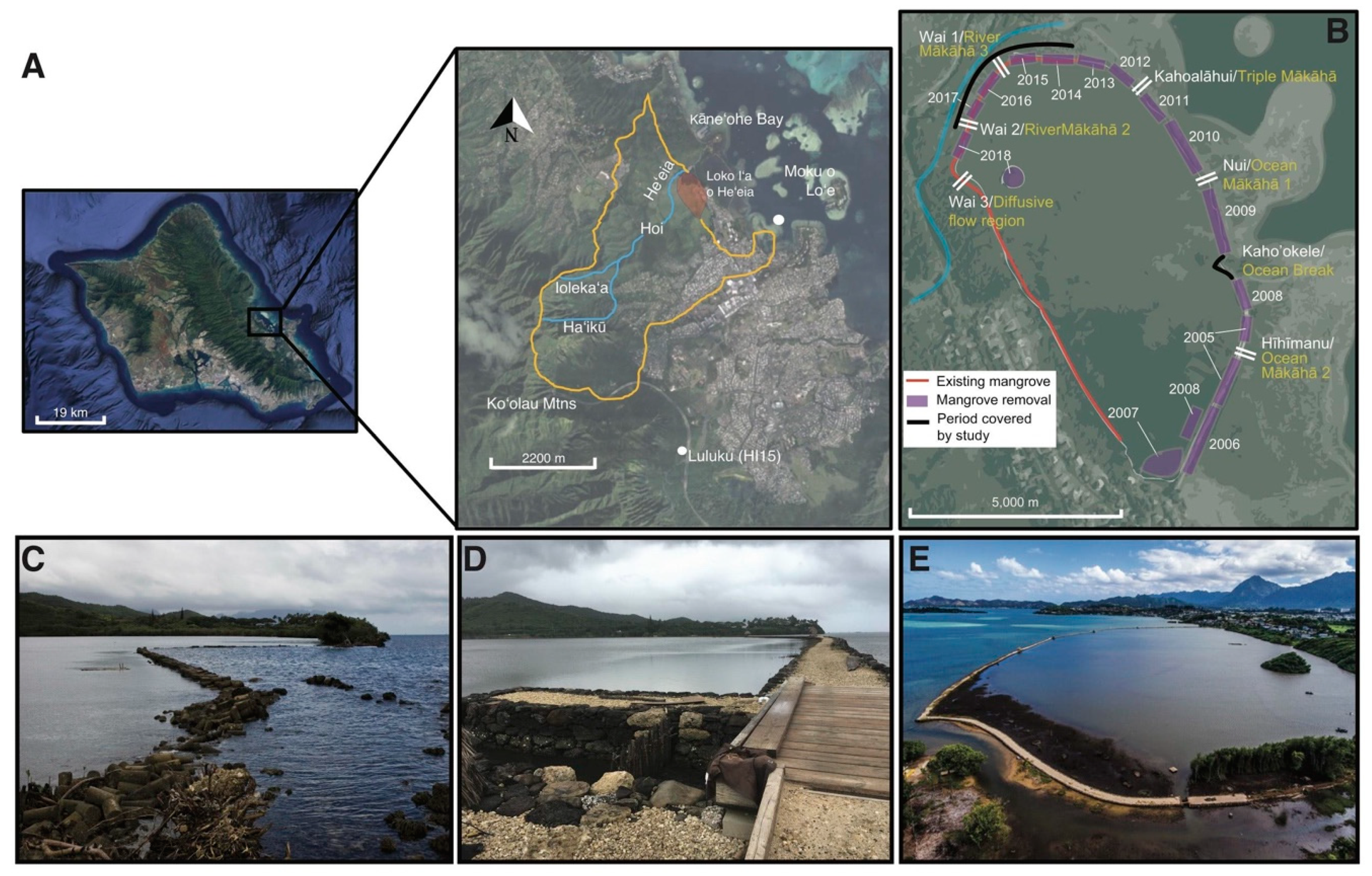
1.4. Biocultural Restoration of Heʻeia Fishpond: 2012–2018

Biocultural restoration from 2012 to 2018 targeted two areas: the gap in the seaward kuapā and the section bordering Heʻeia Stream (Figure 1B). The restoration phase involving repair of the 56 m kuapā gap (Ocean Break) spanned 2014–2015 and was known as Pani ka puka (Shut the door). Kiaʻi loko used traditional external materials (pohaku pele, basalt rock) and a mix of traditional and contemporary internal materials (koʻa, coral rubble, and remnant cinder blocks) to coordinate rebuilding of the north and south segments of the broken kuapā to meet in the middle. Rather than rebuild a continuous kuapā spanning the entire seaward side, Paepae o Heʻeia elected to install a new mākāhā (Kahoʻokele) to increase loko iʻa circulation, increase oxygenation of the water column, and promote recruitment of marine species (Figure 1C,D). Mākāhā site selection was based on empirical kiaʻi loko observations of areas with the highest abundance and diversity of marine life (e.g., fish, oysters, macroalgae, sponges).

With the help of over 50,000 community volunteers, Paepae o Heʻeia has resurrected over 2 km of kuapā along its historical footprint and progressively removed invasive R. mangle (Figure 1B–E). Historically, the volume and location of surface water input into Heʻeia Fishpond from the Hoi wetland and Heʻeia Stream was confined to water volume flux through mākāhā. After the 1965 Keapuka flood, however, damage to the kuapā and subsequent R. mangle growth resulted in an attenuated and diffuse flow of fresh water into the loko iʻa. Over this period of this study, Paepae o Heʻeia commenced kuapā restoration along Heʻeia Stream and concomitant mangrove removal (Figure 1E) in order to alter the path of surface water into the loko iʻa. Kiaʻi loko posited that restoring the wall and mākāhā would increase the rate of water exchange and flow rate, which might improve fish passage into the estuary. R. mangle was initially removed from the remnant kuapā and nearby loko iʻa interior by clear-cutting and incineration on site. With the exception of 2014–2015, the mean rate of restoration was 154.84 ± 17.33 m year⁻¹, totaling 619.35 m kuapā (Table S1).

In the present study, we partnered with Paepae o Heʻeia, kiaʻi loko of Heʻeia Fishpond, to assess the impacts of restoration from 2012–2018. We have addressed the following questions: (1) How does kuapā infrastructure repair, including mangrove clearance around the loko iʻa periphery, affect circulation dynamics in Heʻeia Fishpond? (2) How does the potential for increased freshwater and ocean water volume flux alter the overall salinity distribution in the loko iʻa? and (3) How do these changes in the physical characteristics of water in the loko iʻa alter microbial bioindicators for fecal contamination?

2. Methods and Materials

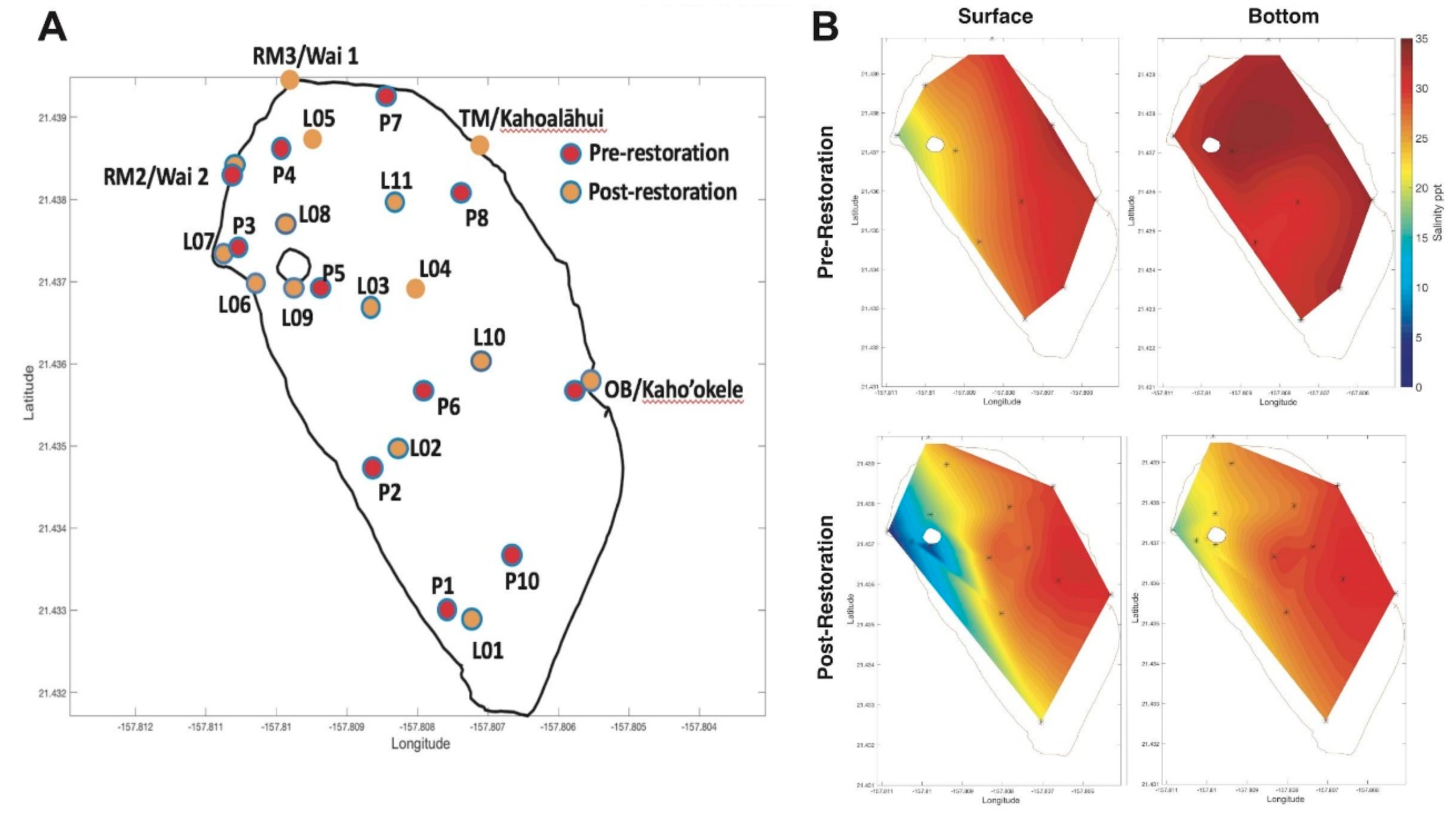
2.1. Study Site

Heʻeia Fishpond (21°26′10.74″ N, 157°48′28.05″W) is a 0.356 km² embayment located on the windward side of Oʻahu Island, Hawaiʻi (Figure 1A). The loko iʻa is completely enclosed by 2.5 km of kuapā and is bordered by Kāneʻohe Bay to the south and east, Heʻeia Stream to the north, and a remnant irrigation ditch (auwai) running longitudinally along its entire west bank. The Haʻikū Stream near the ridgeline of the Koʻolau Mountains converges with the ʻIolekaʻa Stream and becomes Heʻeia Stream before entering the Hoi wetland. Within the Hoi wetlands, a portion of Heʻeia Stream is diverted through a network of auwai, irrigating taro patches. At the terminus of the watershed, Heʻeia Stream historically splits, either flowing south in the auwai that parallels Heʻeia Fishpond or east toward Kāneʻohe Bay. A forest of R. mangle occupies the northwest and western periphery of Heʻeia Fishpond.

Mākāhā are interspersed along the kuapā, connecting the loko iʻa to exterior water sources and regulating surface and seawater exchange with the loko iʻa (Figure 1B,

Table 1. Mākāhā names (post-restoration/pre-restoration), latitude and longitude, compass heading, width (m).

Mākāhā	Latitude	Longitude	Heading	Width (m)
Hīhīmanu/Ocean Mākāhā 2	21.4357389	−157.80531	111°/291°	2.00
Kahoʻokele/Ocean Break	21.4372333	−157.80583	80°/260°	3.05
Nui/Ocean Mākāā 1	21.4384222	−157.80675	63°/243°	6.48
Kahoalāhui Kealohi/Triple Mākāhā 1	21.4396667	−157.80993	48°/228°	1.88
Kahoalāhui Koʻa Mano/Triple Mākāhā 2	21.4396667	−157.80993	48°/228°	1.78
Kahoalāhui Kekepa/Triple Mākāhā 3	21.4396667	−157.80993	48°/228°	1.55
Wai 1/River Mākāhā 3	21.4386034	−157.81072	310°/130°	2.18
Wai 2/River Mākāhā 2	21.4379231	−157.80782	290°/110°	1.85
Diffuse flow region/River Makāhā 1	21.4386583	−157.81077	n/a	n/a

). Hereafter, names of mākāhā follow the convention used by Paepae o Heʻeia in 2018. Designations from previous studies [29,30] are also given. For the past 50 years, mākāhā channels in Heʻeia Fishpond have had concrete floors with vertical walls composed of basalt and coral rubble with either a semi-permeable barrier fence or grid constructed from wood or plastic (Figure 2). With the exception of Kahoʻokele, the floor of the mākāhā are slightly higher than the natural bottom of the loko iʻa. All fieldwork was conducted with the permission of Paepae o Heʻeia and the private landowner, Kamehameha Schools (Joey Char, Land Asset Manager, Kamehameha Schools Community Engagement and Resources Division).

2.2. Water Volume Flux and Volume Change Calculations

To evaluate the current direction (°), water level (m) and water velocity (m s⁻¹) into and out of the loko iʻa, Sontek Argonaut Shallow Water (SW) Profilers (SonTek, San Diego, CA, USA) and battery housings were deployed in each mākāhā for 7 days (Figure 2, Table S1). Each instrument packet was oriented facing into the channel and mounted to 0.7 × 0.7 m metal mooring with ~25 kg weights and placed at the bottom of each mākāhā channel. Measurements were recorded every 20 s with an averaging interval of 10 s. The blanking distance was set to the minimal amount of 0.07 m, as the mean water column was <0.50 m. Over this period, one full neap and spring tide were measured. Water volume flux data and water velocity measurements (m s⁻¹) acquired from the Sontek Argonaut SW Profiler were used to generate rating curves for each mākāhā at (spring flood tide, SF; spring ebb tide, SE; neap flood tide, NF; and neap ebb tide, NE) using the following equation:

φ = wdv

(1)

where φ is the water volume flux, w is the respective mākāhā width (m), d is the water level vector (m) changing over time with the tide, and v is the water velocity (m s⁻¹) through the mākāhā channel [29,30]. Rating curves were fitted using a poly-fit function with a best-fit line and 95% confidence intervals in Matlab (The MathWorks Inc., Natick, MA, USA). To account for bidirectional water flow in the mākāhā due to tidal forcing, water volume flux was determined for an entire tidal cycle at the following tidal stages: SF, SE, NF, and NE. The cycle with the largest tidal amplitude was selected for spring tide, while the cycle with the lowest tidal amplitude was selected for neap tide. The data set was split into flood (from pressure minimum to pressure maximum) and ebb tide (from pressure maximum to pressure minimum) based on tidal stage.

Based on the water volume flux, mean and maximum flow through each mākāhā were calculated for four tidal cycles (SF, SE, NF, NE). Peak water volume flux occurs mid-way between slack tides, thus the water level to water volume flux relationship, the rating curve, typically resembles a “C” curve or vertical sine function. To account for varying tidal cycle length caused by mixed semidiurnal tides in Kāneʻohe Bay, individual mākāhā flow rates were normalized by calculating the total volume of water (m³) moving through a mākāhā channel at a given tidal cycle and the hourly water volume flux rate. Here, water volume flux values for Kahoalāhui/Triple Mākāhā were calculated by tripling the flow measurements at the northernmost mākāhā channel (Kealohi).

Precipitation, tidal state, wind direction, and wind speed were used as criteria for selecting pre- and post-restoration dates for comparison (Table S3). Daily (cm 24 h⁻¹) and cumulative precipitation over 4 days (cm 96 h⁻¹) were obtained from the NOAA Luluku (HI15) rain gauge station [31]. Mean stream streamflow (mean m³ s⁻¹ 24 h⁻¹) was calculated using data from US Geological Survey discharge station (Haʻikū Station #16275000) obtained from [32]. Wind direction and magnitude was determined from automatic weather station Moku o Loʻe (21.4339° N, 157.7881° W), 1.5 km from Heʻeia Fishpond [33]. A sea level gauge with a water temperature probe, located ~ 10 m offshore of the weather station at a depth of ~ 1 m, was used for tidal data [33].

Loko iʻa volume was calculated using 728 bathymetric depth measurements taken in 2007 normalized to mean low low water from a reference HOBO^® water level logger (Onset, Bourne, MA, USA) deployed at an interior site (21.43466° N, W 157.80699° W) that recorded tidal fluctuations during bathymetry mapping [26,34]. In 2018, we redeployed a HOBO^® water level logger at the same location to recollect reference water level data over a 10-day period. The reference pressure data was corrected for atmospheric pressure fluctuations using a second HOBO logger situated on land to record atmospheric pressure fluctuations reference to adjust for differences in tidal amplitude between pre- and post-restoration.

To calculate post-restoration loko iʻa volume, the difference in reference tidal state from pre-restoration (2007) and post-restoration (2018) was applied to the bathymetry dataset at SF, SE, NF, NE tidal states with Station Moku o Loʻe as a reference. A rectangular grid with ~1 m spacing and a natural neighbor interpolation was adopted to estimate depths in between measured bathymetry points in Matlab. For each tidal state, a trapezoidal rule was used with no smoothing applied. The small mangrove island located in the northwest quadrant of the loko iʻa was excluded from our calculations. We assume that there is no change in bathymetry over the course of the study.

To derive minimum residence time in Heʻeia Fishpond, the amount of water exchanged during ebb flood transition was calculated for neap and spring tide using the following equations [30]:

$$\mathsf{\tau }\mathrm{HFS}=\frac{\mathrm{He}ʻ\mathrm{eia} \mathrm{Fishpond} \mathrm{Volume} \mathrm{Exchanged} \left(\mathrm{spring} \mathrm{high} \mathrm{tide}-\mathrm{spring} \mathrm{low} \mathrm{tide}\right)}{\mathrm{He}ʻ\mathrm{eia} \mathrm{Fishpond} \mathrm{Volume} \left(\mathrm{spring} \mathrm{high} \mathrm{tide}\right)}$$

(2)

$$\mathsf{\tau }\mathrm{HFN}=\frac{\mathrm{He}ʻ\mathrm{eia} \mathrm{Fishpond} \mathrm{Volume} \mathrm{Exchanged} \left(\mathrm{neap} \mathrm{high} \mathrm{tide}-\mathrm{neap} \mathrm{low} \mathrm{tide}\right)}{\mathrm{He}ʻ\mathrm{eia} \mathrm{Fishpond} \mathrm{Volume} \left(\mathrm{neap} \mathrm{high} \mathrm{tide}\right)}$$

(3)

where τ_HFS is minimum residence time during spring tide and τ_HFN is minimum residence time during neap tide. To determine residence time, the following assumptions were made: loko iʻa water column is mixed uniformly, all flood and ebb tides are 6 h long, and mākāhā are the only source of water exchange with the following equation:

ϕ^x = 0.01

(4)

where ϕ^x is the percentage of water remaining after 1 flushing cycle (12 h) and x is the residence time in flushing cycles to mix the initial water to a 1% dilution.

2.3. Water Quality Sampling Regime

This study utilized on-going efforts by Nā Kilo Honua o Heʻeia (http://nakilohonuaoheeia.org), a Heʻeia coastal ocean observing research collective at the University of Hawaiʻi at Mānoa that has carried out monthly sampling at Heʻeia Fishpond since 2007 [29]. To minimize the variability of physical and chemical characteristics of the loko iʻa due to tidal exchange, all samples were collected during neap tide over a period of 3–4 h The pre-restoration sampling grid was composed of 10 stations within the loko iʻa, P1−P10, whereas the post-restoration sampling grid was composed of 11 stations within the loko iʻa, L01−L11, and one at each of the mākāhā, M01−M06 (Table S3) Pre-restoration sampling dates in 2014 and post-restoration dates from 2017 were selected to minimize variation in precipitation and stream discharge (Table S4). Reference endmembers for oceanic input were taken outside the kuapā at Kahoʻokele/Ocean Break, E01, whereas endmembers for surface freshwater were collected in Heʻeia Stream between the Hoi wetland and Heʻeia Fishpond outside the kuapā, E02. To minimize the disturbance of the water column and benthos prior to measurements, stations were approached against prevailing currents and winds. Salinity was measured using a YSI Professional Plus (ProPlus) multiparameter sonde (YSI Xylem Brand, Yellow Springs, OH). At each station, a measurement was taken ~ 5–10 cm below the water surface (“surface”) and 5–10 cm above the benthos (“bottom”) by allowing the instrument reading to stabilize for 2–3 minutes before recording values.

Eleven stations were selected for discrete sampling for microbes: Kahoʻokele/Ocean Break, Wai 1, and 9 stations in the loko iʻa interior. Pre-restoration (P01–P10, Ocean Break) and post-restoration (L01–L03, L06–L11, Kahoʻokele, Wai 2) locations differed slightly (Table S4, Figure 5A). At each station, 1L polycarbonate bottles were acid washed and rinsed with ambient surface water three times, before immersion at the surface to fill the bottle completely. Samples were stored at 4 °C and processed within 2 h of collection. Seawater was filtered through a 47 mm diameter, 0.45 μm filter (MCE, Millipore, Sigma, Burlington, MA) and stored at –80 °C prior to DNA extraction.

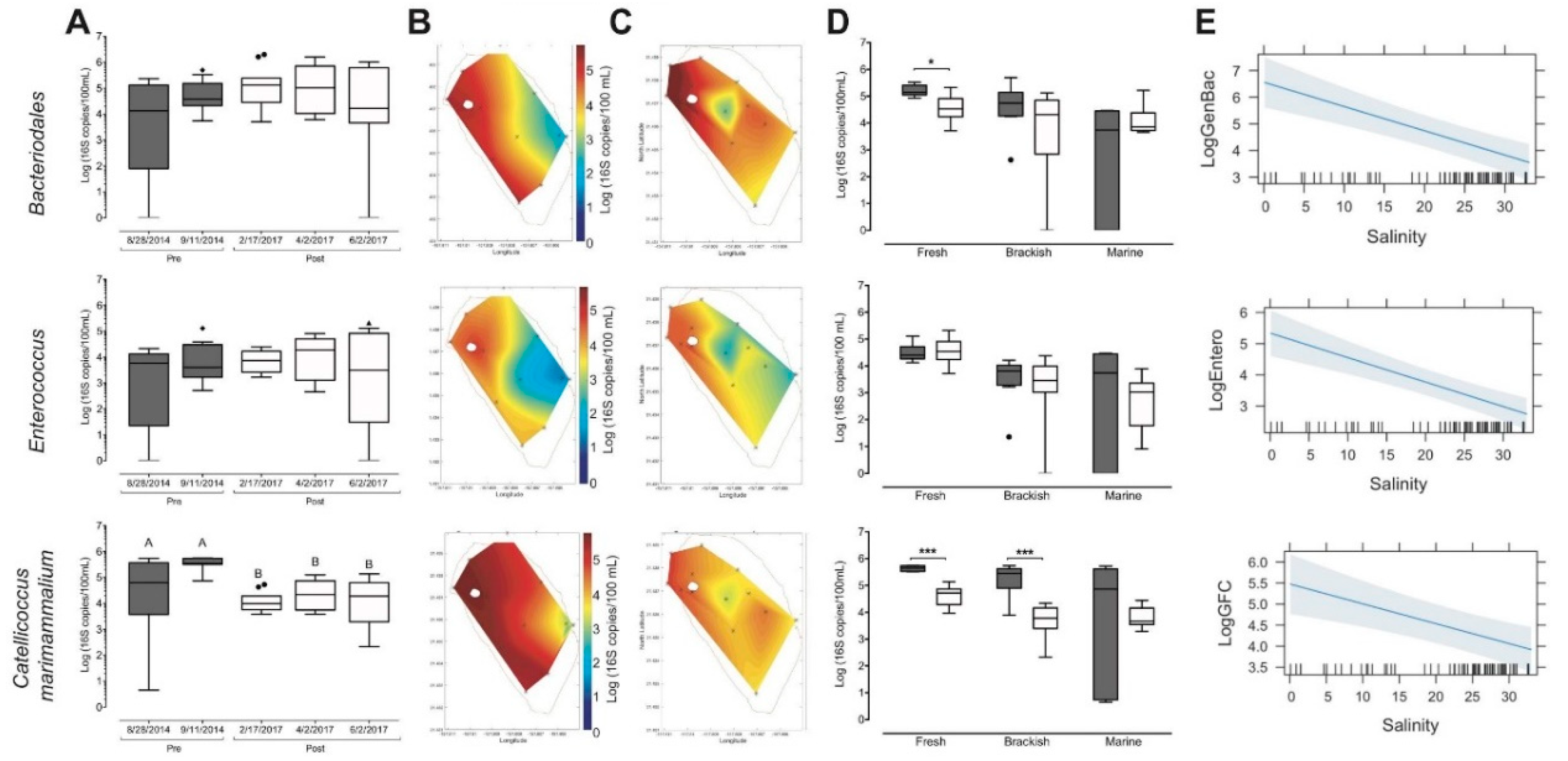
2.4. Microbial Source Tracking

Total genomic DNA (gDNA) was extracted from filters using the PowerWater DNA Extraction kit (QIAGEN, Germantown, MD, USA) following the manufacturer’s instructions. Quantitative PCR (qPCR) was used to determine the abundance of bacterial 16S rRNA genes from mammalian fecal indicator bacteria Enterococcus using assay Entero1a [35,36,37] and Bacteroidales using assay GenBac3 [38,39,40]. Quantification was performed with the KAPA PROBE FORCE qPCR system (Wilmington, MA, USA) using KAPA PROBE FORCE qPCR Master Mix (20 μL reactions), 400 nM specific Taqman primers (

Table 2. The 16S rDNA oligos used in this study.

Target	Primer	Sequence	References
Enteroccocus	Entero1af	AGAAATTCCAAACGAACTTG	[35,36,37]
	Entero1ar	CAGTGCTCTACCTCCATCATT	[35,36,37]
	Entero1ap	6-FAM™/TGGTTCTCT/ZEN™/CCGAAATAGCTTTAGGGCTA/IB®FQ/	[35,36,37]
Bacteroidales	GenBac3f	GGGGTTCTGAGAGGAAGGT	[38,39,40]
	GenBac3r	CCGTCATCCTTCACGCTACT	[38,39,40]
	GenBac3p	6-FAM™/CAATATTCC/ZEN™/TCACTGCTGCCTCCCGTA/IB®FQ/	[38,39,40]
Catellicoccus marimammalium	GFCf	CCC TTG TCG TTA GTT GCC ATC ATT C	[41]
	GFCr	GCC CTC GCG AGT TCG CTG C	[41]

) and template gDNA diluted 1:5. Standards were run in triplicate using an 8-point, 5-fold serial dilution. Cycling parameters for all assays were: 95 °C for 2 min, 45 cycles of 95 °C for 15 s and annealing/extension at 60 °C for 30 s Ct values were converted to concentrations per 100 mL using the manufacturer’s software. The standards used for the Entero1a and GenBac3 assays were genomic DNA extracted from Enterococcus faecalis strain V583 (ATCC^® 700802D-5™) and Bacteroides thetaiotaomicron strain VPI 5482 (ATCC^® 29148™), respectively.

Primers previously shown to detect avian fecal contamination in water [41] were tested on B. ibis fecal DNA (Table 2). Briefly, fecal material was collected from birds present on the small mangrove island on the loko iʻa interior. Total genomic DNA was extracted from avian feces using the DNeasy PowerSoil Kit (QIAGEN, Germantown, MD) following the manufacturer’s instructions. qPCR using GFC primers targeting the 16S rRNA gene from Catellicoccus marimammalium used the KAPA SYBR FAST qPCR system (20 μL reactions), 400 nM primers, and gDNA diluted 1:5. Cycling parameters were as follows: 95 °C for 3 min for enzyme activation, followed by 40 cycles of 95 °C for 3 s and annealing/extension at 60 °C for 20 s Ct values were calculated as previously described with uncultured Catellicoccus sp. 16S rRNA gene, partial sequence (Genbank accession number JN084062) used as a standard.

2.5. Statistics

Statistical significance for pre- and post-restoration events was determined with a pairwise Welch’s t-test to account for differences in variance. Mean baseline events pre-restoration and mean baseline events post-restoration for salinity and log-transformed numbers of microbial biomarker abundance were compared with the t-test for statistical significance in R (R Foundation for Statistical Computing) with the p-value for statistical significance set to p < 0.05. In addition, correlation of GFC/GenBac3/Entero1a distribution with salinity, date, and location was tested using a generalized additive mixed model (GAMM) in R (R Foundation for Statistical Computing). Mean baseline salinity and log-transformed numbers of microbial biomarker abundance pre- and post-restoration was plotted with a contour plot function in Matlab (The MathWorks Inc., Natick, MA, USA).

3. Results

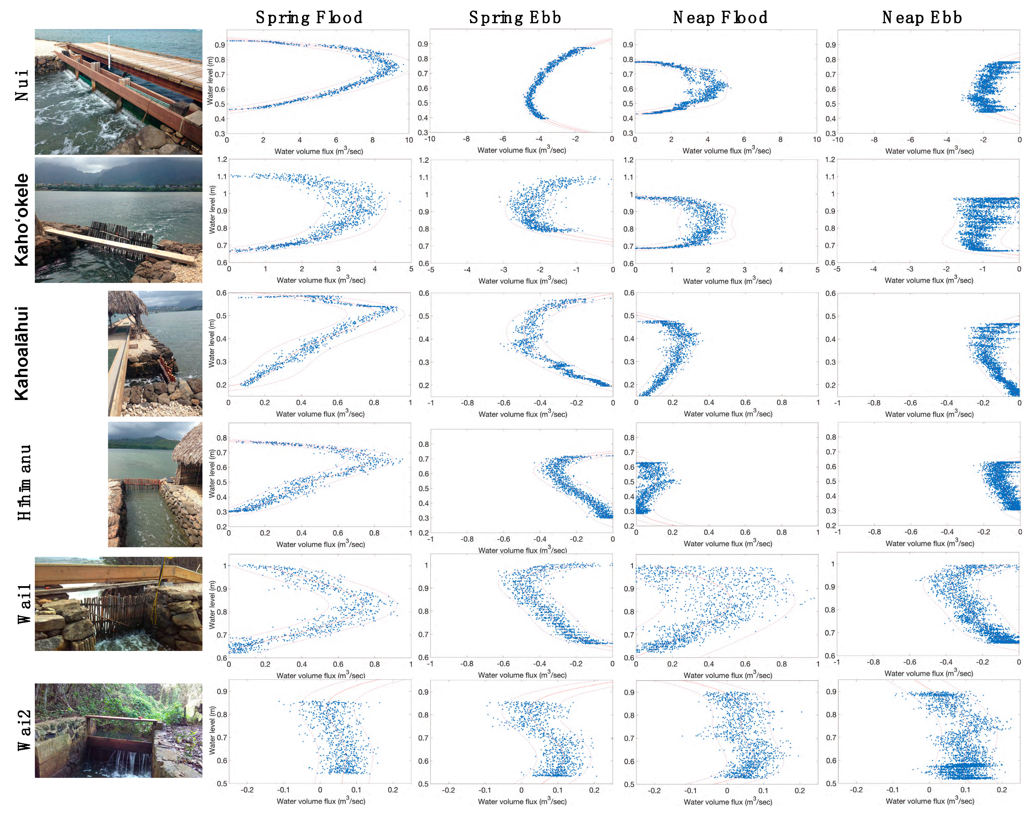
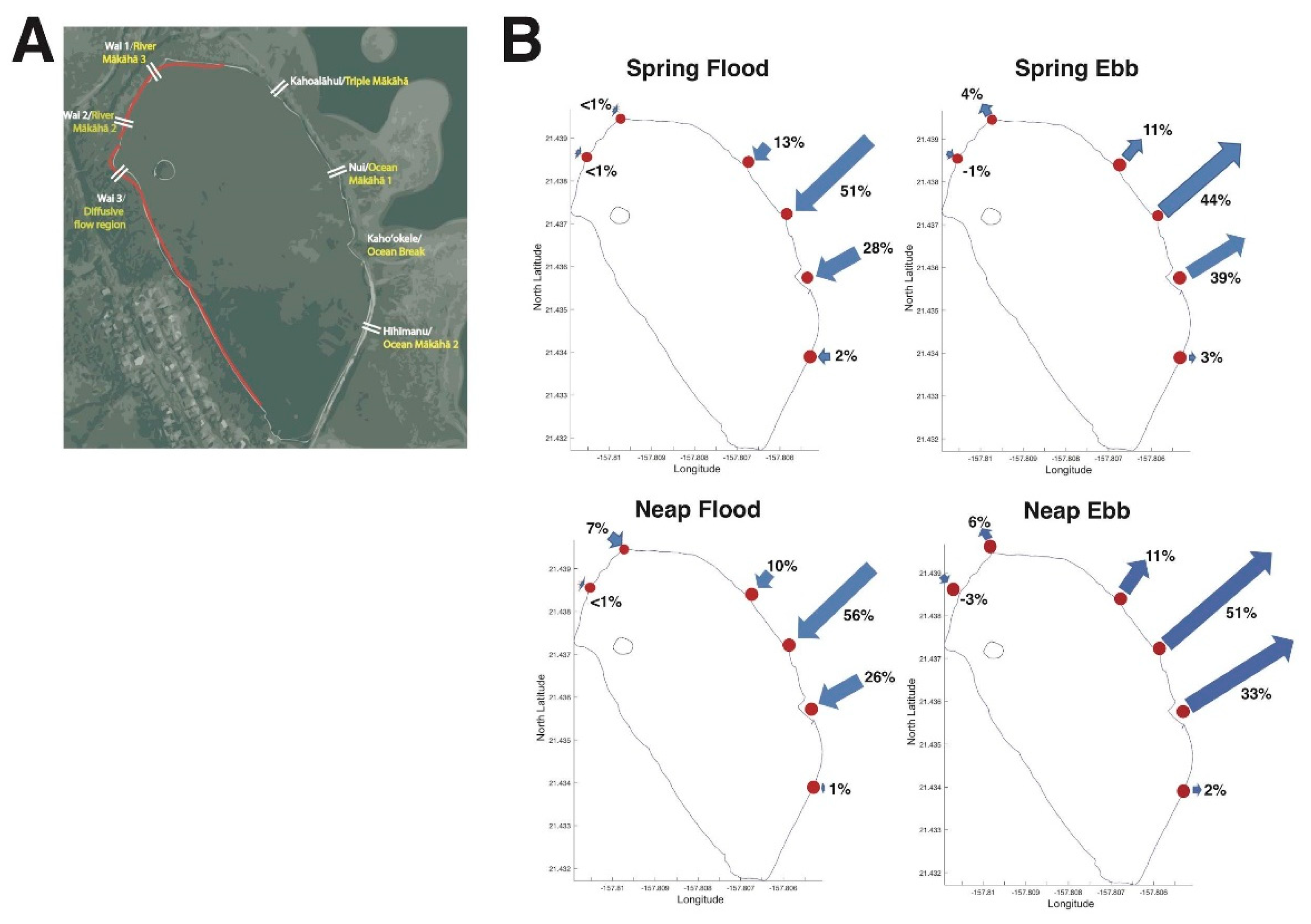
3.1. Restoration from 2014–2018 Shifted Relative Water Volume Flux Contributions of Each mākāhā

3.1.1. Characterizing mākāhā Water Volume Flux Post-Restoration (2018)

Four mākāhā along the eastern kuapā (Hīhīmanu, Kahoʻokele, Nui, Kahoalāhui, Figure 2) were assumed to have bi-directional flow mediated by the semi-diurnal tidal cycle in Kāneʻohe Bay. Three mākāhā in the north and northwest sectors of Heʻeia Fishpond were documented since the early 1900s to provide conduits for surface water inputs into the loko iʻa (Figure 1B). Wai 1 and Wai 2 were restored over the course of this study. Wai 1 is located closest to the mouth of Heʻeia Stream and allows the bidirectional exchange of fresh and oceanic water [30], whereas Wai 2, located 100 m upstream, has a unidirectional flow of surface water into the loko iʻa. The most upstream mākāhā was destroyed during flood events in 1927 and 1965 and has not yet been restored and, measurements with current meters in this area were not possible.

Precipitation and stream discharge were used as criteria to select water volume flux measurements sampling dates with similar meteorological conditions pre- and post-restoration (Table S3). While daily rainfall ranged from 0.05 cm to 1.32 cm in 2012 (pre-restoration) (mean 0.76 ± 0.6 s.d. cm), it ranged slightly higher from 0 cm–2.29 cm (mean 1.23 ± 0.87 s.d. cm) in 2018 (post-restoration). Similarly, Haʻikū Stream discharge ranged from 0.04 m³ s⁻¹–0.07 m³ s⁻¹ (mean 0.06 ± 0.013 s.d. m³ s⁻¹) in 2012 (pre-restoration), and from 0.06 m³ s⁻¹–0.11 m³ s⁻¹ (mean 0.085 ± 0.03 s.d. m³ s⁻¹) in 2018 (post-restoration). Wind direction ranged from E to NE (average wind direction ~50°) with magnitude ranging from 10 to 13 knots pre-restoration and from E to NE (average wind direction ~60°) with magnitudes of 3–13 knots post-restoration.

As each mākāhā was constructed at varying heights from the loko iʻa substratum, flood tide onset and end were defined as low slack water (LSW, water volume flux = 0 m³ s⁻¹) tide stage and high slack water (HSW, water volume flux = 0 m³ s⁻¹), respectively. Conversely, ebb tide onset and end were defined as HSW and LSW, respectively. LSW levels range from 0.2 m at Kahoalāhui to 0.65 m at Kahoʻokele and Wai 1. HSW levels range from ~0.5 m at Kahoalāhui to 1.1 m at Kahoʻokele. The consistently high water level at Wai 1 likely due to continuous baseline stream flow into the loko iʻa. We note that Wai 2 exhibits an atypical rating curve as a wooden board in the mākāhā restricts discharge into the loko iʻa only when water levels are higher than the board (Figure 2, Wai 2).

Mean and peak water volume flux were highest during flood tides at all mākāhā. The fastest mean water volume flux (4.18 m³ s⁻¹ at SF and 2.26 m³ s⁻¹ at NF) and peak water volume flux (9.70 m³ s⁻¹ at SF and 5.41 m³ s⁻¹ at NF) were recorded at mākāhā Nui (

Table 3. Water volume flux (WVF) dynamics in Heʻeia Fishpond post-restoration (2018).

	Mean WVF (m3 s−1)	Peak WVF (m3 s−1)	Tidal Cycle Length (h)	Cum. Flux per Tidal Cycle (m3)	WVF Rate (m3 h−1)	Volume Exchanged per Tidal Cycle (m3)	Relative WVF
Spring Flood				191660	31778	191660	100.00%
Wai 2	0.05	0.16	4.43	840	190	840	0.44%
Wai1	0.40	0.93	4.55	7140	1569	7140	3.37%
Kahoalāhui	1.47	2.76	4.36	24420	5601	24420	12.74%
Nui	4.18	9.70	6.29	97800	15548	97800	51.03%
Kahoʻokele	2.02	4.69	7.29	54380	7460	54380	28.37%
Hīhīmanu	0.39	0.95	5.02	7080	1410	7080	3.69%
Spring Ebb				−174880	−30851	−174880	100.00%
Wai 2	0.07	−0.09	5.50	1560	284	1560	−0.89%
Wai1	−0.32	−0.63	6.32	−7600	−1203	−7600	4.35%
Kahoalāhui	−0.87	−1.86	6.31	−20220	−3204	−20220	11.56%
Nui	−3.60	−4.86	5.53	−76320	−13801	−76320	43.64%
Kahoʻokele	−1.10	−3.12	5.50	−67520	−12276	−67520	38.61%
Hīhīmanu	−0.17	−0.43	7.35	−4780	−650	−4780	2.73%
Neap Flood				141384	16717	141384	100.00%
Wai 2	0.05	0.20	7.41	1300	175	1300	0.92%
Wai1	0.32	0.98	8.29	9720	1172	9720	6.87%
Kahoalāhui	0.51	1.08	7.31	13620	1863	13620	9.63%
Nui	2.26	5.41	9.46	78744	8324	78744	55.70%
Kahoʻokele	1.35	2.52	7.30	36440	4992	36440	25.77%
Hīhīmanu	0.05	0.24	8.20	1560	190	1560	1.10%
Neap Ebb				−159938	−10584	−159938	100.00%
Wai 2	0.88	−0.09	17.46	5640	323	5640	−3.53%
Wai1	−0.17	−0.57	15.50	−9880	−637	−9880	6.18%
Kahoalāhui	−0.30	−0.9	15.50	−17100	−1103	−17100	10.69%
Nui	−1.60	−3.19	14.09	−81298	−5770	−81298	50.83%
Kahoʻokele	−0.86	−1.80	17.10	−53280	−3116	−53280	33.31%
Hīhīmanu	−0.08	−0.25	14.34	−4020	−280	−4020	2.51%

). In addition, flood tidal cycle duration was shorter than ebb at all mākāhā at both Spring and Neap, mean tidal duration was 5.23 ± 1.20 s.d. h and 8.00 ± 0.84 s.d. h for SF and NF, respectively, whereas mean tidal duration was 6.09 ± 0.73 s.d. h and 15.67 ± 1.38 s.d. h for SE and NE, respectively. Taken together, the shorter lag time at high water vs. low water, longer-duration dropping tides and stronger flood than ebb currents suggest that Heʻeia Fishpond is a flood-dominant system.

3.1.2. Changes in Relative Water Volume Flux Post-Restoration

We evaluated the relative contribution of each mākāhā to loko iʻa water exchange during SF, SE, NF, and NE in order to gain insight into how restoration altered circulation in Heʻeia Fishpond. Prior to restoration, Ocean Break, the 0.9 m elbow wall bridging the 56 m gap in the eastern kuapā was lower than the adjoining sections of wall, restricting water exchange to high tidal stages, when the water level exceeded the height of Ocean Break. Restoration resulted in a significant shift in water exchange in the seaward kuapā. The spatial pattern of flushing in Heʻeia Fishpond remains dominated by the mākāhā in the northeast quadrant of the loko iʻa for all tidal stages. Nui, Kahoʻokele, and Kahoalāhui together account for 92% of the water exchanged at spring flood, 94% at spring ebb, 91% at neap flood and 95% at neap ebb tide whereas the southern and eastern edges of the loko iʻa experience relatively low flushing.

When comparing site–specific water volume flux rates pre-restoration (2012) to post-restoration (2018), it becomes evident that the relative magnitude of water volume flux specific to each mākāhā changed due to restoration practices: The total amount of water volume exchanged in a complete tidal cycle decreased from 241,413 m³ pre-restoration to 194,700 m³ post-restoration for flood tide and decreased from −241,685 m³ pre-restoration to −173,080 m³ post-restoration for ebb tide (

Table 4. Change in water volume flux (WVF) rates through mākāhā pre-restoration (2012) and post-restoration (2018).

Mākāhā	Flood Tide				Ebb Tide
	Pre-Restoration		Post-Restoration		Pre-Restoration		Post-Restoration
	Volume Exchange per Tidal Cycle (m3)	Relative WVF	Volume Exchange per Tidal Cycle (m3)	Relative WVF	Volume Exchange per Tidal Cycle (m3)	Relative WVF	Volume Exchanged per Tidal Cycle (m3)	Relative WVF
Wai 2	2057	0.85%	1300	0.67%	−5515	2.28%	5640	−3.25%
Wai 1	2249	0.93%	9720	5.10%	−5791	2.40%	−9880	5.70%
Kahoalāhui	4106	1.71%	24420	12.54%	−5802	2.41%	−20220	11.68%
Nui	31101	12.88%	97800	50.24%	−26886	11.12%	−76320	44.10%
Kahoʻokele/OB	197820	81.94%	54380	27.93%	−192780	79.76%	−67520	39.01%
Hīhīmanu	4081	1.69%	7080	3.61%	−4912	2.03%	−4780	2.76%
Mākāhā Total	241,413	100.00%	194,700	100.00%	−241,685	100.00%	−173,080	100.00%

). Pre-restoration, Ocean Break facilitated the largest amount of volume exchange contributing approximately ~80% to total water exchange at both flood and ebb tidal cycles (81.94% for flood, 79.76% for ebb) with mean water velocities of 11.53 m³ s⁻¹ and −13.55 m³ s⁻¹ [42]. Pre-restoration, Nui contributed the second largest amount of volume exchange with 12.88% for flood and 11.12% for ebb tide and mean velocities of 1.75 m³ s⁻¹ and −0.5 m³ s⁻¹ [42]. While contributing only 10% to water exchange pre-restoration, post-restoration Nui is presently the site with largest water volume exchange. Post-restoration, Nui facilitated about half of the volume exchanged (50.24% at flood tide, 44.1% at ebb tide, Figure 3) with much higher mean water volume flux of 4.18 m³ s⁻¹ and −3.6 m³ s⁻¹ (Table 4) than pre-restoration. In contrast to pre-restoration, Kahoʻokele now accounts for the second largest volume exchanged (27.93% and 39.01% for flood and ebb tide respectively, Figure 3) with lower mean water volume flux of 2.02 m³ s⁻¹ and −1.1 m³ s⁻¹ compared to pre-restoration. Kahoalāhui is composed of three individual mākāhā post-restoration and together they account for the third largest water volume—roughly 10% of contribution to total water volume flux. The relative contribution in the magnitude of Kahoalāhui increased about six-fold for flood tide and five-fold for ebb tide from pre-restoration to post-restoration (from 1.71% to 12.54% for flood tide and 2.41% to 11.68% for the ebb tide, Table 4). Hīhīmanu did not experience significant changes due to restoration: While accounting for 1.69% at flood and 2.03% for ebb pre-restoration, it now accounts for 3.61% and 2.76% at flood and ebb, respectively (Table 4). Mean water volume flux ranged from −0.12 m³ s⁻¹ to 0.28 m³ s⁻¹ pre-restoration and is now −0.17 m³ s⁻¹ to 0.39 m³ s⁻¹.

In terms of overall volume exchange, the river mākāhā continue to play minor roles in water exchange. In 2018, water volume flux rates measured at Wai 1 were similar to pre-restoration with a relative water volume flux magnitude of 3–7% and low mean flow rates (Figure 3, Table 4). Water passing through Wai 1 increased from 0.93% pre-restoration to 5.1% post-restoration for flood tide, and 2.4% pre-restoration to 5.7% post-restoration for ebb tide. Water volume flux increased from 0.09 m³ s⁻¹ and 0.1 m³ s⁻¹ pre-restoration to 0.4 m³ s⁻¹ and 0.32 m³ s⁻¹ post-restoration. Pre-restoration Wai 2 accounted for 0.85% of water exchange during flood tide and accounts for a slightly decreased water exchange of 0.67% post-restoration for flood tide. For ebb tide, the water exchange reversed from 2.28% pre-restoration to –3.25% post-restoration. Wai 2 displayed unidirectional flow into the loko iʻa, regardless of tidal state with solely positive flow velocities and accounting for the lowest water volume flux measured.

3.2. Decrease in loko iʻa Volume and Residence Time Post-Restoration

The majority of the loko iʻa has relatively uniform and shallow bathymetry of ~0.9 m with the deeper portions around the mangrove island and Ocean Break [26]. Prior to restoration, water exchange along the eastern kuapā only occurred when the water depth exceeded the height of the elbow wall at Ocean Break. Pre-restoration, ~90% of loko iʻa water exchange occurred in the northeast corner of the loko iʻa via Ocean Break (~80%) and Nui (~10%), suggesting that the eastern half of the loko iʻa was better mixed and less stratified than the western side [30,34]. Water volume exchange before restoration was also found to be largely tidally driven, with the greatest volume exchange at mid-tide: ~77% during spring tide and ~42% during neap tide.

Given changes in water volume flux in Heʻeia Fishpond due to restoration, we determined post-restoration loko iʻa volume and residence time for SF, SE, NF, NE. Heʻeia Fishpond is deepest during SF tide (Figure 4A), averaging 0.89 ± 0.12 m with a minimum water depth of 0.63 m in the center of the loko iʻa and a maximum water depth of 1.46 m around the mangrove island in the northwestern corner of the loko iʻa. During SF, the maximal volume of the loko iʻa is 264,730 m³ (Figure 4B). The minimum water volume occurs during SE tide when the loko iʻa is 48,060 m³ or 20% of the SF volume (Figure 4B). The mean loko iʻa depth at spring ebb tide is 0.17 m ± 0.12 m and ranges from 0 m in the center to 0.74 m around the mangrove island in the northwestern corner of the loko iʻa. The NF tidal volume is 149,550 m³, 56% of the SF tidal volume, with a mean depth of 0.50 m ± 0.12, ranging from 0.25–1.08 m. NE depth ranges from 0–0.79 m, averaging 0.22 ± 0.12 m. NE tidal volume is 63,160 m³. Restoration regimes resulted in a considerable change of loko iʻa volume from pre- (2007) to post-restoration (2018): SE tide loko iʻa volume decreased 16,010 m³, SF volume decreased 17,990 m³, NE volume decreased 14,890 m³ and NF volume increased 15,660 m³ (Figure 4B). Thus, as a result of removing the elbow wall and installing a sixth mākāhā (Kahoʻokele), Heʻeia Fishpond is shallower and has a lower volume at all tidal states except NF.

We calculated that post-restoration, approximately 82% of the loko iʻa water is exchanged during the ebb–flood transition at spring tide. During the neap tide ebb-flood transition, 58% of the loko iʻa water is exchanged. To be consistent with previous work by Young [30], we defined one flushing cycle as the time that it takes to flush out 82% of loko iʻa water during spring ebb tide and to replenish that water again with new Kāneʻohe Bay water during spring flood tide or 12 h Based on the assumption that the incoming water would mix uniformly with the water remaining in the loko iʻa during the first flushing cycle (18%), about 3 flushing cycles are required to mix the initial 18% of water to a <1% dilution. Therefore, the post-restoration minimum residence time of Heʻeia Fishpond is ~ 32 h or under 3 flushing cycles, and occurs during spring tide when water exchange is maximal. In contrast, when water exchange is minimal (e.g., neap tides), the maximum residence time is 64 h More than 5 flushing cycles or 64 h are required to mix the 42% of water retained down to <1% dilution. Water exchange during ebb flood transition experienced a 4.51% increase (from 77.34% pre-restoration to 81.85% post-restoration, Table 4) at spring tide. During neap tide water exchange increased 16.06% (from 41.71% pre-restoration to 57.77% post-restoration, Table 4). As a result, minimum water residence time decreased from 38 h at spring tide pre-restoration to 32 h (~1.5 days) at spring tide post-restoration and maximal residence time during neap tides decreased from 102 h (~8.5 days) at spring tide pre-restoration to 64 h (~5.5 days) at spring tide post-restoration.

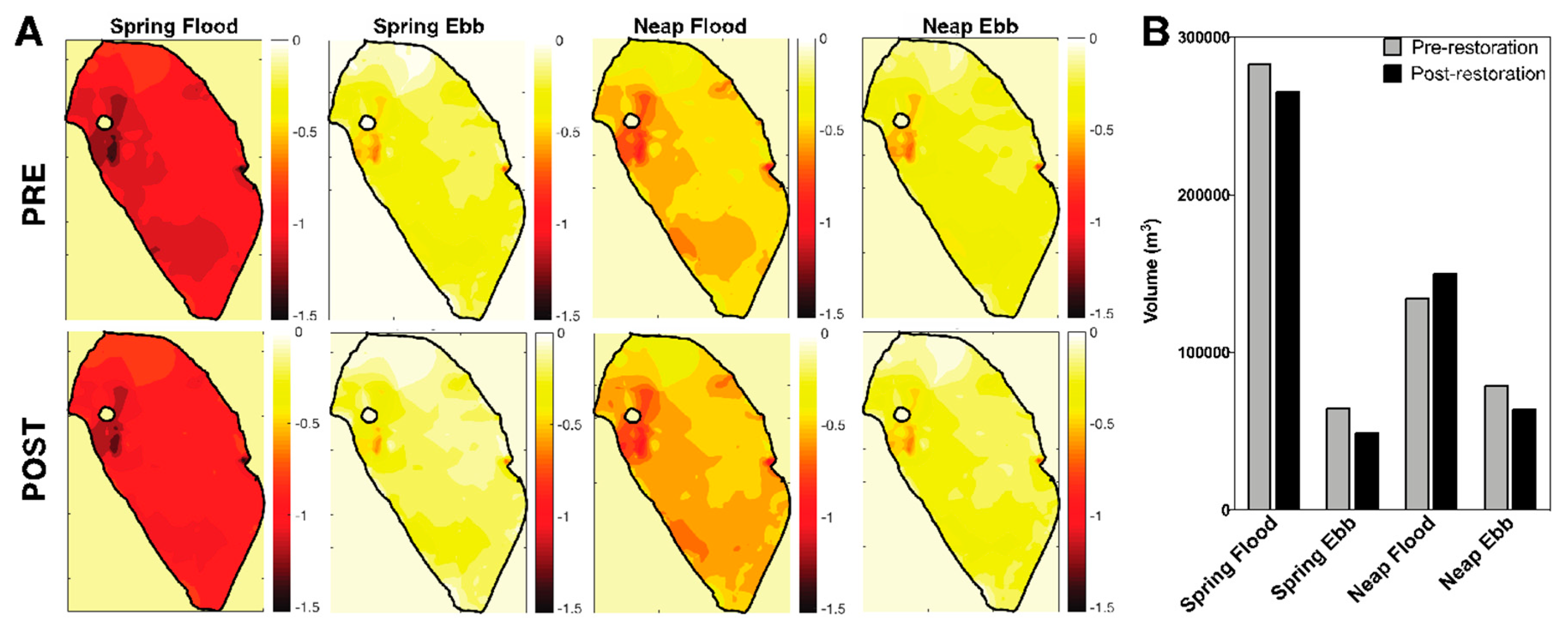
3.3. Spatial Salinity Distribution Significantly Altered due to Restoration

The water column geochemistry of Heʻeia Fishpond is influenced by the mixing of distinct water masses: surface water from Heʻeia Stream, whose discharge depends on precipitation; submarine groundwater discharge, composed of a mixture of fresh water from an underground aquifer and recirculated seawater [43]; and seawater from Kāneʻohe Bay that fluctuates with tidal pumping. Built at the interface of Heʻeia Stream and Kāneʻohe Bay, Heʻeia Fishpond exhibits a typical vertical salinity gradient—a less dense, freshwater lens atop a more dense, saltier water mass—although mixing of these water masses does occur with increased river flow, winds, and tides. A major motivation for the biocultural restoration of Heʻeia Fishpond was to increase the freshwater influence in the loko iʻa. Kiaʻi loko hypothesized that brackish conditions would drive primary production of diatoms—a major food source for juvenile mullet, which is a target species. Surface and bottom salinities were measured using a handheld YSI at several locations in Heʻeia Fishpond (Figure 5A). We selected two pre-restoration sampling events from 2014 and three post-restoration sampling events from 2017 with similar meteorological conditions (Tables S4 and S5). Salinity measurements from pre- and post-restoration work was analyzed as an indicator of loko iʻa circulation, mixing, and stratification.

Surface salinity distribution pre- and post-restoration display a strong spatial gradient (Figure 5B, left panels). The highest salinities in both cases were measured along the ocean-ward kuapā near Nui and the Ocean Break/Kahoʻokele (station P10), while the lowest salinity was measured along Heʻeia Stream near Wai 2 (station P3, L07). However, mean pre-restoration salinity was significantly higher than post-restoration salinity, 27.4 ± 4.86 ppt and 20.5 ± 10.41 ppt, respectively (p-value < 0.01). With similar meteorological conditions, these data indicate a weaker freshwater influence and stronger salinity gradient pre-restoration. Before restoration, the freshwater wedge did not extend past the western edge of the mangrove island, where salinities ranged from 20–25 ppt (stations P2, P4, P5) and further west, salinities rose to 25–30 ppt (stations P1, P6, P7, P8, P9). Post-restoration however, salinity ranged from 0.10–32.59 ppt with the freshwater wedge from the river extended beyond the mangrove island, which ranged from 15–20 ppt (stations L06, L08, L09), with salinities further west rising to above 20 ppt (station L01 and L05) and 25–30 ppt (stations L02, L03, L04, L11, M03). The presence of strong spatial gradient throughout the restoration process suggests that freshwater from Heʻeia Stream is more prevalent along the northwestern side of the loko iʻa, whereas tidal pumping from Kāneʻohe Bay dominates the southeastern side of the loko iʻa.

As expected, bottom waters of the loko iʻa had a higher salinity than the surface, however, post-restoration salinity exhibited limited gradient structure post-restoration, whereas the loko iʻa bottom pre-restoration was entirely homogeneously mixed with no detectable freshwater influence (Figure 5B, right panels). Mean bottom salinities were significantly higher pre-restoration (31.99 ± 1.82 ppt) as compared to post-restoration (25.17 ± 8.12 ppt), p-value < 0.1. Post-restoration, the influence of freshwater from Heʻeia Stream became more evident, with the majority of the loko iʻa salinity ranging from 20–25 ppt (Figure 5B, lower right panel). Similar to the surface salinity spatial distribution, highest measurements were taken near the Kahoʻokele and Nui and the lowest measured bottom salinities were taken at Wai 2.

3.4. Restoration-Driven Changes to Circulation Altered Microbial Biomarker Spatial Distribution

To understand the consequences of Paepae o Heʻeia’s restoration regime on biological–physical interactions in the loko iʻa, we quantified the abundance of microbial biomarkers that have been used previously to track fecal contamination within bodies of water. We focused on 3 specific bacterial groups: Enterococcus and Bacteroidales, indicators of contamination from mammals and C. marimammalium, an indicator for contamination from avian sources, to investigate how increasing freshwater inputs into the loko iʻa potentially affect the biogeography of pathogens.

Discrete samples were collected from a network of stations across the loko iʻa along a transect from Wai 2 to Kahoʻokele to capture the salinity gradient observed previously (Figure 5A, L03, L06, L07, L09, L10). In addition, we sampled at a higher resolution around the mangrove island on the interior of the loko iʻa in order to consider the influence of the large B. ibis rookery housed in the R. mangle stand. Contrary to expectations, amplification of the 16S rDNA genes from the family Bacteroidales (GenBac3) and the genus Enterococcus (Entero 1a) from samples pre- and post-restoration showed no significant difference when averaged across all stations (Figure 6A). We hypothesized that grouping together data may have masked changes in biomarker spatial distribution that occurred due to restoration. We mapped the mean concentration (16S copies 100 mL⁻¹) onto the stations and used a rectangular grid with ~1 m spacing to determine whether the biogeography of Enterococcus and Bacteroidales changed from 2014 to 2017 (Figure 6B,C respectively). We found that prior to restoration, the mean concentration of Bacteroidales was higher than 10⁴ copies per 100 mL across the entire western side of the loko iʻa. In contrast, post-restoration, Bacteroidales concentrations higher than 10⁴ copies per 100 mL were restricted to a geographically smaller area of the loko iʻa, adjacent to Wai 2 and the diffuse flow region and lower in the center of the loko iʻa (Fig 6B and 6C, top row). Indeed, when grouped by salinity, freshwater stations showed a statistically significant decrease in Bacteroidales concentration post-restoration (Figure 6D, top row, white). General additive mixed model (GAMM) analysis confirmed that concentration of Bacteroidales negatively correlates with salinity (Figure 6E, top row,

Table 5. Summary of general additive mixed model (GAMM) analysis. Summary output from the general additive mixed model analyis in R. Input Formula: LogConcentration ~ (1 | Date) + Pre- vs. –postrepair + Salinity; ¹ Significance codes: 0 ‘***’ 0.001 ‘**’ 0.01 ‘*’ 0.05.

Bacterial Indicator		Estimate	Std. Error	df		t Value	Pr (>|t|)	Signif. Codes 1
C. marimammalium	Intercept	4.99266	0.37574	9.16611	13.287		2.69 × 10−7	***
	Pre-vs. post repair	0.96856	0.4402	4.42676	2.2		0.086085
	Salinity	−0.04652	0.01226	57.66017	−3.794		0.000357	***
Bacteroidales	Intercept	6.36231	0.48919	10.03302	13.006		1.32 × 10−7	***
	Pre-vs. post repair	0.45987	0.56039	4.46269	0.821		0.453
	Salinity	−0.09205	0.01671	57.73214	−5.509		8.75 × 10−7	***
Enterococcus	Intercept	5.14077	0.36391	12.62958	14.127		4.12 × 10−9	***
	Pre-vs. post repair	0.45003	0.39462	4.63367	1.14		0.31
	Salinity	−0.0794	0.01361	57.97529	−5.823		2.66 × 10−7	***

), with the highest concentrations found at stations with the lowest salinity.

We also found that when values were grouped across all stations Enterococcus concentrations did not change significantly over the course of restoration (Figure 6A, middle row). However, unlike Bacteroidales, the spatial distribution of Enterococcus pre- and post-restoration was structured with highest concentrations along the western edge of the loko iʻa (10⁴ copies per 100 mL) and decreasing concentrations proceeding eastward down to 10²–10³ copies per 100 mL (Figure 6B,C, middle row). The lack of difference in pre- vs. post-restoration data was also supported by binning the stations along a salinity gradient (Figure 6D, middle row). As expected, the general additive mixed model (Figure 6E, middle row) confirmed that Enterococcus has increased abundance in low salinity environments (Table 5).

To assess B. ibis fecal contamination, we first developed microbial source tracking tools by adapting primers specific to the 16S rDNA gene of C. marimammalium (Table 2, GFCf and GFCr). These primer pairs had previously been used to detect fecal contamination from gulls, geese, ducks, and chickens [41]. GFC primers specifically amplified fecal DNA from B. ibis living at Heʻeia Fishpond (Figure S1) and were used to determine the extent of contamination from B. ibis fecal sources in the loko iʻa. Pre-restoration, B. ibis fecal contamination was significantly higher across all stations (mean concentrations of 2–4 × 10⁵ copies 100 mL⁻¹) as compared to 10⁴ copies 100 mL⁻¹ post-restoration (Figure 6A, bottom row), p < 0.01. Pre-restoration concentrations of B. ibis fecal indicator bacteria were higher across all stations than both Bacteroidales and Enterococcus (Figure 6B), with greater than 10³ copies per 100 mL detected at the oceanic stations. In contrast, post-restoration concentrations of C. marimammalium decreased by 2 orders of magnitude, and these differences were statistically significant at the fresh and brackish stations (Figure 6D, bottom row). General additive mixed model (GAMM) analysis indicates that while the negative correlation between B. ibis fecal indicator bacteria and salinity is not as strong as with Bacteroidales and Enterococcus, it does exist (Table 5).

We note two interesting differences in microbial indicator concentrations and biogeography post-restoration. First, we note the appearance of a region where microbial indicator concentrations are low (Figure 6C). We note that differences in the station locations pre- vs. post-restoration may have altered the interpolation of biomarker concentrations. Alternatively, this may suggest that post-restoration, circulation patterns in the center of the loko iʻa have resulted in a well-flushed zone. Secondly, spatial variation in 16S copy concentration for all three molecular markers was greater pre-restoration compared to post-restoration (Figure 6D). The variation coefficient (standard deviation divided by mean) pre-restoration was 0.31 (C. marimammalium), 0.43 (Enterococcus), 0.4 (Bacteroidales), while the variation coefficient post restoration was 0.16 (C. marimammalium), 0.32 (Enterococcus), 0.31 (Bacteroidales). We interpret this difference as an indication that pre-restoration, the loko iʻa was less homogeneously mixed than post-restoration.

4. Discussion

Embedded between land and sea, Heʻeia Fishpond is a powerful natural laboratory. We have been provided the unique opportunity to examine how historical land use change has altered the functions of coastal habitats and how biocultural restoration maintains and improves the integrity of these coastal ocean ecosystems in the face of rapid global change. In the current study, we utilized a comprehensive time series dataset of in situ deployments, discrete sampling, and empirical observations to draw a link between restoration efforts and changing loko iʻa circulation, as well as water quality dynamics. Specifically, we examined the impact of invasive mangrove removal around the northern loko iʻa periphery from 2014–2017 and Pani ka Puka, repair of the Ocean Break in 2015, presenting a comparison of pre- vs. post-restoration ecosystem dynamics along multiple parameters.

4.1. Hoʻoniho ka niho (Interlock the Stones [44]): Water Volume Flux Changes due to Kuapā Repair

Generally, understanding the physical environment of Heʻeia Fishpond advances our knowledge of the dynamic biochemical and physical interactions in Hawaiian estuarine ecosystems. In repairing the physical infrastructure of Heʻeia Fishpond, Paepae o Heʻeia has set the stage for the ecology of the loko iʻa to return to the original conditions engineered by kūpuna (elders, ancestors) of Heʻeia: a brackish body of water with a consistent volume, maintained by regulated mixing of fresh and marine inputs to facilitate phytoplankton growth. Our study confirms that during baseline conditions, coastal loko iʻa circulation patterns are driven by a combination of either tidal pumping or stream velocity, depending on the location of the mākāhā [30,45]. Water volume flux rates during SF and SE tides from mākāhā bordering Kāneʻohe Bay (Hīhīmanu, Kahoʻokele, Nui, Kahoalāhui), suggest that the loko iʻa is more influenced by oceanic inputs (>95% total mean water volume flux) than freshwater inputs (<5% total mean water volume flux) from Heʻeia Stream during baseline conditions at both pre- and post-restoration (Table 3 and Table 4, Figure 3).

Prior to Pani ka Puka, Heʻeia Fishpond acted largely as an unconfined system during spring tides, when the spring flood tide exceeded the height of Ocean Break. In essence, because the Ocean Break was lower in height than the surrounded kuapā, the entire 56 m wide section of Ocean Break functioned like a mākāhā when tidal pumping in Kāneʻohe Bay was higher than the provision elbow wall. Pre-restoration, we observed enormous water volume flux at spring tides, ~80% exchange almost exclusively from Ocean Break (Table 4). However, during neap tides, the loko iʻa was more confined with less exchange and circulation in the southeastern portion of the loko iʻa. In 2015, this expansive section of the wall was repaired and Kahoʻokele was built, shifting relative mākāhā exchange rates at Kahoʻokele to ~30% post-restoration. This dynamic is also reflected in mean water volume flux rates: Pre-restoration, Ocean Break had the highest mean water volume flux rates of ~12–14 m³ s⁻¹ (Table 4), while the Kahoʻokele water volume flux rates post-restoration are dramatically lower (now ~ 1 m³ s⁻¹, Table 3 and Table 4). Mean water volume flux rates at other mākāhā generally increased from pre-restoration to post-restoration, an indication that nearby mākāhā somewhat compensate for the difference in water volume flux between Ocean Break and Kahoʻokele. However, the general “C” shape of rating curves remained similar (Figure 3). In its current state, the addition of Kahoʻokele renders Heʻeia Fishpond a confined system at all tidal states with adequate water exchange in the southeastern region. These findings are supported by Ertekin et al. [46] who modeled circulation patterns at two different Aliʻi loko iʻa on Molokaʻi, which concluded that the number of mākāhā plays a significant role in improving tidal circulation. They concluded that mākāhā distance and location in relation to the physical forces at work (tidal activity, wind, loko iʻa bathymetry, stream location) affected circulation inside the loko iʻa.

Our results suggest that oceanic mākāhā water volume flux is also dependent upon wind forcing, in particular for mākāhā aligned with the trade winds (~70°). Nui and Kahoʻokele account for ~50% and ~30% of total water volume flux respectively, Figure 3. These mākāhā also have the largest cross-sectional areas (Nui: 6.48 m; Kahoʻokele: 3.05 m, Table 1), and are positioned most in–line with the predominant trade wind direction, Nui has a bearing of 63° and Kahoʻokele has a bearing of 80° (Table 1). Wind blowing from the northeast across Kāneʻohe Bay, can accelerate (if the wind aids) or dampen (if the wind opposes) water flow through Nui and somewhat Kahoʻokele, which is aligned with the predominant wind direction of 70°. We also noted that the channel floor of Kahoʻokele is deeper than the adjacent benthos of both the loko iʻa interior and Kāneʻohe Bay. Thus, the mākāhā floor depth may allow slightly higher water volume flux through Kahoʻokele due to lower resistance to water volume flux. In contrast, Kahoalāhui and Hīhīmanu have considerably smaller relative water volume flux (together accounting for ~15%, Figure 3) as the individual channels of Kahoalāhui have small cross–sectional areas and Hīhīmanu has the smallest cross–sectional area (2 m, Table 1), in addition to being positioned at 48° and 111°, respectively. The notion that wind can influence the rate of water flow through mākāhā is supported by a study by Yang [47] who suggested that the rate of water flow through the mākāhā may be altered by wind accelerating or dampening flow when the body of water was large enough. Kāneʻohe Bay and Heʻeia Fishpond are both large enough, and shallow enough to be affected by wind stress in such a way as to act as a secondary driver of water volume flux in this system.

We found that the river mākāhā have significantly lower relative water volume flux rates during base flow conditions (i.e., non-storm) pre- and post-restoration (Wai 1 and Wai 2 together ~5%). Water volume flux through Wai 1, the most seaward mākāhā along the Heʻeia Stream, is dependent on tidal activity due to its proximity to Kāneʻohe Bay, making it the only freshwater mākāhā that allows bi-directional water flow. Under baseline conditions, the relative water volume flux of water passing through Wai 1 during flood tide is balanced by the amount of water that flows out during ebb tide (Table 3). At flood tides, flow out of Wai 1 is dampened by Heʻeia Stream, due to flow in the opposite direction into the loko iʻa, while Heʻeia Stream flow is additive during ebb tides. Due to a dam-like structure in the mākāhā (Figure 2), Wai 2 has little to no detectable tidal signal and exhibits exclusive unidirectional flow from Heʻeia Stream into the loko iʻa that is largely dependent stream discharge and precipitation in the Heʻeia watershed [30,45,47]. During episodic storm events, strong freshwater water volume influx can have pronounced effects on the loko iʻa system [30], yet our water volume flux measurements were all conducted at baseline/low flow conditions. We anticipate that the relative contribution of river mākāhā vs. ocean mākāhā, as well as the balance between ebb vs. flood exchange, is likely to change if Heʻeia Stream discharge increases during storm events. Research comparing baseline to storm conditions to quantify how higher stream velocities affect loko iʻa flushing is currently underway and will be the subject of a subsequent contribution.

Assuming the Heʻeia Fishpond water balance is in steady state, the water volume influx rates should be equivalent to water volume outflux rates. However, we found the difference between spring and neap tidal cycle flow, the sum of flow (m³) for all mākāhā, to be –16,760 m³ or ~8% of total flow between SF and SE tide and 18,554 m³ or ~13% of total flow between NF and NE (Table 4). Post-restoration, this imbalance is most evident in 2 mākāhā: Kahoʻokele, which accounts for 28% of water volume influx, and 39% of water volume outflux during spring tide, and Nui, which accounts for 40% of water volume influx and 44% of water volume outflux during spring tide. This pattern is evident at both spring and neap tidal cycles. We posit that trade winds accelerate flow into the loko iʻa at Nui during flood tide, which as previously discussed is aligned with the prevailing wind direction during sampling (63°, Table 1). However, during ebb tide, the wind force opposes outflow at Nui, and a small proportion of water volume flux is redistributed to other mākāhā channels thereby compensating for the reduced outflow at Nui (Table 3, Figure 4). However, these site–specific differences do not account for all the discrepancy observed pre- and post-restoration. We attribute discrepancies in water volume flux balances to a number of factors. First, the influence of submarine groundwater discharge (SGD) into Heʻeia Fishpond is not accounted for in this study. Previous work quantifying SGD at Heʻeia Fishpond using radon isotope measurements found that the amount of water volume flux from SGD was equal to that of Heʻeia Stream discharge [43,48]. Second, the water volume flux in the diffuse flow region (Figure 1B), as well as gains or losses of water through small holes in the kuapā, was not quantified and has not been accounted for in our water budget. In addition, though every effort was made to choose tidal cycles similar in length and amplitude for rating curves, rating curves were calculated using in situ data from sequential rather than simultaneous deployments due to the limitation of instruments (Table S1). Some degree of variability in tidal length and amplitude among sites likely exists. Finally, the mixed semidiurnal tides cause large variations in tidal length (Table 3), giving rise to some uncertainty in the final water volume flux rates calculated.

4.2. Paepae ke alo (Raise the Face of the Wall [44]): Volume, Residence Time, and Salinity

Pani ka Puka affected loko iʻa volumes and residence times considerably (Figure 4). The addition of a sixth mākāhā (Kahoʻokele) led to increased and faster water volume outflux during both NE and SE tides, corresponding to lower volumes post-restoration. Conversely, whereas no water exchange occurred at Ocean Break during neap tides prior to restoration, Kahoʻokele allows more water volume influx during NF tide compared to before, resulting in a larger loko iʻa volume post-restoration during this tidal stage (Figure 4). These increased water masses cannot be compensated entirely with the flow (1–2 m³ s⁻¹) through Kahoʻokele, which has a smaller cross–diameter, 3.05 m as compared to Ocean Break, 56 m (Figure 1C,D). We predicted that restoration would result in shorter residence times, particularly during neap tides. Indeed, total exchange rates during spring tides were 5% higher post-restoration, with a 12% shorter minimum residence time of 32 h as compared to 38 h pre-restoration. Changes in post-restoration circulation are more marked during neap tides – water exchange has increased 16% and maximum residence time has decreased 37% from 102 h to 64 h These residence time calculations are tempered by the following assumptions: (1) uniform mixing of the loko iʻa water column, (2) all flood and ebb tides are 6 h, (3) mākāhā are the only source of water exchange. However, salinity measurements at the surface and benthos indicate that the water column is sometimes mildly stratified. Furthermore, our data show a large range in tidal cycle duration variability, ranging from 4.43–17.46 h (Table 3). Lastly, submarine groundater discharge and input from the diffuse flow region (Figure 1B) likely are other indirect sources of water exchange. The difference in minimum and maximum residence times emphasizes the importance of differentiating between tidal states when looking at the effects of restoration on the physical environment of the loko iʻa.

Concomitant mangrove removal around the stream mouth corresponded with an increase in water volume flowing through Wai 1 from ~1–2% pre-restoration to ~5% post-restoration (Figure 1E and Table 4) and a freshening of the loko iʻa post-restoration. At the end of the period of this study, Wai 2 was not fully clear of R. mangle and also showed little change in discharge between pre- and post-restoration. We conclude that mangrove removal positively correlates with increased water flow and subsequently improved loko iʻa circulation. Increased freshwater volume flux is also reflected in the salinity distribution, which shows a much stronger freshwater signal around the river mākāhā in post-restoration compared to pre-restoration (Figure 5B). We expect that continued removal of mangrove along the loko iʻa periphery would increase stream velocity and the mass of freshwater entering Heʻeia Fishpond. It is also evident that mixing from the ocean is more limited post-restoration, and thus the freshwater coming in may have a greater overall effect on the salinity. Moreover, the temperature of the surface water is often much lower than marine inputs and given concerns about fish stress linked to sea surface warming trends [29], mixing of cooler water may be beneficial to fish survival. In addition, increased freshwater and nutrient input may be beneficial for native macroalgae and phytoplankton to thrive, which is the primary food source for the herbivorous target fish species. While we can only speculate as to the historical biogeochemistry of Heʻeia Fishpond, the abundance of evidence suggests that increasing freshwater input is necessary for proper management of native marine species. As this is the first study we are aware of that reveals a correlation between mangrove removal and improved loko iʻa circulation, we recommend long–term monitoring of fish and phytoplankton diversity and biomass, particularly near the stream so that the connection between mangrove removal, stream flow, and nearshore fishery health can be fully understood.

4.3. Pani hakahaka (Close Gaps/Vacancies [44]): Microbial Indicators as Markers of Watershed Connectivity

To assess water quality and associated human health risk, we used two broad–spectrum microbial bioindicators used by the US Environmental Protection Agency [49,50]. We used primers that targeted the Bacteroidales family (GenBac3) and the Enterococcus genus (Entero1a), bacteria that are common in the feces of mammals (Table 2). These non–pathogenic microbes are easy to quantify and have decay rates similar to those of the pathogens of interest [51], hence, they can be strongly associated with the presence of pathogenic microorganisms derived from upstream in the watershed. By performing co-registered sampling of salinity and microbes, we were able to directly correlate fecal indicator concentrations with salinity, an abiotic factor that strongly influences abundance [49,52,53]. We hypothesized that shorter residence time and increased water volume flux would lower the concentration of Bacteroidales and Enterococcus in Heʻeia Fishpond. Instead, we found no significant overall difference in surface mammalian fecal indicator bacteria before and after restoration (Figure 6A). We found coherence between spatial distribution of mammalian fecal indicators with surface salinity (Figure 6B): post-restoration, lower salinity (e.g., more fresh water) in the northwestern sector of the loko iʻa corresponded with even higher concentrations of bacterial indicators as compared to pre-restoration whereas higher salinity in the oceanic–dominated areas of the fishpond had even less fecal contamination than pre-restoration. From the spatiatl distrution of each marker (Figure 6D), we attribute the increase in mammalian fecal bacteria in the northwest area of the loko iʻa to increased terrigenous freshwater input from Heʻeia Stream. Because the expansion of freshwater niches is generally more favorable for these microbes to survive [53], these results emphasize the need for enhanced pollution reduction management upstream.

We also evaluated an internal source of fecal pollution deriving from a large colony of B. ibis residing on the mangrove island on the loko iʻa interior. In order to quantify B. ibis fecal contamination, we optimized primers to C. marimammalium (GFC, Table 2), an uncharacterized Gram-positive facultative anaerobe in the order of Lactobacillales (Fusobacterium) [54] originally developed to detect fecal contamination from gulls in coastal environments [41,55,56,57] for cattle egret fecal material (Figure S1). Unlike Bacteroidales and Enterococcus, we found a significant decrease in egret fecal bacteria post-restoration, suggesting that increased flushing and decreased residence times had a positive impact on water quality. The pattern of decreasing C. marimammalium and consistent abundance of Bacteroidales and Enterococcus between the pre- and post–repair periods is intriguing and may be related to differential environmental reservoirs of the two clades targeted by the assays. GenBac3 and Entero1a are phylogenetically very broad probes that target a diverse clade of organisms that may contain unknown members with variable salinity tolerances. In contrast, the GFC probes target a specific organism with few environmental isolates having a narrower range of salinity tolerance. As the cattle egret colony on the mangrove island is the primary source of bird fecal contamination to the loko iʻa, eliminating egret habitat by removing the mangrove island is expected to further reduce the amount of contamination from bird feces.

As Hawaiian watersheds are highly interconnected, loko iʻa provide snapshots of ecosystem health for the entire ahupuaʻa. Fecal contamination in our study site confirms the presence of leaking cesspools and/or septic tanks in the Haʻikū and ʻIolekaʻa watersheds. This kind of pollution endangers plans for seafood production as well the public, who participate in numerous educational and cultural activities.

4.4. Pōhaku ka papale (Place the Capstone on the Top [44]): Future Implications of Revitalizing Customary Fishpond Infrastructure

The design of the new kuapā with additional mākāhā represents an innovation of the contemporary kiaʻi loko to mitigate future flooding risk. While deviating from historical photographs from the 1920s, it is likely that over the course of the 800–year existence of Heʻeia Fishpond kuapā infrastructure has been altered in response to hydrological and oceanic conditions. Kelly noted archeological evidence that the kuapā adjacent to Heʻeia Stream has been moved multiple times, potentially due to catastrophic floods [22], suggesting that placement and number of mākāhā were dynamically managed. Paepae o Heʻeia revealed more contemporary evidence of this during the restoration of Nui, when concrete slotted mākāhā, likely built in the 1900s, was found buried in the kuapā interior. Because kiaʻi loko were concerned about future floods and the integrity of a 3 m wall, they reasoned that having a mākāhā would facilitate the release of water pressure during high flow events. The exact location of the mākāhā was based on practitioner knowledge of the circulation and biological diversity of the area. Thus, re–establishment of customary practices encompassed adaptation for increased resilience, as well as future fish recruitment. In support of their hypothesis, kiaʻi loko noted an increase in fish aggregation around Kahoʻokele over the course of Pani ka Puka that has persisted.

A key dimension to restoring Heʻeia Fishpond has been the removal of invasive R. mangle, whose roots grow into the kuapā, separating the rock and coral. Furthermore, mangrove roots hold sediment transported from upstream and its leaf litter directly contribute to the organic matter in the pond, changing the chemistry of the benthos and water column. Mangrove canopies acted as a wind block, impeding circulation and oxygenation, creating heterogenous micro–niches within the loko iʻa. Moreover, kiaʻi loko observed that this non–native species also corresponded with the presence of non–native fish, and they speculated that mangrove removal would enable native aquaculture species to compete more effectively in this habitat, potentially by increasing fish passage into the estuary. Examining the rates of sediment transport from the loko iʻa out to Kāneʻohe Bay is needed, as well as a more comprehensive understanding of how this introduced species functions in non–native vs native landscapes.

Overall, this study clearly demonstrates the positive impact restoration regimes had on various physical and microbiological components of the loko iʻa ecosystem. Our results are encouraging and indicate that there is a significant potential for community–based restoration to revitalize this, and other, culturally and economically significant sites for sustainable aquaculture in the future. More recently, in part because of the ongoing concerted efforts of community organizations like Paepae o Heʻeia, the coastal area of Heʻeia was designated as National Estuarine Research Reserve (NERR) in January 2017 to advance research and protection of the Heʻeia ahupuaʻa by integrating the traditional Hawaiian ecosystem management approach with contemporary estuarine management practices.

References

1. Mathieson, A.M. The state of world fisheries and aquaculture. In World Review of Fisheries and Aquaculture; FAO: Rome, Italy, 2012. [Google Scholar]
2. Loke, M.K.; Geslani, C.; Takenaka, B.; Leung, P. Seafood consumption and supply sources in Hawaii, 2000–2009. Mar. Fish. Rev. 2012, 74, 44–51. [Google Scholar]
3. Keala, G.; Hollyer, J.R. LOKO I’A; College of Tropical Agriculture and Human Resources, University of Hawai’i Mānoa: Honolulu, HI, USA, 2007; pp. 1–76. [Google Scholar]
4. Kikuchi, W.K. Prehistoric Hawaiian fishponds. Science 1976, 193, 295–299. [Google Scholar] [CrossRef] [PubMed]
5. Cobb, J.N. The Commercial Fisheries of the Hawaiian Islands in 1903; U.S. Government Printing Office: Washington, DC, USA, 1905.
6. Keala, G.; Hollyer, J.R.; Castro, L. Loko Ia: A Manual on Hawaiian Fishpond Restoration and Management; University of Hawaii at Mānoa: Honolulu, HI, USA, 2007. [Google Scholar]
7. Munro, G.C. Island of Moloka ʻi. In First Report of the Board of Commissioners of Agriculture and Forestry of the Territory of Hawaii for the Period from July; Board of Commissioners of Agriculture and Forestry: Honolulu, HI, USA, 1904; Volume 1, pp. 94–96. [Google Scholar]
8. Gedan, K.B.; Kirwan, M.L.; Wolanski, E.; Barbier, E.B.; Silliman, B.R. The present and future role of coastal wetland vegetation in protecting shorelines: Answering recent challenges to the paradigm. Clim. Chang. 2011, 106, 7–29. [Google Scholar] [CrossRef]
9. Twilley, R.W.; Lugo, A.E.; Patterson-Zucca, C. Litter production and turnover in basin mangrove forests in southwest Florida. Ecology 1986, 67, 670–683. [Google Scholar] [CrossRef]
10. Chimner, R.A.; Fry, B.; Kaneshiro, M.Y.; Cormier, N. Current Extent and Historical Expansion of Introduced Mangroves on O’ahu, Hawai’i. Pac. Sci. 2006, 60, 377–383. [Google Scholar] [CrossRef]
11. Allen, J.A. Mangroves as Alien Species: The Case of Hawaii. Glob. Ecol. Biogeogr. Lett. 1998, 7, 61–71. [Google Scholar] [CrossRef]
12. Drigot, D.C. Mangrove Removal and Related Studies at Marine Corps Base Hawaii; Tech Note M-3N in Technical Notes: Case Studies from the Department of Defense Conservation Program; US Department of Defense Legacy Resource Management Program Publication: Kaneohe Bay, HI, USA, 1999; pp. 170–174. [Google Scholar]
13. Walsh, G.E. An ecological study of a Hawaiian mangrove swamp. Estuaries 1967, 83, 420–431. [Google Scholar]
14. Crooks, J.A. Characterizing ecosystem-level consequences of biological invasions: The role of ecosystem engineers. Oikos 2002, 97, 153–166. [Google Scholar] [CrossRef]
15. Demopoulos, A.W.J.; Fry, B.; Smith, C.R. Food web structure in exotic and native mangroves: A Hawaii–Puerto Rico comparison. Oecologia 2007, 153, 675–686. [Google Scholar] [CrossRef]
16. Sweetman, A.K.; Middelburg, J.J.; Berle, A.M.; Bernardino, A.F.; Schander, C.; Demopoulos, A.W.J.; Smith, C.R. Impacts of exotic mangrove forests and mangrove deforestation on carbon remineralization and ecosystem functioning in marine sediments. Biogeosciences 2010, 7, 2129–2145. [Google Scholar] [CrossRef] [Green Version]
17. Wester, L. Introduction and Spread of Mangroves in the Hawaiian Islands. Yearb. Assoc. Pac. Coast Geogr. 1981, 43, 125–137. [Google Scholar] [CrossRef]
18. Force, H.G.M.S.T.; Matsuoka, J.K. Hawaii. Governor’s Molokaʻi Subsistence Task Force Final Report; Task Force: Washington DC, USA, 1994. [Google Scholar]
19. Matsuoka, J.K.; McGregor, D.P.; Minerbi, L. Molokai: A Study of Hawaiian Subsistence and Community Sustainability; Sustainable Community Development: Studies in Economic, Environmental, and Cultural Revitalizations; CRC Press: Boca Raton, FL, USA, 1998; pp. 25–44. [Google Scholar]
20. Farber, J.M. Ancient Hawaiian Fishponds: Can Restoration Succeed on Moloka’i? Neptune House Publications: Encinitas, CA, USA, 1997. [Google Scholar]
21. Declaration of Hui Malama Loko Iʻa. In. 2012. Available online: http://dlnr.hawaii.gov/occl/files/2015/07/Declaration-of-Hui-Malama.pdf (accessed on 19 November 2018).
22. Kelly, M. Loko I’a O He’eia: Heeia Fishpond; Department of Anthropology, Bernice P. Bishop Museum: Honolulu, HI, USA, 1975. [Google Scholar]
23. Banner, A.H. A Fresh-Water “Kill” on the Coral Reefs of Hawaii; Hawaii Institute of Marine Biology, University of Hawaii: Honolulu, HI, USA, 1968. [Google Scholar]
24. Water Levels—NOAA Tides & Currents. Available online: https://tidesandcurrents.noaa.gov/waterlevels.html?id=1612480&units=standard&bdate=19650101&edate=19651201&timezone=GMT&datum=MLLW&interval=m&action=data (accessed on 15 September 2018).
25. Brooks, M. Heʻeia Fishpond. In Proceedings of The Governor’s Molokaʻi Fishpond Restoration Workshop; Wyban, C.A., Ed.; Office of Hawaiian Affairs: Hilo, HI, USA, 1991; pp. 20–24. [Google Scholar]
26. Vasconcellos, S.M.K. Distribution and Characteristics of a Photosynthetic Benthic Microbial Community in a Marine Coastal Pond; University of Hawaii Mānoa: Honolulu, HI, USA, 2007. [Google Scholar]
27. Scott, T.M.; Rose, J.B.; Jenkins, T.M.; Farrah, S.R.; Lukasik, J. Microbial source tracking: Current methodology and future directions. Appl. Environ. Microbiol. 2002, 68, 5796–5803. [Google Scholar] [CrossRef] [PubMed]
28. Kirs, M.; Kisand, V.; Wong, M.; Caffaro-Filho, R.A.; Moravcik, P.; Harwood, V.J.; Yoneyama, B.; Fujioka, R.S. Multiple lines of evidence to identify sewage as the cause of water quality impairment in an urbanized tropical watershed. Water Res. 2017, 116, 23–33. [Google Scholar] [CrossRef]
29. McCoy, D.; McManus, M.A.; Kotubetey, K.; Kawelo, A.H.; Young, C.; D’Andrea, B.; Ruttenberg, K.C.; Alegado, R.A. Large-scale climatic effects on traditional Hawaiian fishpond aquaculture. PLoS ONE 2017, 12, e0187951. [Google Scholar] [CrossRef] [PubMed]
30. Young, C.W. Perturbation of Nutrient Level Inventories and Phytoplankton Community Composition During Storm Events in a Tropical Coastal System: Heeia Fishpond, Oahu, Hawaii. Master’s Thesis, University of Hawaii Mānoa, Honolulu, HI, USA, 2011. [Google Scholar]
31. National Weather Service Honolulu, HI. Available online: http://www.prh.noaa.gov/hnl/hydro/hydronet/hydronet-data.php (accessed on 19 November 2018).
32. USGS Water Data for the Nation. Available online: https://waterdata.usgs.gov/nwis (accessed on 19 November 2018).
33. Weather Observations: Moku o Loʻe, Oʻahu|PacIOOS. Available online: http://www.pacioos.hawaii.edu/weather/obs-mokuoloe/ (accessed on 19 November 2018).
34. Timmerman, H.V.; Young, C.; Briggs, R.; D’Andrea, B.; McManus, M.A.; Vasconcellos, S.; Ruttenberg, K.S. Dynamics of Land-Ocean Linkages in a Semi-Enclosed Tropical Coastal System. Unpublished work. 2018. [Google Scholar]
35. Ludwig, W.; Schleifer, K.H. How quantitative is quantitative PCR with respect to cell counts? Syst. Appl. Microbiol. 2000, 23, 556–562. [Google Scholar] [CrossRef]
36. Haugland, R.A.; Siefring, S.C.; Wymer, L.J.; Brenner, K.P.; Dufour, A.P. Comparison of Enterococcus measurements in freshwater at two recreational beaches by quantitative polymerase chain reaction and membrane filter culture analysis. Water Res. 2005, 39, 559–568. [Google Scholar] [CrossRef] [PubMed]
37. Method 1611: Enterococci in Water by TaqMan® Quantitative Polymerase Chain Reaction (qPCR) Assay; United States Environmental Protection Agency Office of Water (4303T): Washingdon, DC, USA, 2012.
38. Dick, L.K.; Field, K.G. Rapid estimation of numbers of fecal Bacteroidetes by use of a quantitative PCR assay for 16S rRNA genes. Appl. Environ. Microbiol. 2004, 70, 5695–5697. [Google Scholar] [CrossRef]
39. Siefring, S.; Varma, M.; Atikovic, E.; Wymer, L.; Haugland, R.A. Improved real-time PCR assays for the detection of fecal indicator bacteria in surface waters with different instrument and reagent systems. J. Water Health 2008, 6, 225–237. [Google Scholar] [CrossRef] [Green Version]
40. Method B: Bacteroidales in Water by TaqMan® Quantitative Polymerase Chain Reaction (qPCR) Assay; United States Environmental Protection Agency Office of Water (4303T): Washingdon, DC, USA, 2010.
41. Green, H.C.; Dick, L.K.; Gilpin, B.; Samadpour, M.; Field, K.G. Genetic markers for rapid PCR-based identification of gull, Canada goose, duck, and chicken fecal contamination in water. Appl. Environ. Microbiol. 2012, 78, 503–510. [Google Scholar] [CrossRef]
42. Moehlenkamp, P. Kū Hou Kuapā: Increase of Water Exchange Rates and Changes in Microbial Source Tracking Markers Resulting from Restoration Regimes at Heʻeia Fishpond. Master’s Thesis, University of Hawaii Mānoa, Honolulu, HI, USA, 2018. [Google Scholar]
43. Kleven, A. Coastal Groundwater Discharge as a Source of Nutrients to Heeia Fishpond, Oahu, HI. Bachelor’s Thesis, University of Hawaii at Mānoa, Honolulu, HI, USA, 2014. [Google Scholar]
44. Paepae o Heʻeia. Hoʻoniho ka Niho. Unpublished work. 2015. [Google Scholar]
45. Ertekin, R.C.; Yang, L.; Sundararaghavan, H. Hawaiian Fishpond Studies: Web Page Development and the Effect of Runoff from the Streams on Tidal Circulation; University of Hawaii at Mānoa: Honolulu, HI, USA, 1999; pp. 1–53. [Google Scholar]
46. Ertekin, R.C. Molokai Fishpond Tidal Circulation Study; Final Report Submitted to the University of Hawaii Sea Grant College Program; University of Hawaii Sea Grant College Program: Honolulu, HI, USA, 1996. [Google Scholar]
47. Yang, L. A Circulation Study of Hawaiian Fishponds; University of Hawaii, Department of Ocean and Resources Engineering: Honolulu, HI, USA, 2000. [Google Scholar]
48. Dulai, H.; Kleven, A.; Ruttenberg, K.; Briggs, R.; Thomas, F. Evaluation of Submarine Groundwater Discharge as a Coastal Nutrient Source and Its Role in Coastal Groundwater Quality and Quantity. In Emerging Issues in Groundwater Resources; Advances in Water Security; Springer: Cham, Switzerland, 2016; pp. 187–221. ISBN 9783319320069. [Google Scholar]
49. Noble, R.T.; Lee, I.M.; Schiff, K.C. Inactivation of indicator micro-organisms from various sources of faecal contamination in seawater and freshwater. J. Appl. Microbiol. 2004, 96, 464–472. [Google Scholar] [CrossRef] [Green Version]
50. Shanks, O.C.; Kelty, C.A.; Sivaganesan, M.; Varma, M.; Haugland, R.A. Quantitative PCR for genetic markers of human fecal pollution. Appl. Environ. Microbiol. 2009, 75, 5507–5513. [Google Scholar] [CrossRef] [PubMed]
51. Murphy, H. Persistence of Pathogens in Sewage and Other Water Types. In Global Water Pathogens Project Part; Rose, J.B., Jiménez-Cisneros, B., Eds.; Michigan State University: Lansing, MI, USA, 2017; Volume 4. [Google Scholar]
52. Ortega, C.; Solo-Gabriele, H.M.; Abdelzaher, A.; Wright, M.; Deng, Y.; Stark, L.M. Correlations between microbial indicators, pathogens, and environmental factors in a subtropical Estuary. Mar. Pollut. Bull. 2009, 58, 1374–1381. [Google Scholar] [CrossRef] [PubMed] [Green Version]
53. Shehane, S.D.; Harwood, V.J.; Whitlock, J.E.; Rose, J.B. The influence of rainfall on the incidence of microbial faecal indicators and the dominant sources of faecal pollution in a Florida river. J. Appl. Microbiol. 2005, 98, 1127–1136. [Google Scholar] [CrossRef] [PubMed] [Green Version]
54. Sinigalliano, C.D.; Ervin, J.S.; Van De Werfhorst, L.C.; Badgley, B.D.; Ballesté, E.; Bartkowiak, J.; Boehm, A.B.; Byappanahalli, M.; Goodwin, K.D.; Gourmelon, M.; et al. Multi-laboratory evaluations of the performance of Catellicoccus marimammalium PCR assays developed to target gull fecal sources. Water Res. 2013, 47, 6883–6896. [Google Scholar] [CrossRef]
55. Ryu, H.; Griffith, J.F.; Khan, I.U.H.; Hill, S.; Edge, T.A.; Toledo-Hernandez, C.; Gonzalez-Nieves, J.; Santo Domingo, J. Comparison of gull feces-specific assays targeting the 16S rRNA genes of Catellicoccus marimammalium and Streptococcus spp. Appl. Environ. Microbiol. 2012, 78, 1909–1916. [Google Scholar] [CrossRef] [PubMed]
56. Cloutier, D.D.; McLellan, S.L. Distribution and Differential Survival of Traditional and Alternative Indicators of Fecal Pollution at Freshwater Beaches. Appl. Environ. Microbiol. 2017, 83, e02881-16. [Google Scholar] [CrossRef] [PubMed]
57. Lee, C.; Marion, J.W.; Lee, J. Development and application of a quantitative PCR assay targeting Catellicoccus marimammalium for assessing gull-associated fecal contamination at Lake Erie beaches. Sci. Total Environ. 2013, 454–455, 1–8. [Google Scholar] [CrossRef]
Figure 1. Study site: Heʻeia ahupuaʻa and Heʻeia Fishpond. (A) The Heʻeia ahupuaʻa (social-political governance unit, usually organized along watershed boundaries) is located on the northeast/windward side of Oʻahu Island, HI. Heʻeia ahupuaʻa is outlined in yellow, Heʻeia Stream (blue line) originates as Haʻikū Stream near the ridgeline of the Koʻolau Mountains and converges with Iolekaʻa Stream before entering Hoi wetlands and flowing into and past Heʻeia Fishpond (shaded red) into Kāneʻohe Bay. Weather stations on Moku o Loʻe and Luluku (HI15) rain gauge are indicated by white dots (map downloaded from USGS National Map Viewer). (B) Bio-cultural restoration over the course of this study. Freshwater and marine inputs into Heʻeia Fishpond via mākāhā (sluice gate) locations and names, yellow: community stewards Paepae o Heʻeia, white: Heʻeia Coastal Ocean Observing System; time period of this study (black line) in the context of the chronosequence of mangrove removal and wall rebuilding. From 1965– 2015 a 100 m break in the kuapā (C) altered flow patterns in the loko iʻa. From 2014–2015, Paepae o Heʻeia (POH) and community volunteers repaired the kuapā and built a mākāhā (Kahoʻokele) (D). (E) From 2014-2017, POH removed invasive R. mangle and repaired kuapā and mākāhā infrastructure on the north quadrant of the loko iʻa bordering Heʻeia Stream (photo courtesy of Samual Kapoi).
Sustainability 11 00161 g001
Figure 2. Post-restoration rating curves at each mākāhā over various tidal stages. Water volume passing through mākāhā (sluice gates) as the tide varies (height above the sensor), e.g., during spring flood, water height value is lowest and increaes as tide rises, while during spring ebb water height values are highest and decrease as tidal heigh drops; similarly, for neap flood and ebb. Each point represents the height taken in 20-second intervals over period between successive high and low tides (~6 h). Water volume flux (m3 s−1) relative to the water level (m) is shown for all 6 mākāha, ʻbest fit lineʻ in red, 95% confidence intervals, dashed pink line. Positive values indicate water volume flux into the loko iʻa and negative values indicate water volume flux out of the loko iʻa.
Sustainability 11 00161 g002
Figure 3. Relative water volume flux post-restoration dominated by Mākāhā Nui, and Mākāhā Kahoʻokele. (A) Mākāhā reference map. Pre-restoration names are yellow, post-restoration names are white. (B) Relative water flows through each mākāhā during spring flood tide; spring ebb tide; neap flood tide; neap ebb tide. Arrow lengths are visual representations of the relative magnitude of water volume flux at each mākāhā, normalized to the total water volume flux for each respective cycle. Mākāhā location, filled red circles.
Sustainability 11 00161 g003
Figure 4. Comparison of Heʻeia Fishpond depth and volume pre- vs. post-restoration over various tidal stages. (A) Loko iʻa depth (m) for spring flood, spring ebb, neap flood, neap ebb pre-restoration (top row) vs. post-restoration (bottom row). (B) Loko iʻa volume (m3) for each tidal stage pre-restoration (grey) vs. post-restoration (black).
Sustainability 11 00161 g004
Figure 5. Average salinity of Heʻeia Fishpond surface and bottom waters decreased due to restoration. (A) Discrete sampling sites for microbial indicator species in the water column (blue circles) and/or salinity (pre-restoration, red fill, and post-restoration, orange fill). (B) Heat map of salinity as a proxy for the relative proportion of freshwater and ocean water in the loko iʻa. Gradient of higher salinity in the eastern sectors of the loko iʻa bordering Kāneʻohe Bay and lowest salinity near the diffusive flow region closest to Heʻeia Stream and the unrestored portion of kuapā is typical of an estuarine saltwater wedge.
Sustainability 11 00161 g005
Figure 6. Spatial distribution and mean concentration of Bacteroidales, Enterococcus and C. marimammalium pre- and vs. post-restoration. (A) Tukey box–plot diagrams showing concentration in log (16S copies/100 mL) of Bacteroidales (GenBac3), Enterococcus (Entero1a), and C. marimammalium (GFC) before (grey) and after (white) kuapā restoration from all sampling sites. Outliers and 95% confidence intervals are indicated. Heat maps of the averaged abundance of pre-restoration (B) and post-restoration (C) Bacteroidales (GenBac3), Enterococcus (Entero1a), and C. marimammalium (GFC). Tukey box plot diagrams of Bacteroidales (GenBac3), Enterococcus (Entero1a), and C. marimammalium (GFC) abundance binned by salinity (freshwater, brackish and marine) of sites pre- and post-restoration, 95% confidence intervals and outliers are indicated. (D) Tukey box-plot diagrams showing concentration, log (16S copies/100 mL) of Bacteroidales (GenBac3), Enterococcus (Entero1a), and C. marimammalium (GFC) for before (grey) and after (white) kuapā restoration binned by salinity. Outliers and 95% confidence intervals are indicated, * p < 0.05, *** p < 0.001. (E) Correlation between salinity and biomarker concentration using a generalized additive mixed model.
Sustainability 11 00161 g006