Risk Transmission between Chinese and U.S. Agricultural Commodity Futures Markets—A CoVaR Approach

Abstract

Commodity futures markets play an important role, through risk management and price discovery, in helping firms make sustainable production and marketing decisions. An important related issue is how pricing signals between futures exchanges impact traders’ risk. We address this issue by shedding light on risk transmission between the most mature (U.S.) and the fastest growing (Chinese) commodity futures markets. Gaining greater insight of risk transmission between these key markets is vitally important to firms engaged in the efficient and sustainable trade of commodities needed to feed the world. We examine the risk transmission between Chinese and U.S. agricultural futures markets for soybean, corn, and sugar with a Copula based conditional value at risk (CoVaR) approach. We find significant upside, and to a lesser extent downside risk transmission, between Chinese and U.S. markets. We confirm the dominant pricing role of U.S. agricultural futures markets while acknowledging the increasing price discovery role performed by Chinese markets. Our results highlight that soybean markets exhibit greater risk transmission than sugar and corn markets. We argue that our findings may be explained by Chinese government policy intervention, and by the large role played by U.S. firms in the underlying cash commodity markets–both in terms of production and trade.

1. Introduction

Over the last five years trading volume on the two largest Chinese agricultural commodity futures markets—Dalian Commodity Exchange (DCE) and Zhengzhou Commodity Exchange (ZCE)—has grown at a remarkable rate. As Figure 1 shows, over the 2013 to 2016 period, annual traded volume at the DCE increased by 30% on average each year from 700.5 to 1557.5 million contracts. Similarly, over the same period, annual traded volume at the ZCE increased by 20% from 525.3 to 901.3 million contracts. In contrast, the more mature U.S. futures markets, which list agricultural commodities, the Chicago Board of Trade (CBOT) and Inter Continental Exchange (ICE U.S.), have experienced slower or declining growth respectively in annual trading volume. For example, although annual trading volume in agricultural commodities at CBOT represented 1.5 and 2.1 times the annual trading volume at DCE and ZCE respectively in 2013, by 2016 annual trading volume at DCE had actually exceeded CBOT levels and the comparative difference between CBOT and ZCE had fallen to 1.5. What’s more, annual trading volume at ICE decreased from 433.5 million in 2013 to 370.4 million contracts in 2016.

With these shifts in trading volume in mind one might conjecture that China is playing a more prominent role in price discovery and price transmission with respect to agricultural commodity futures markets, a supposition which is consistent with recent volatility spillover research between U.S. and China [2,3,4]. Given these market changes, a related issue—price risk transmission between Chinese and U.S. agricultural commodity futures markets—deserves further scrutiny. With this in mind the aim of our paper is to provide an empirical analysis of the nature of price risk transmission between U.S. and Chinese agricultural commodity futures markets. We explore whether risk transmission is bi-directional, and if so, which markets exhibit the higher levels of risk transmission. In addition, we investigate which type or risk transmission—upside or downside price shocks—is higher. Furthermore, we examine which commodity—corn, soybeans, or sugar—is exposed to the highest level of risk transmission. Our paper sheds light on these important issues, which has significant risk management and hedging implications for firms engaged in trading agricultural commodities.

First, given that the U.S. plays such a prominent role in world trade in soybean and corn, and that U.S. futures markets provide a highly liquid risk management platform with which to hedge sales and purchases in these cash markets, one would expect that commodity price discovery and risk transmission should primarily emanate in U.S. markets. In 2016, the U.S. ranked first in the world in terms of soybean and corn production and exports (FAO [5]). Although, this argument doesn’t hold with respect to trade in the U.S. physical cash sugar market, which is highly protected and hence isolated from the world market, the U.S. (ICE) sugar futures contract was designed to represent and reflect world rather that U.S. prices. ICE contract delivery specifications reflect world cash trade needs and ICE is regarded as a benchmark for the world sugar market. In contrast, China is closely tied to the world sugar market, importing around 25% of its overall consumption. Thus, given the prominent role played by ICE and China’s high dependence on the world sugar market, we would expect sugar market price risk to be transmitted from the U.S. to Chinese sugar futures markets.

Second, with respect to the type of risk transmission, we would expect that upside risk transmission from U.S. to China to be significantly greater than downside risk transmission from U.S. to China—across commodities—because of Chinese government national stockpiling (NSP) agricultural policy. This policy is designed to stabilize domestic commodity prices and ensure that Chinese farmers can earn a reasonable level of income. When commodity market prices experience large declines—especially during the harvest seasons—the government supplements market demand by buying commodities to stabilize prices above private market levels. As a result, Chinese soybean, corn, and sugar futures prices reflect this price subsidizing policy and are typically significantly higher than U.S. futures prices for these commodities. Thus, Chinese government market intervention likely mitigates to some extent downside price/return risk transmitted from U.S. and world markets. Conversely, when Chinese commodity market prices sharply increase, the government releases inventory to increase market supply and stabilize prices at below market levels. Although this policy procedure helps to mitigate upside price/return risk transmitted from U.S. and world markets, less emphasis is placed on upside price protection measures. Taking corn for example, over the 2008 to 2017 period, the government purchased about 516 million tons of corn to supplement price levels while it released only 114 million tons of corn inventory to reduce price levels (Bric [6]).

Third, we contend that differences between the underlying physical cash markets—in terms of trade and consumption patterns—likely lead to different levels of risk transmission across commodity markets. Given that U.S. and Chinese futures markets reflect their respective physical cash markets, economic reasoning would suggest that the greatest level of risk transmission likely occurs with respect to the most traded commodity in world cash markets—soybeans.

Table 1. Chinese commodity imports and consumption from U.S. and the world.

Commodity	CON	IMP	IMPUS	IMP/CON	IMPUS/CON
Chinese Soybean	88,230	75,613	28,811	85.30	32.69
Chinese Corn	199,450	3631	1758	1.85	0.91
Chinese Sugar	14,480	3603	0.328	24.89	0.002

Note: CON, IMP and IMPUS refer to the average consumption, import from the world and import from U.S. from 2012 to 2017, with all units in 1000 tons. IMP/CON and IMPUS/CON are world and U.S. imports as a percentage of Chinese consumption. Source: Bric [6].

shows Chinese soybean imports from the U.S. alone account for 32.69% of total Chinese soybean consumption. Thus, it is no accident that trade between the world’s largest soybean exporter, the U.S., and the world’s largest soybean importer, China, results in the largest levels of commodity futures market risk transmission. Consistent with this line of reasoning, we would expect sugar risk transmission levels would exceed corn risk transmission levels. Even though Chinese sugar imports from the U.S. are very limited, China is still highly dependent on the world market, and ICE discovers the world sugar price. In comparison, the Chinese corn market is much more self-sufficient and less dependent upon U.S. and world markets. Table 1 indicates that Chinese corn imports account for only 1.85% of Chinese corn consumption, and that U.S. corn exports to China are very limited.

There is also an extensive literature—which provides the motivation for our research question—concerning the price transmission or volatility spillover relationship between Chinese and U.S. agricultural futures markets. The early literature in this body of work supports the notion that U.S. futures markets play the leading price discovery role and that price transmission occurs in only one direction, from U.S. to Chinese markets. For example, Fung et al. [7] demonstrate that Chinese soybean futures market prices co-move with U.S. soybean futures market prices, with U.S. prices leading Chinese prices. Similarly, Hua and Chen [8] find that Chinese and U.S. soybean futures market prices are highly integrated with again the U.S. market influencing Chinese prices rather than the other way around. Using an ARCH (1) and GARCH (1,1) model, a significant asymmetric relationship between Chinese and U.S. agricultural futures price is also documented by Du [9], showing that CBOT holds a dominant pricing role over ZCE. In addition, with respect to sugar, Zhang and Tong [10] find that U.S. sugar market prices lead Chinese sugar market prices irrespective of whether the market is in a bear or a bull cycle.

However, more recent research tends to acknowledge the increasing importance of Chinese agricultural futures markets and their growing influence on U.S. prices. Liu et al. [11] conclude there is a bidirectional influence between DCE and CBOT corn futures prices. Hernandez et al. [3] used a multivariate GARCH model to estimate volatility transmission across several world agricultural futures markets. They showed that even though CBOT plays a dominant role in international agricultural markets, the cross-volatility emanating from Chinese and Japanese markets to U.S. markets is also very significant. In a similar vein, Jiang et al. [12] and Jiang et al. [4], find that Chinese futures markets have more and more pricing power as measured by volatility spillovers. Finally, Liu and An [13] find a bidirectional relationship in term of price and volatility spillovers between Chinese and U.S. markets, highlighting the important price information transmission role of the Chinese futures market.

We contribute to the extant literature by quantifying the risk transmission effects between Chinese and U.S. agricultural commodity futures markets using conditional value at risk (CoVaR). This is the first application of CoVaR to measure price risk spillovers between the world’s preeminent commodity futures markets. CoVaR was first proposed by Adrian and Brunnermeier [14], and later modified by Girardi and Ergün [15] to estimate the systemic risk contribution of an individual financial institution on a financial system as a whole. Specifically, it measures the value at risk (VaR) of a market or industry conditional on the VaR of an individual institution operating in that market, which is in financial distress. The difference between CoVaR and unconditional VaR can be used to measure this risk transmission. We adopt this approach to measure CoVaR based upon the value at risk VaR associated with the daily long or short return losses of holding a commodity futures contract on one exchange conditional on the VaR of futures contract return losses on the same commodity held at an alternative exchange, when futures return losses on that commodity are high at the 5% VaR level. However, while Adrian and Brunnermeier [14], and Girardi and Ergün [15] compare the risk contribution of different institutions using the average CoVaR of stock returns—an approach which lacks a formal comparison test [16] —we follow Abadie [17] and apply a Kolmogorov-Smirnov test based bootstrap strategy to formally compare different forms of risk transmissions. Specifically, we (1) analyze risk transmission between three agricultural commodity futures contracts to determine if risk emanates from U.S. markets or Chinese markets; and (2) we estimate the respective risk transmission levels in terms of upside and downside price or return risk.

We turn to Copula models to empirically estimate CoVaR measures for our agricultural commodity futures returns series. Following Karimalis and Nomikos [18], we use AIC criteria to first identify the best dynamic copula model—from Clayton, Gumbel and BB1 Copula—to estimate CoVaR. Copula models provide a flexible and convenient means of estimating the relationship between several variables’ marginal distributions using a copula function to identify a joint probability distribution. Additionally, Copula models can obtain the tail dependence information, which can also reveal the risk transmission between jointly distributed variables—in our case commodity futures contracts listed on U.S. and Chinese futures markets.

First, our empirical results show that price risk transmissions from U.S. agricultural commodity futures contracts to Chinese agricultural commodity futures contracts are generally greater than the other way around. This result emphasizes the continuing leading role of U.S. futures markets in providing price discovery to agricultural commodities markets. Second, we illustrate that the upside price risk transmissions are greater than the downside price risk transmissions for soybean, sugar, and corn irrespective of their direction (e.g., China to U.S. or U.S. to China). This result is consistent with our various estimates of tail dependence. Third, we find soybean price risk transmission is largest in magnitude followed by sugar and corn price risk transmission. We argue that trade structure differences and the levels of policy interference across the three commodity markets are the key reasons for these findings.

The remaining structure of the paper is laid out as follows: Section 2 outlines our methodology and describes the data. Section 3 presents our price risk transmission empirical results. Section 4 discusses the results. Finally, Section 5 concludes.

2. Methods and Data

2.1. Methods

2.1.1. Estimation of CoVaR

CoVaR is defined by Adrian and Brunnermeier [14] and further generalized by Girardi and Ergün [15] as:

$$pr(R_t^{ik}\le CoVa{R}_{t,q}^{ik|il}|R_t^{il}\le Va{R}_{t,a}^{il})=q$$

(1)

$R_t^{ik}$ and $R_t^{il}$ refer to the returns of commodity i in market k and l at time t, while a and q are probabilities which are set as 0.05. $CoVa{R}_{t,q}^{ik|il}$ refers to the q-quantile of the distribution of commodity i futures returns in market k, conditional on the a-quantile distribution of commodity i futures returns in market l. Therefore, to quantify CoVaR it is necessary to accurately estimate the joint distribution of $R_t^{ik}$ and $R_t^{il}$. Following Sklar [19], we estimate the joint distribution by assuming it is equal to a copula function of the marginal distributions:

$$pr(R_t^{ik}\le x,R_t^{il}\le y)=F_{R_t^{ik},R_t^{il}}(x,y)=C(F_{R_t^{ik}}(x),F_{R_t^{il}}(y))$$

(2)

$F_{R_t^{ik},R_t^{il}}$ is the joint distribution of $R_t^{ik}$ and $R_t^{il}$, while x and y denote the specific observed return for commodity i in market k and l, respectively. $F_{R_t^{ik}}(x)$ and $F_{R_t^{il}}(y)$ are the marginal distributions of $R_t^{ik}$ and $R_t^{il}$, respectively. C(u,v) is a Copula function, with u being equal to $F_{R_t^{ik}}(x)$ and v being equivalent to $F_{R_t^{il}}(y)$. The transformation makes the estimation of joint distribution quite flexible and convenient. Since the Archimedean copula functions can capture the tail dependence well, they are frequently employed, such as Patton [20], Reboredo and Ugolini [21] and Reboredo et al. [22]. In this paper, we estimate three frequently employed dynamic copula models, i.e., Clayton, Gumbel, and BB1 Copulas. As shown in

Table 2. Description of Clayton, Gumbel, and BB1 Copula.

Copula	Distribution Function	Tail Dependence
Clayton	$C_C\left(u,v;\delta \right)={(u^{-\delta }+v^{-\delta }-1)}^{-1/\delta }$	${\lambda }_l=2^{-1/\delta },{\lambda }_u=0$
Gumbel	$C_G\left(u,v;\delta \right)=\exp (-{({(-\ln u)}^{\delta }+{(-\ln v)}^{\delta })}^{1/\delta })$	${\lambda }_l=0,{\lambda }_u=2-2^{1/\delta }$
BB1	$C_{BB1}\left(u,v;\delta ,\theta \right)={(1+{\left[{(u^{-\theta }-1)}^{\delta }+v^{-\theta }-1{)}^{\delta }\right]}^{1/\delta })}^{-1/\theta }$	${\lambda }_l=2^{-1/(\delta \theta )},{\lambda }_u=2-2^{\delta }$

Note: u is $F_{R_t^{ik}}(x)$ and v is $F_{R_t^{il}}(y)$, while $\delta ,\theta$ are the parameters of Copula functions. ${\lambda }_l$ and ${\lambda }_u$ are the lower and upper tail dependence, respectively.

, the Clayton and Gumbel Copulas are univariate models, and they can only describe lower and upper tail dependence, respectively. However, BB1 is a bivariate model which can simultaneously characterize both lower and upper tail dependence. The upper and lower tail dependence between $R_t^{ik}$ and $R_t^{il}$ are ${\lambda }_u=\underset{x\to 1^{-}}{\lim }pr\left[R_t^{ik}\ge F_{R_t^{ik}}^{-1}(x)|R_t^{il}\ge F_{R_t^{il}}^{-1}(x)\right]$, ${\lambda }_u=\underset{x\to 1^{-}}{\lim }pr\left[R_t^{ik}\ge F_{R_t^{ik}}^{-1}(x)|R_t^{il}\ge F_{R_t^{il}}^{-1}(x)\right]$, where $F_{R_t^{ik}}^{-1}$ and $F_{R_t^{il}}^{-1}$ are the inverse distributions of $R_t^{ik}$ and $R_t^{il}$.

Following Patton [20], Karimalis and Karimalis [18] and Reboredo et al. [22], the evolution equation for Clayton and Gumbel can be written as:

$${\delta }_t={\mathsf{\Lambda }}_1(w+\beta ·{\delta }_{t-1}+a·\frac{1}{10}{\displaystyle {\sum }_{i=1}^{10}\left|u_{t-j}·v_{t-j}\right|})$$

(3)

where Λ₁(x) is exp(x) for Clayton and exp(x) + 1 for Gumbel to ensure the parameters remain in their domain. In contrast to Clayton and Gumbel, the BB1 evolution equation is written as Equation (4), and characterizes dynamic Copula parameters based on the relationship between tail dependence and the parameters as shown in Table 2. The term ${\mathsf{\Lambda }}_2(x)$ = (1 + exp(−x))⁻¹ ensures that the lower and upper dependence parameters (${\lambda }_t^u$, ${\lambda }_t^l$) are constrained between 0 and 1.

$$\begin{array}{l}{\lambda }_t^u={\mathsf{\Lambda }}_2(w_u+{\beta }_u·{\lambda }_{t-1}^u+a_u·\frac{1}{10}{\displaystyle {\sum }_{i=1}^{10}\left|u_{t-j}·v_{t-j}\right|})\\ {\lambda }_t^l={\mathsf{\Lambda }}_2(w_l+{\beta }_l·{\lambda }_{t-1}^u+a_l·\frac{1}{10}{\displaystyle {\sum }_{i=1}^{10}\left|u_{t-j}·v_{t-j}\right|})\end{array}$$

(4)

From Equation (2), the joint probability density function of $R_t^{ik}$ and $R_t^{il}$ can be shown as Equation (5). The term $c(u_t,v_t;{\varphi }_C)$ refers to the density distribution of the Copula function while $f_{R_t^{ik}}(x;{\varphi }_{ik})$ and $f_{R_t^{il}}(y;{\varphi }_{il})$ refer to the marginal density distributions of $R_t^{ik}$ and $R_t^{il}$ respectively. The terms ${\varphi }_C$, ${\varphi }_{ik}$ and ${\varphi }_{il}$ are density function parameters, and the log-likelihood function can be expressed as Equation (6).

$$f_{R_t^{ik},R_t^{il}}(x,y)=c(u_t,v_t;{\varphi }_C)·f_{R_t^{ik}}(x;{\varphi }_{ik})·f_{R_t^{il}}(y;{\varphi }_{il})$$

(5)

$$L({\varphi }_C,{\varphi }_{ik},{\varphi }_{il})={\displaystyle \sum [\log c(u_t,v_t;{\varphi }_C)+\log f_{R_t^{ik}}(x;{\varphi }_{ik})+\log f_{R_t^{il}}(y;{\varphi }_{il})]}$$

(6)

We follow the typical approach of estimating dynamic Copula functions (Clayton, Gumbel, and BB1) by maximizing the log-likelihood function in two steps. First, we estimate the parameters ${\varphi }_{ik}$ and ${\varphi }_{il}$ of $f_{R_t^{ik}}(x;{\varphi }_{ik})$ and $f_{R_t^{il}}(y;{\varphi }_{il})$ through an ARMA(g,h)-GARCH(1,1) model with a skew-t distribution. This model captures fat tails and skewness typically found in daily commodity futures returns [23]. For simplicity, the values of g and h range from one to four, and are determined using AIC. The model is estimated using maximum likelihood to obtain the cumulative integral distributions u and v. Second, we estimate ${\varphi }_C$ by maximizing $\sum \log c(u_t,v_t;{\varphi }_C)$ using the cumulative integral distributions u and v, and the standard errors of ${\varphi }_C$ can be computed through the hessian matrix. All of our models are estimated using the software R. Next, we use AIC (calculated with the estimated log-likelihood) to determine the best fitting Copula function to measure tail dependencies, and to derive CoVaR risk transmission, between our jointly distributed returns series. Formally, we use a Kolmogorov-Smirnov statistic, T^fsd [17], as defined in Equation (7) to compare the upper and lower tail dependences and determine if one is greater than the other.

$$T^{fsd}={(\frac{n_1{n}_2}{n_1+n_2})}^{1/2}\underset{y\in R}{\sup }(F_{rt1}(y)-F_{rt2}(y))$$

(7)

$F_{rt1}$ and $F_{rt2}$ refer to the empirical distributions of the lower (rt1) and upper tail (rt2) dependencies of our returns. The null hypothesis is that lower (rt1) tail is larger than upper tail (rt2) dependencies. Therefore, the relationship between the lower and upper tail dependences can be compared using a bootstrapped p-value at 0.05 level.

Once the optimal Copula function has been estimated and chosen, downside CoVaR can be calculated very conveniently, as shown in Equation (8):

$$pr(R_t^{ik}\le CoVa{R}_{t,q}^{ik|il}|R_t^{il}\le Va{R}_{t,a}^{il})=\frac{pr(R_t^{ik}\le CoVa{R}_{t,q}^{ik|il},R_t^{il}\le Va{R}_{t,a}^{il})}{pr(R_t^{il}\le Va{R}_{t,a}^{il})}=\frac{C(uu,vv)}{vv}=q$$

(8)

where $uu=F_{R_t^{ik}}(CoVa{R}_{t,q}^{ik|il})$ and $vv=F_{R_t^{il}}(Va{R}_{t,a}^{il})$. Given that $pr(R_t^{il}\le Va{R}_{t,a}^{il})=vv=a$, we can get Equation (9) and calculate downside CoVaR using Equation (10), where $F_{R_t^{ik}}^{-1}(x)$ is the inverse function of $F_{R_t^{ik}}$.

$$C(uu,a)=aq$$

(9)

$$CoVa{R}_{t,q}^{ik|il}=F_{R_t^{ik}}^{-1}(uu)$$

(10)

For the upside case, CoVaR is defined as Equation (11).

$$pr(R_t^{ik}\ge CoVa{R}_{t,1-q}^{ik|il}|R_t^{il}\ge Va{R}_{t,1-a}^{il})=q$$

(11)

Following Reboredo et al. [22], upside CoVaR is defined as $F_{R_t^{ik}}^{-1}(uu)$ in Equation (13), where $uu=F_{R_{t,1-q}^{ik}}(CoVa{R}_{t,1-q}^{ik|il})$ is the root of Equation (12).

$$1-uu-(1-a)+C(uu,(1-a))=aq$$

(12)

$$CoVa{R}_{t,1-q}^{ik|il}=F_{R_t^{ik}}^{-1}(uu)$$

(13)

2.1.2. Estimation of Risk Transmission

Similarly, we present the definition of the benchmark CoVaR, which is conditional on a benchmark status $i{l}^b$ at time t as shown in Equations (14) and (15) for downside and upside risk, respectively. Following Karimalis and Nomikos [18], we set the benchmark, b at 0.5, which represents a moderate risk level situation—or in other words normal market conditions. Even though CoVaR and the benchmark CoVaR are very similar concepts, the conditional states are totally different given that CoVaR is conditional on a very extreme state, while the benchmark CoVaR is conditional on its median, or normal, state. Naturally, the difference between them can be used to evaluate the risk transmission from one market to another under extreme market price movements [14].

$$pr(R_t^{ik}\le CoVa{R}_{t,q}^{ik|i{l}^b}|R_t^{il}\le Va{R}_{t,b=0.5}^{i{l}^b})=q$$

(14)

$$pr(R_t^{ik}\ge CoVa{R}_{t,1-q}^{ik|i{l}^b}|R_t^{il}\ge Va{R}_{t,b=0.5}^{i{l}^b})=q$$

(15)

Thus, when there is a significant difference between $CoVa{R}_{t,q}^{ik|il}$ and $CoVa{R}_{t,q}^{ik|i{l}^b}$, we can infer that there is downside risk transmission for commodity i from market l to k at time t. Analogously, upside risk transmission may be inferred when we find a significant difference between $CoVa{R}_{t,1-q}^{ik|il}$ and $CoVa{R}_{t,1-q}^{ik|i{l}^b}$. Following Abadie [17], we use a Kolmogorov-Smirnov statistic as defined in Equation (16) to formally test for downside and upside risk transmission between the two markets using bootstrapped p-values at the 5% significance level.

$$T^{eq}={(\frac{n_1{n}_2}{n_1+n_2})}^{1/2}\underset{y\in R}{\sup }\left|F_1(z)-F_2(z)\right|$$

(16)

where $F_1(z)$ and $F_2(z)$ refer to the empirical distributions of $CoVa{R}_{t,q}^{ik|il}$ and $CoVa{R}_{t,q}^{ik|i{l}^b}$, or $CoVa{R}_{t,1-q}^{ik|il}$ and $CoVa{R}_{t,1-q}^{ik|i{l}^b}$, and $n_1$, $n_2$ are the numbers of observations for the corresponding variables. If the null hypothesis that $CoVa{R}_{t,q}^{ik|il}$ ($CoVa{R}_{t,1-q}^{ik|il}$) is equal to $CoVa{R}_{t,q}^{ik|i{l}^b}$ ($CoVa{R}_{t,1-q}^{ik|i{l}^b}$) is rejected, we can imply that there is lower and/or upper tail risk transmission.

We then measure the level of risk transmission as the percentage difference between CoVaR and the benchmark CoVaR as shown in Equation (17):

$$\begin{array}{l}r{t}_t^{ik,d}=(CoVa{R}_{t,q}^{ik,il}-CoVa{R}_{t,q}^{ik|il})/CoVa{R}_{t,q}^{ik{|il}^b}\times 100\%\\ r{t}_t^{ik,u}=(CoVa{R}_{t,1-q}^{ik,il}-CoVa{R}_{t,1-q}^{ik|il})/CoVa{R}_{t,1-q}^{ik{|il}^b}\times 100\%\end{array}$$

(17)

where $r{t}_t^{ik,d}$ and $r{t}_t^{ik,u}$ represent the downside and upside risk transmission of commodity i from market l to k at time t, respectively. This in effect measures the percentage increase in CoVaR futures return levels for commodity i listed on market k, when an extreme price change occurs for commodity i listed on market l compared to the CoVaR futures return levels for commodity i listed on market k, when price changes for commodity i listed on market l are at normal levels.

Finally, we use the Kolmogorov-Smirnov statistic as defined previously in Equation (7) to formally test whether risk transmission across exchanges is significantly different between commodities and determine which type of risk transmission—upside or downside—is larger. In this case, $F_{rt1}$ and $F_{rt2}$ denote the empirical distributions for two different risk transmission series, i.e., $r{t}_t^{ik,d}$ and $r{t}_t^{ik,u}$. Again, we use bootstrapped p-values at the 0.05 level to test if one risk transmission series is greater than another.

2.2. Data

As

Table 3. Futures contract sample periods and trading volume rankings.

Commodity	Country	Futures Contract	Exchange	Rank
Soybean (15th March 2002 to 6th June 2018)	China	No. 1 Soybean Futures	DCE	15
	U.S.	Soybean Futures	CBOT	9
Corn (22nd September 2004 to 6th June 2018)	China	Corn Futures	DCE	2
	U.S.	Corn Futures	CBOT	3
Sugar (6th January 2006 to 6th June 2018)	China	White Sugar (SR) Futures	ZCE	7
	U.S.	Sugar #11 Futures	ICE	13

Note: “Rank” in Table 3 refers to the contract ranking in terms of trading volume among all the agricultural futures contracts traded in futures exchanges around the world. Source of the rank: Mondovisione [24].

shows, we study the risk transmission between Chinese and U.S. agricultural futures commodity markets through three of the most actively traded agricultural commodities—soybeans, corn, and sugar—which are listed on both Chinese and U.S. futures exchanges. We use daily nearest-to-deliver or front month closing futures prices obtained from the Bric Database (Bric [6]) and we create a continuous series by “rolling” or replacing prices from one contract month to the next as each front month contract matures. All U.S. contract values and units are converted to yuan per ton to make them directly comparable and to eliminate the influence of exchange rate movements.

Figure 2 charts futures price movements by commodity and exchange (country) over the respective sample periods. Notably, we observe that Chinese futures prices are almost always higher than their U.S. counterparts. The only exceptions occur during June 2008 when U.S. corn prices temporarily exceed Chinese corn prices. Additionally, it is apparent that U.S. and Chinese prices for all three commodities are correlated with soybean prices experiencing the greatest co-movement.

We transform our price data into daily returns. The return of commodity i at time t in market k is calculated as $R_t^{ik}=100\ast \log (p_t^{ik}/p_{t-1}^{ik})$, where $p_t^{ik}$ refers to the price of commodity i in market k at time t. An important feature of our data is non-synchronization of closing prices between U.S. and Chinese markets [10]. In other words, trading sessions in Chinese exchange do not overlap the trading sessions of their U.S. counterparts. Since Chinese time is about 12 h ahead of standard U.S. time, Chinese futures exchanges are open (closed) when U.S. futures exchanges are closed (open). Therefore, to account for the non-synchronized trading issue, and given that Chinese markets close before U.S. markets open, we can assume that risk transmission emanating from Chinese markets to the U.S. can be estimated by comparing Chinese returns observed on day t, $R_t^{i,China}$, with U.S. returns, $R_t^{i,US}$, observed on day t. However, when measuring risk transmission from U.S. to Chinese markets it is necessary to compare U.S. returns observed on day t, $R_t^{i,US}$, with Chinese returns, $R_{t+1}^{i,China}$ observed on day t + 1.

Table 4. Descriptive statistics of returns.

Statistics	Soybean		Corn		Sugar
	China	U.S.	China	U.S.	China	U.S.
mean	0.015	0.014	0.013	0.011	0.005	−0.016
s.d.	1.253	1.799	0.938	2.089	1.353	2.447
max	7.517	6.819	9.094	12.763	8.454	15.182
min	−19.382	−28.054	−16.101	−26.810	−7.779	−19.876
skewness	−1.036 ***	−2.415 ***	−0.861 ***	−1.067 ***	0.272 ***	−0.284 ***
kurtosis	22.404 ***	33.877 ***	51.068 ***	19.892 ***	7.070 ***	9.992 ***
J.B.test	57182 ***	146670 ***	292370 ***	36635 ***	1856 ***	5419 ***
cor-a	0.248 ***		0.135 ***		0.139 ***
cor-b	0.273 ***		0.129 ***		0.261 ***

Note: s.d. is standard deviation. cor-a and cor-b refer to the Pearson correlations between $R_t^{i,China}$ and $R_t^{i,US}$, $R_t^{i,US}$ and $R_{t+1}^{i,China}$, respectively. *, ** and *** indicate parameter significance at 5%, 1% and 0.1%, respectively.

presents descriptive statistics for each of return series. As we can see, all the means are close to zero. In terms of volatility, sugar has a significantly larger standard deviation than either soybeans or corn. What is more, all U.S. commodity returns have a higher standard deviation than Chinese commodity returns, which indicates U.S. markets tend to experience greater levels of volatility. In addition, the maximum and minimum levels of returns show that both U.S. and Chinese soybean futures have traded over a wider price range than U.S. and Chinese corn and sugar futures. Additionally, almost all returns exhibit negative skewness and a significantly high degree of kurtosis. Consistent with this finding, Jarque-Bera tests reject normality for each of the returns. On a final note, we find significant and positive correlations between each of our Chinese and U.S. commodity futures returns.

3. Empirical Results

3.1. Copula and Tail Dependence

Turning first to our marginal distribution results,

Table 5. Marginal Model Estimates.

Parameters or Test	Soybean		Corn		Sugar
	China	U.S.	China	U.S.	China	U.S.
(g,h)	4,2	3,2	4,3	2,4	4,2	3,2
α	0.064	0.044	0.0.055	0.061	0.088	0.044
β	0.935	0.941	0.944	0.924	0.907	0.947
skew	1.004	0.968	1.022	1.035	1.024	1.028
shape	3.307	4.613	2.716	4.617	3.520	4.369
LB1(1)	9.771 (0.002)	0.927 [0.336]	1.935 [0.164]	0.0001 [0.991]	5.133 [0.023]	0.477 [0.450]
LB2(1)	0.001 [0.979]	0.336 [0.562]	0.073 [0.967]	0.074 [0.785]	0.953 [0.329]	1.296 [0.255]
KS test	0.0028 [0.822]	0.026 [0.659]	0.0179 [0.6359]	0.0024 [0.786]	0.025 [0.913]	0.031 [0.502]

Note: g and h refer to the lag length of the ARMA (g,h) for mean equations, while α and β are the parameters of ARCH and GARCH terms for variance equations. The terms skew and shape refer to the parameters for skew-t distribution. LB₁(1) and LB₂(1) are the Ljung-Box test for standardized residuals and standardized squared residuals. KS is the Kolmogorov-Smirnov test used to determine whether the cumulative integral distributions follow uniform distributions, which is required for the Copula functions.

shows estimates with respect to the (ARMA(g,h)-GARCH(1,1)) models. The ARCH and GARCH terms illustrate that there is high volatility persistence for all return series. In addition, our residual diagnostic tests indicate that our models are well specified and do not suffer from serial correlation. Kolmogorov-Smirnov tests fail to reject the null hypothesis that the cumulative integral distributions of the standardized residuals follow a uniform distribution, which is consistent with our skew-t distribution assumption.

Table 6. Copula model estimates.

Panel A: Copula Result for${\mathit{R}}_{\mathit{t}}^{\mathit{i},\mathit{C}\mathit{h}\mathit{i}\mathit{n}\mathit{a}}$and${\mathit{R}}_{\mathit{t}}^{\mathit{i},\mathit{U}\mathit{S}}$
Soybean
Copula	$\omega$	$\beta$	$\alpha$				AIC
Clayton	−2.819 *** (0.264)	−0.383 (0.264)	−0.890 *** (0.091)				−207.464
Gumbel	−2.398 *** (0.196)	−0.381 * (0.193)	−0.907 *** (0.055)				−264.018
Copula	${\omega }_u$	${\beta }_u$	${\alpha }_u$	${\omega }_l$	${\beta }_l$	${\alpha }_l$	AIC
BB1	−1.594 ** (0.650)	−3.884 (2.109)	−0.965 *** (0.095)	0.338 (0.491)	−2.075 (2.364)	0.955 *** (0.021)	−287.379
Corn
Copula	$\omega$	$\beta$	$\alpha$				AIC
Clayton	−2.563 ** (0.693)	0.329 (0.867)	−0.118 (0.211)				−60.641
Gumbel	−3.378 *** (0.814)	0.676 (0.945)	−0.398 (0.277)				−42.624
Copula	${\omega }_u$	${\beta }_u$	${\alpha }_u$	${\omega }_l$	${\beta }_l$	${\alpha }_l$	AIC
BB1	−2.827 ** (0.985)	−3.247 (4.000)	−0.365 (0.322)	−4.250 (4.539)	−3.286 (7.001)	−0.023 (0.323)	−63.407
Sugar
Copula	$\omega$	$\beta$	$\alpha$				AIC
Clayton	−2.624 ** (0.911)	0.598 (0.500)	−0.121 (0.380)				−49.198
Gumbel	−0.079 (0.162)	−0.030 (0.315)	0.959 *** (0.041)				−55.533
Copula	${\omega }_u$	${\beta }_u$	${\alpha }_u$	${\omega }_l$	${\beta }_l$	${\alpha }_l$	AIC
BB1	−0.114 (0.318)	−0.134 (0.564)	0.934 *** (0.089)	−9.064 (9.384)	−1.819 (92.431)	9.911 (7.395)	−62.841
Panel B: Copula Result for${\mathit{R}}_{\mathit{t}}^{\mathit{i},\mathit{U}\mathit{S}}$and${\mathit{R}}_{\mathit{t}+\mathit{1}}^{\mathit{i},\mathit{C}\mathit{h}\mathit{i}\mathit{n}\mathit{a}}$
Soybean
Copula	$\omega$	$\beta$	$\alpha$				AIC
Clayton	−2.346 *** (0.152)	−0.204 (0.072)	−0.995 *** (0.003)				−342.903
Gumbel	−2.092 *** (0.148)	−0.145 (0.087)	−0.996 *** (0.004)				−375.327
Copula	${\omega }_u$	${\beta }_u$	${\alpha }_u$	${\omega }_l$	${\beta }_l$	${\alpha }_l$	AIC
BB1	−0.937 (0.502)	−1.627 (1.693)	−0.035 (0.033)	0.214 * (0.101)	−1.035 * (0.509)	0.977 *** (0.014)	−438.842
Corn
Copula	$\omega$	$\beta$	$\alpha$				AIC
Clayton	−3.348 *** (0.578)	−0.193 (0.410)	−0.657 ** (0.248)				−75.361
Gumbel	0.093 * (0.044)	−0.521 ** (0.194)	0.971 *** (0.010)				−78.738
Copula	${\omega }_u$	${\beta }_u$	${\alpha }_u$	${\omega }_l$	${\beta }_l$	${\alpha }_l$	AIC
BB1	0.143 (0.577)	−0.833 (2.073)	0.959 *** (0.032)	1.483 (10.837)	−10 (102.288)	0.765 *** (2.426)	−101.683
Sugar
Copula	$\omega$	$\beta$	$\alpha$				AIC
Clayton	0.047 * (0.020)	−0.313 ** (0.091)	0.973 *** (0.008)				−213.927
Gumbel	0.021 (0.017)	−0.172 * (0.080)	0.979 *** (0.012)				−212.239
Copula	${\omega }_u$	${\beta }_u$	${\alpha }_u$	${\omega }_l$	${\beta }_l$	${\alpha }_l$	AIC
BB1	−1.329 (1.178)	−3.089 (2.573)	−0.447 (0.685)	0.251 * (0.11)	−1.231 * (0.523)	0.974 *** (0.011)	−251.488

Note: $\omega$, $\beta$ and $\alpha$ are parameters for the evolution function of Clayton or Gumbel Copula shown in Equation (3), while ${\omega }_u$, ${\beta }_u$, ${\alpha }_u$, ${\omega }_l$, ${\beta }_l$ and ${\alpha }_l$ are parameters for the evolution functions of BB1 Copula shown in Equation (4). The standard errors are in the brackets, *, ** and *** indicate parameter significance at 5%, 1% and 0.1%, respectively.

shows parameter estimates for three Copula models. Based upon (AIC), we find that BB1 is the best fitting Copula function for all commodities with respect to the joint distributions of both our ($R_t^{i,China}$, $R_t^{i,US}$) and our ($R_t^{i,US}$, $R_{t+1}^{i,China}$) returns series. Thus, we are able to infer that there are both significant–positive upper and lower–tail dependence, with respect to all three commodities, between Chinese and U.S. markets. In other words, Chinese and U.S. commodity futures returns will exhibit strong co-movement during periods of large price increases and decreases.

Given our preference for the BB1 copula function, all the subsequent tail dependence risk and transmission results that we now present pertain to our BB1 models. Figure 3 shows the upper and lower tail dependence between Chinese and U.S. agricultural futures returns by commodity. It is immediately apparent that in most cases the upper tail dependencies are higher than the lower tail dependencies, for all three commodities.

Table 7. Relationship between upper tail and lower tail dependence with KS test.

Data	Commodity	Null Hypothesis	${\mathit{T}}^{\mathit{f}\mathit{s}\mathit{d}}$	p-Value
$R_t^{i,China}$ and $R_t^{i,US}$	Soybean	lower tail > upper tail	41.449	0
	Corn	lower tail > upper tail	38.929	0
	Sugar	lower tail > upper tail	36.325	0
$R_t^{i,US}$ and $R_{t+1}^{i,China}$	Soybean	lower tail > upper tail	32.290	0
	Corn	lower tail > upper tail	31.564	0
	Sugar	lower tail > upper tail	27.445	0

presents the relationship between upper and lower tail dependence of the return series, again by commodity, based upon the Kolmogorov-Smirnov test statistic, $T^{fsd}$, outlined in Equation (7) of Section 3. Consistent with Figure 3, the p-values in Table 7 indicate that all the upper tail dependences are generally higher than the lower tail dependences. These results indicate that commodity futures prices tend to have higher co-movement for large price increases, compared with large price decreases, between U.S. and Chinese exchanges.

3.2. CoVaR and Risk Transmission

3.2.1. Estimation of Risk Transmission

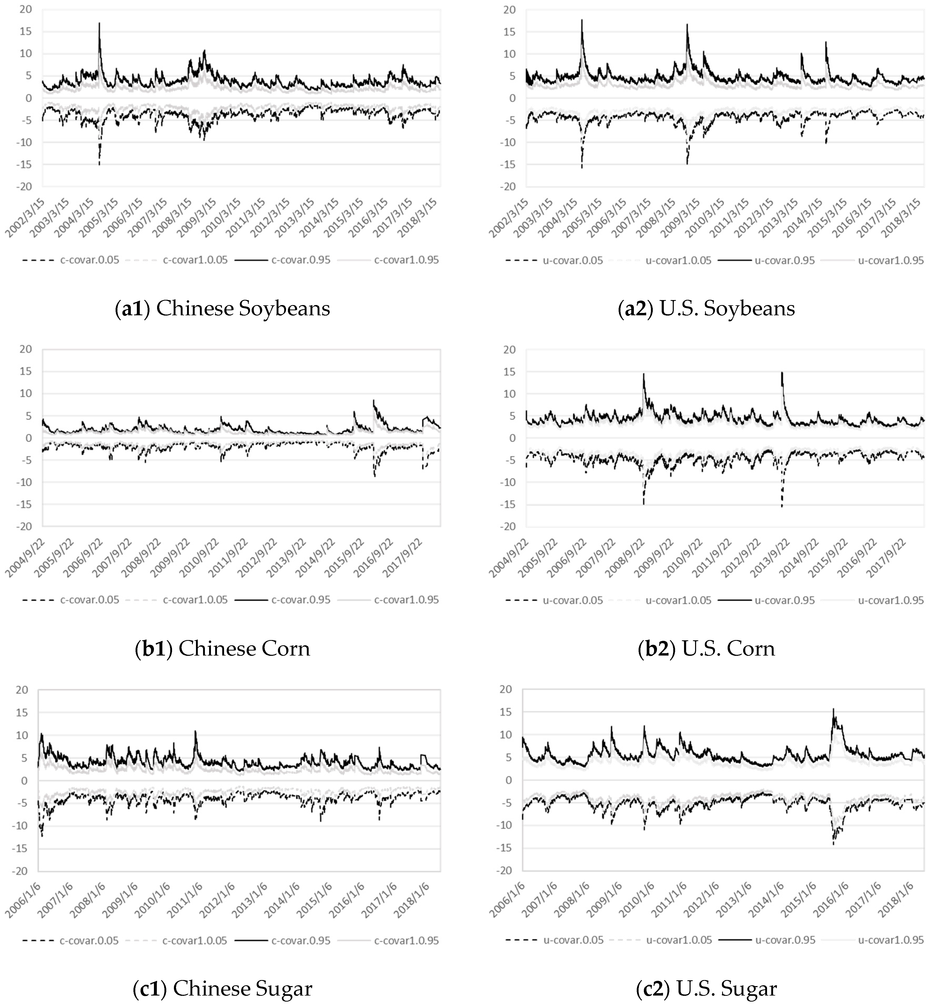
We use our BB1 copula model to calculate CoVaR and benchmark CoVaR at the 0.05 and 0.95 confidence levels to measure downside and upside risk transmission, by commodity and between exchanges, respectively. Our results are presented in Figure 4 with charts on the left-hand side depicting Chinese CoVaR levels by commodity, and the right-hand side showing U.S. CoVaR levels by commodity. We can see that CoVaR and benchmark CoVaR levels for all three commodities vary significantly over time. Notable spikes in U.S. soybeans and corn CoVaR levels, and to a lesser extent in Chinese soybean CoVaR levels, occur during the 2008–2009 commodity price boom, which was a period of extremely high price volatility. Our results highlight two interesting facts. First, we observe that the soybean CoVaR and benchmark CoVaR estimates are notably higher than the comparable estimates with respect to corn and sugar. This reflects the fact that holding soybean futures positions is associated with the greatest risk levels. Second, it is worth noting that U.S. commodity futures markets have higher CoVaR and benchmark CoVaR levels than their Chinese counterparts. This illustrates the fact that U.S. commodity futures markets are faced with a greater level of inherent risk and are subject to more extreme daily price movements.

We now turn to the question of whether risk transmission takes place between U.S. and Chinese futures markets.

Table 8. Risk transmission tests between Chinese and U.S. agricultural futures markets.

Country	Confidence Level	Soybean		Corn		Sugar
		${\mathit{T}}^{\mathit{e}\mathit{q}}$	p-Value	${\mathit{T}}^{\mathit{e}\mathit{q}}$	p-Value	${\mathit{T}}^{\mathit{e}\mathit{q}}$	p-Value
China	0.05 (downside)	26.482	0	14.434	0	21.474	0
U.S.	0.05 (downside)	25.512	0	16.910	0	15.817	0
China	0.95 (upside)	27.495	0	12.585	0	22.795	0
U.S.	0.95 (upside)	31.048	0	13.764	0	19.517	0

Note: For example, the first row presents risk transmission test results of whether there is a significant difference in downside CoVaR and benchmark CoVaR risk levels for Chinese soybean, corn, and sugar markets.

presents our risk transmission existence test results based upon the $T^{eq}$ Kolmogorov-Smirnov statistic presented in Equation (16). We find the CoVaR and benchmark CoVaR measures for the exchanges, and by each commodity, are significantly different with respect to the downside and upside risk levels. Thus, we can conclude that the downside and upside price (return) risk transmission takes place between the exchanges and with respect to all three commodities. Importantly, risk transmission is bi-directional, with price shocks emanating from both countries being transferred to each other’s markets.

3.2.2. Quantifying Risk Transmission

The risk transmission between Chinese and U.S. agricultural futures markets are next quantified using Equation (17), which calculates the percentage difference between CoVaR and benchmark CoVaR for both upside and downside, across exchanges, and by commodities. The results shown in

Table 9. Descriptive statistics of risk transmissions.

Commodity	Risk Transmissions	Downside or Upside	Average	Standard Deviation
Soybean	China to U.S.	downside	44.447	8.631
	China to U.S.	upside	61.167	5.754
	U.S. to China	downside	75.549	16.894
	U.S. to China	upside	79.668	5.450
Corn	China to U.S.	downside	34.598	2.087
	China to U.S.	upside	26.981	4.088
	U.S. to China	downside	50.876	18.194
	U.S. to China	upside	44.578	26.007
Sugar	China to U.S.	downside	29.814	2.200
	China to U.S.	upside	40.351	4.855
	U.S. to China	downside	65.834	17.163
	U.S. to China	upside	71.711	5.882

Note: Units of measurement are the percentage change in CoVaR to benchmark CoVaR in terms of daily returns.

indicate that the average risk transmission from U.S. to Chinese markets are larger than the other way around, for both upside and downside risk. In addition, it is of particular interest to note that in general, the average upside risk transmission is larger than downside risk transmission across commodities. In addition, we find that soybean risk transmissions are on average larger than sugar and corn risk transmissions for both upside and downside risk levels.

Table 10. Comparison of risk transmission for soybean, corn, and sugar markets.

Panel A Risk Transmission from U.S. to China
Risk transmission	Null hypothesis	$T^{fsd}$	p-value
Downside	corn > soybean	27.112	0
	corn > sugar	17.916	0
	sugar > soybean	23.098	0
Upside	corn > soybean	32.831	0
	corn > sugar	27.856	0
	sugar > soybean	20.489	0
Panel B risk transmission from China to U.S.
Risk transmission	Null hypothesis	$T^{fsd}$	p-value
Downside	corn > soybean	29.955	0
	corn > sugar	0.103	0.963
	sugar > soybean	38.292	0
Upside	corn > soybean	40.340	0
	corn > sugar	36.076	0
	sugar > soybean	38.007	0

presents a further comparison result of risk transmissions from the perspective of different commodities (soybean, corn, and sugar). Panel A results show that with respect to both upside and downside risk transmission from U.S. to China, soybean risk transmission is greater than corn and sugar, while sugar risk transmission is larger than corn. In panel B, results show that with respect to downside risk transmission from China to U.S., soybean risk transmission is again greater than corn and sugar, but that corn risk transmission is higher than sugar. Regarding upside risk transmission from China to U.S., soybean risk transmission is again greater than corn and sugar, while sugar risk transmission is higher than corn. Without a doubt, soybean markets experience the greatest levels of risk transmission, irrespective of where the price shock initially occurs.

Results presented in

Table 11. Comparison of upside and downside risk transmission.

Commodity	Risk Transmission	Null Hypothesis	${\mathit{T}}^{\mathit{f}\mathit{s}\mathit{d}}$	p-Value
Soybean	U.S. to China	downside > upside	17.856	0
	China to U.S.	downside > upside	33.816	0
Corn	U.S. to China	downside > upside	1.541	0.003
	China to U.S.	downside > upside	0	1
Sugar	U.S. to China	downside > upside	14.868	0
	China to U.S.	downside > upside	35.899	0

compare the relative magnitude of upside and downside risk transmission by commodity and across exchanges. First with respect to both soybeans and sugar, it is evident that upside risk transmission is greater than downside risk transmission irrespective of where the risk emanates—the U.S. or China. Turning to our corn results, we again find that upside risk transmission form U.S. to China is larger than downside risk, but that the reverse is true when analyzing risk transmissions from China to the U.S. Generally, our risk transmission results are consistent with our tail dependence results, which show that all the upper tail dependencies are larger than the lower tail dependencies.

Finally,

Table 12. Comparison of risk transmission from U.S. to China and from China to U.S.

Commodity	Risk Transmission	Null Hypothesis	${\mathit{T}}^{\mathit{f}\mathit{s}\mathit{d}}$	p-Value
Soybean	Downside	China to U.S. > U.S. to China	33.698	0
	Upside	China to U.S. > U.S. to China	39.576	0
Corn	Downside	China to U.S. > U.S. to China	31.418	0
	Upside	China to U.S. > U.S. to China	19.991	0
Sugar	Downside	China to U.S. > U.S. to China	36.091	0
	Upside	China to U.S. > U.S. to China	35.857	0

shows results with respect to which country’s exchanges transmit the larger risk levels by commodity and risk type. Importantly, irrespective of commodity and risk type—upside and downside risk—we find that U.S. exchanges transmit more risk than Chinese exchanges. This result, again highlights the fact that U.S. exchanges—in comparison to Chinese exchanges—are still playing the leading price discovery role for world agricultural commodity markets.

4. Discussion

In summary, our empirical analysis reveals three interesting findings. First, risk transmission from U.S. to China is higher than the other way around, although we find evidence that risk transmission is bi-directional with respect to all three commodities; second, upside risk transmission from U.S. to China is significantly greater than downside risk transmission from U.S. to China with respect to all three commodities; and third, soybean risk transmission is significantly larger than sugar and corn risk transmission, and sugar risk transmission is generally greater than corn risk transmission.

We argue that our empirical results can largely be explained by economic reasoning. First, with respect to our finding that risk transmission is higher from U.S. to Chinese markets we contend that this demonstrates that U.S. commodity futures markets retain their world benchmark pricing role. Underpinning this price discovery role is the relatively large U.S. share of the world physical cash market—both in terms of production and trade—in soybeans and corn, along with the fact that the U.S. (ICE) sugar futures contract was specifically designed to reflect world prices. Indeed, our results are consistent with recent research in world wheat markets, where Janzen and Adjemian [25] emphasize that price discovery is determined where informed futures trading takes place, and that this is in turn a function of futures market liquidity, and hedging effectiveness (price correlation between futures and most actively traded world cash markets). Second, with respect to our finding that upside risk transmission from U.S. to China is significantly greater than downside risk transmission from U.S. to China—across commodities—we argue that this result is consistent with Chinese government national stockpiling (NSP) agricultural policy. Third, our finding that risk transmission levels differ across commodity markets is consistent with different levels of trade and Chinese self-sufficiency in the underlying physical cash markets. China is highly dependent on U.S. soybeans and hence soybean markets exhibit the greatest levels of risk transmission. Similarly, because China relies heavily on world sugar markets, whereas it is relatively self-sufficient in corn, we observe relatively higher levels of sugar price risk transmission compared to corn price risk transmission.

5. Conclusions

In summary, over the last ten years we have witnessed unprecedented levels of growth in the Chinese agricultural commodity futures markets. This growth has stimulated researchers to investigate whether volatility spillovers still emanate primarily in U.S. futures markets or if Chinese futures markets now also play an important price discovery role in world commodity markets. We extend this body of research by examining risk transmission between the most actively traded commodity futures contracts listed on Chinese and U.S. exchanges. Using a novel Copula based CoVaR approach we uncover three interesting risk transmission results. First, we are able to confirm that U.S. commodity futures markets still play the dominant pricing role, although we also find evidence that China plays a contributing pricing role, as risk transmission is bi-directional. Second, we find that the upside risk transmission from U.S. to Chinese commodity markets is significantly greater than the downside risk transmission from U.S. to Chinese commodity markets. Third, we are able to rank the relative levels of risk transmission across our three commodities with soybeans exhibiting the greatest levels of risk transmission followed by sugar and then corn.

From a practical standpoint our results have important implications for firms engaged in world commodity trading. We show that price risk transmission occurs between U.S. and Chinese commodity markets, and as such any firms involved in the sustainable production, procurement, storage, transportation, sale, and purchase of these commodities are exposed to this risk. In particular, and given that our results show that upside price risk transmission from U.S. to Chinese commodity markets is greatest, China as a large importer of soybeans and sugar, is most exposed to this form of price risk, and should actively hedge this risk in forward and futures markets.

On a final note, we suggest potentially fruitful directions for future research. First, an important avenue to explore will be the risk management implications of our results. Specifically, to what extent could Chinese and U.S. commodity futures and options markets be used to hedge the risk transmission between commodity exchanges? Second, given the current climate of growing agricultural trade tensions between the U.S. and China, it would be informative to simulate the price risk transmission impact between U.S. and Chinese futures exchanges of potential tariffs placed on U.S. commodity exports to China.

References

- FIA. Available online: https://fimag.fia.org/ (accessed on 26 December 2018).
- Christofoletti, M.; Silva, R.; Mattos, F. The increasing participation of China in the world soybean market and its impact on price linkages in futures markets. In Proceedings of the NCCC-134 Conference on Applied Commodity Price Analysis, Forecasting, and Market Risk Management, St. Louis, MO, USA, 16–17 April 2012. [Google Scholar]
- Hernandez, M.A.; Ibarra, R.; Trupkin, D.R. How far do shocks move across borders? Examining volatility transmission in major agricultural futures markets. Eur. Rev. Agric. Econ. 2013, 41, 301–325. [Google Scholar] [CrossRef] [Green Version]
- Jiang, H.; Todorova, N.; Roca, E.; Su, J.-J. Dynamics of volatility transmission between the US and the Chinese agricultural futures markets. Appl. Econ. 2017, 49, 3435–3452. [Google Scholar] [CrossRef]
- FAO. Available online: http://www.fao.org/faostat/en/#rankings/commodities_by_country (accessed on 26 December 2018).
- BRIC. Available online: http://www.agdata.cn/ (accessed on 26 December 2018).
- Fung, H.-G.; Leung, W.K.; Xu, X.E. Information flows between the US and China commodity futures trading. Rev. Quant. Financ. Account. 2003, 21, 267–285. [Google Scholar] [CrossRef]
- Hua, R.; Chen, B. International linkages of the Chinese futures markets. Appl. Financ. Econ. 2007, 17, 1275–1287. [Google Scholar] [CrossRef]
- Du, W. International market integration under WTO: Evidence in the price behaviors of Chinese and US wheat futures. Selected Paper. In Proceedings of the American Agricultural Economics Association Annual Meeting, Denver, CO, USA, 1–4 August 2004. [Google Scholar]
- Zhang, Y.; Tong, X. Causality Diagrams for Zhengzhou Futures Sugar Prices. Math. Pract. Theor. 2012, 42, 33–40. [Google Scholar]
- Liu, C.-C. An Empirical Study on the Corn Futures Price Relevance between dec and cbot. J. Anhui Agric. Sci. 2009, 37, 899–903. [Google Scholar]
- Jiang, H.; Su, J.J.; Todorova, N.; Roca, E. Spillovers and Directional Predictability with a Cross-Quantilogram Analysis: The Case of US and Chinese Agricultural Futures. J. Futures Mark. 2016, 36, 1231–1255. [Google Scholar] [CrossRef]
- Liu, Q.; An, Y. Information transmission in informationally linked markets: Evidence from US and Chinese commodity futures markets. J. Int. Money Financ. 2011, 30, 778–795. [Google Scholar] [CrossRef]
- Adrian, T.; Brunnermeier, M. CoVar; Federal Reserve Bank of New York Staff Report, no. 348; Federal Reserve Bank of New York: New York, NY, USA, 2011. [Google Scholar]
- Girardi, G.; Ergün, A.T. Systemic risk measurement: Multivariate GARCH estimation of CoVaR. J. Bank Financ. 2013, 37, 3169–3180. [Google Scholar] [CrossRef]
- Bernal, O.; Gnabo, J.-Y.; Guilmin, G. Assessing the contribution of banks, insurance and other financial services to systemic risk. J. Bank Financ. 2014, 47, 270–287. [Google Scholar] [CrossRef]
- Abadie, A. Bootstrap tests for distributional treatment effects in instrumental variable models. J. Am. Stat. Assoc. 2002, 97, 284–292. [Google Scholar] [CrossRef]
- Karimalis, E.N.; Nomikos, N.K. Measuring systemic risk in the European banking sector: A Copula CoVaR approach. Eur. J. Financ. 2018, 24, 944–975. [Google Scholar] [CrossRef]
- Sklar, M. Fonctions de repartition an dimensions et leurs marges. Publ. Inst. Statist. Univ. Paris 1959, 8, 229–231. [Google Scholar]
- Patton, A.J. Modelling asymmetric exchange rate dependence. Int. Econ. Rev. 2006, 47, 527–556. [Google Scholar] [CrossRef]
- Reboredo, J.C.; Ugolini, A. Systemic risk in European sovereign debt markets: A CoVaR-copula approach. J. Int. Money Financ. 2015, 51, 214–244. [Google Scholar] [CrossRef]
- Reboredo, J.C.; Rivera-Castro, M.A.; Ugolini, A. Downside and upside risk spillovers between exchange rates and stock prices. J. Bank Financ. 2016, 62, 76–96. [Google Scholar] [CrossRef]
- Brorsen, B.W.; Ji, D. A relaxed lattice option pricing model: implied skewness and kurtosis. Agric. Financ. Rev. 2009, 69, 268–283. [Google Scholar]
- Mondovisione. Available online: http://www.mondovisione.com/media-and-resources/news/fia-releases-summary-statistics-for-2017-futures-and-options-volume-and-open-int/ (accessed on 26 December 2018).
- Janzen, J.P.; Adjemian, M.K. Estimating the location of world wheat price discovery. Am. J. Agric. Econ. 2017, 99, 1188–1207. [Google Scholar] [CrossRef]
Figure 1.
Annual volume of futures contracts traded in Chinese and U.S. futures exchanges (2013–2016), ICE here refers to ICE Futures U.S., which is a member of the Intercontinental Exchange. Source: FIA [1].
Figure 2.
Daily closing prices of soybean, corn, and sugar futures contracts in China and U.S., the unit is yuan/ton. Source: Bric [6].
Figure 3.
Time-varying upper and lower tail dependence coefficients between Chinese and U.S. agricultural futures markets implied by BB1 copulas.
Figure 4.
Dynamic conditional value at risk (CoVaR) and benchmark CoVaR of soybean, corn, and sugar returns. Note: c-covar and c-covar1 refer to Chinese market CoVaR and benchmark CoVaR measures calculated using and . On the other side, u-covar and u-covar1 are the CoVaR and benchmark CoVaR of U.S. market calculated with and .