“BalSim”: A Carbon, Nitrogen and Greenhouse Gas Mass Balance Model for Pastures


1
MARETEC – Marine, Environment and Technology Centre, LARSyS, Instituto Superior Técnico, Universidade de Lisboa, 1049-001 Lisboa, Portugal
2
Centre for Ecology, Evolution and Environmental Changes (cE3c), Faculdade de Ciências da Universidade de Lisboa, Campo Grande, 1749-016 Lisboa, Portugal
3
ICAAM, University of Évora, Núcleo da Mitra apartado 94, 7006-554 Évora, Portugal
*
Author to whom correspondence should be addressed.
Sustainability 2019, 11(1), 53; https://doi.org/10.3390/su11010053
Submission received: 1 October 2018
/
Revised: 14 December 2018
/
Accepted: 18 December 2018
/
Published: 21 December 2018
(This article belongs to the Special Issue Livestock Production and Industrial Ecology)
Abstract
:Animal production systems are increasingly required to co-produce meat products and other ecosystem services. Sown biodiverse pastures (SBP) were developed in Portugal as an improvement over semi-natural pastures (SNP). SBP increase yields and animal intake during grazing, are substantial carbon sinks, and the abundance of legumes in the mixtures provides plants with a biological source of nitrogen. However, the data available and the data demands of most models make integrated modelling of these effects difficult. Here, we developed “BalSim”, a mass balance approach for the estimation of carbon and nitrogen flows and the direct greenhouse gas (GHG) balance of the two production systems. Results show that, on average, the on-farm GHG balance is −2.6 and 0.8 t CO2e/ha.yr for SBP and SNP, respectively. Ignoring the effects of carbon sequestration, and taking into account only non-CO2 emissions, the systems are responsible for 17.0 and 16.3 kg CO2e/kg live weight.yr. The annual analysis showed that non-CO2 emissions were highest in a drought year due to decreased yield and stocking rate. We also showed through scenario analysis that matching the grazing level to the yield is crucial to minimize emissions and ensure reduced feed supplementation while maintaining high soil carbon stocks.
1. Introduction
The idea that current global production patterns of animal products, meat, in particular, are unsustainable gained popular support and media attention following the 2008 “Livestock’s Long Shadow” report [1]. The report pinpointed livestock production as one of the main sources of greenhouse gases (GHG), responsible for 8–18% of global emissions [2], mostly due to emissions from animals and manure, and the production of concentrate feed [3]. The global per capita consumption of meat grew from 38.9 kg to 42.2 kg between 2005 and 2011 and is expected to grow 1.3% per year until 2050 [4], in spite of dietary changes in developed countries. Therefore, supply-side environmental optimization will be crucial in the near future. Dominant global animal production systems must change to cope with future demand sustainably, and there is room for improvement. Among other requirements, improvement should leverage the potential of animal systems to supply ecosystem services. Extensive grass or grass/legume-based systems use marginal land for grazing [5], accelerate nutrient recycling [6], and can sequester carbon (C) in soils [7]. For example, sown biodiverse permanent pastures rich in legumes (SBP) in Portugal are a win-win meat production system for the economy and the environment [8,9]. SBP are self-reseeding grass-legume pastures with up to 20 native and high-yielding species/cultivars with an annual life cycle. They increase grassland productivity and sustainable stocking rates [7]. The abundance of legumes ensures a natural source of nitrogen (N) for pasture growth. The high yields and the annual cycle of the plants ensures a high input of C into the soil, and consequent C sequestration. A scheme for payments for C sequestration services in SBP was set up by Terraprima with the support of the Portuguese Carbon Fund (PCF) in 2009–2014. More than 1000 farmers were paid by for the C they sequestered. SBP now occupy more than 4% of the country’s agricultural land [8,10]. They can therefore be a prime example of how to improve the sustainability of meat production systems.
Accurate knowledge of how C and nitrogen (N) flow through these pasture ecosystems is essential to understand both the sources of GHG emissions (which influence emissions of the main GHGs—CO2, CH4 and N2O) and minimize them, and to study how grazing can influence nutrient cycling in ecosystems [11,12]. SBP have been the subject of experimental research mostly on their capacity to sequester C in soils [12,13]. A full assessment of how C and N flows in and out of SBP parcels and of semi-natural pastures (SNP), the alternative systems that SBP commonly replace, has never been carried out. The entire GHG budget of these systems, apart from simple applications [12,14], remains unknown. This is critical because even if installing SBP in formerly less productive SNP sequesters C in soils, there could potentially be increased emissions that counteract that effect. Additionally, from the farmer’s standpoint, the main variables of interest in the pasture production system, because they represent performance, are the stocking rate which can be sustained by the pasture at its current yield (potential number of animals that can sustainably be fed in a certain area) and now also C sequestration. Besides the agronomic benefits of C sequestration on fertility and water management, C became an additional potential service provided by farmers during the PCF project. Those farmers need tools to assess the interplay between agronomic and environmental performance.
The most promising ways to overcome these gaps in knowledge are to either measure all these flows or use models. Measuring is expensive and time-consuming, as it requires determining individual flows from all components of the pasture system, including animals. It may also be redundant, as there is plenty of published experimental research for related systems. Modelling is thus an option, but then the question becomes the desired level of detail. Process-based models would be very accurate but require even more site-specific data to estimate these flows [15]. Simple mass balance models such as the OECD soil surface nitrogen balance [16] would be more manageable but also too simple to provide actionable insights about pasture management and how it can influence emissions. The optimum procedure should not only be descriptive but also prescriptive—it should inform researchers and farmers about what to do to maximize production and environmental performance. It should also be specific for the system, but not so complex that it requires data even more difficult to obtain than measuring GHG and nutrient flows directly. To our knowledge, despite the high number of tools available to perform similar calculations, no available tool meets exactly those conditions.
In this paper we propose a mass balance approach based on the OECD model, but tailor-made for this application at the level of detail that fits the limited available data on SBP. The integrated model, “BalSim - Carbon and Nitrogen Mass Balance Simulator”, includes two interconnected mass balance models, for C and N, applied for each balanced sub-system within the pasture system, which also enable the determination of the GHG balances. Our goals for this paper were to (a) develop BalSim as a working model of C and N flows in SBP and SNP ecosystems, (b) demonstrate the applicability of the model to calculate the GHG balance of each system, and (c) test the capacity of the model to provide meaningful insights for pasture management. The goal of BalSim is to rely on limited farm data so that, in the future, it can be used for research and by farmers to test the effects of management on the agronomic and environmental performance of these pasture systems. In the sections that follow, after establishing the models, we apply them for animal production in average SBP and SNP. Based on this analysis, we calculate the GHG balance of the two pasture systems. We also perform a dynamic analysis for four years of measured yield, stocking rate and soil C data. We test three scenarios that farmers may face when managing these pastures, to understand whether BalSim is capable of providing useful answers. Finally, we provide several suggestions for how the model can be improved in the future.
2. Materials and Methods
2.1. Study Sites
In this work we used data from the AGRO 87 project [17] to characterize the two systems under analysis: SBP and SNP. This project ran between 2001 and 2005 in six farms in Southern Portugal (Alentejo) where both pasture systems used in this work co-exist. The study farms had grazing suckle cows for meat production. Varying amounts of supplemental feed were provided to the animals, but the type (concentrate, roughage) and amount were not measured. The project used SNP parcels and divided them into two, where the SBP were installed in one half. Each system occupied a contiguous 14 ha plot. There were no significant differences between plots in terms of topography, soil characteristics or prior history of the parcels. In both systems, there was no nitrogen fertilization. A full biophysical and technical characterization of the two systems studied, SBP and SNP, was produced by Teixeira et al. [8]. The farms were: farm 1 (H. Cabeça Gorda—near Vaiamonte); farm 2 (H. Monte do Mestre—near Elvas), farm 3 (H. Claros Montes—near Pavia); farm 4 (H. Refróias—near Santiago do Cacém), farm 5 (H. Cinzeiro e Torre—near Coruche) and farm 6 (Quinta da França—near Covilhã). The location of these farms can be seen in Teixeira et al. [7]. These regions are classified as hot-summer Mediterranean climate region, according to the Köppen climate classification [18,19]. The main climatic characteristics of farms were similar between 1981 and 2010, with monthly average temperature of 11–17 °C and yearly precipitation of 585–945 mm [19]. Despite the number of years past since the project ended, it remains the most comprehensive experimental assessment made of SBP and their comparison with SNP. The project measured (a) the yield, (b) actual stocking rates, (c) soil organic matter (SOM) and other soil parameters, and (d) the floristic composition of the pastures, namely the percentage of coverage with grasses and legumes. Unfortunately, these parameters were not consecutively measured for all years in all farms.
2.2. Available Data on the Two Pasture Systems
Table 1 shows the averages for all years of the project for SNP and SBP of aboveground grass productivity, stocking rate, grazing time, SOM concentration and air temperature [8]. These were the only measured variables used in the present paper. Data per farm and year are presented in online Supporting Supplementary Materials file S1. The methods used for data collection are presented in the project report [17] and summarized in the previous literature that used data from the same project [7,8,14,20,21]. For stocking rate, we considered that each livestock unit (LU) can be partitioned between one adult cow (1 LU/head) and a corresponding less than one-year old weaner calf (0.4 LU/head). The calf can be either female or male. Young heifer calves are used as replacement cows, while steer calves are used for meat. The adult animal should be included as it was required to give birth and partially feed the calf until weaning and was also present on the same plots grazed by the calf after weaning.
2.3. C and N Mass-Balance Model Development
The model BalSim comprises three sub-systems: plant, livestock and soil. Each sub-system includes several pools, which are defined as elements where the C and N balance of inflows, outflows and accumulation must be equal to zero. Mass transfers between pools are translated by flows, which are then described in terms of their C and N contents. Each flow and variation of stock (for accumulations) is presented in Table 2. Flows and stock variations are designated in this paper as variables. The model explicitly includes all GHG emissions as outflows. The balance equations for each pool are described in Table 3.
We applied the BalSim to the pastures sites and systems described in Section 2.1 by using the measured data in Table 1 in combination with additional parameters collected from the literature. Figure 1 visually depicts the flows and pools included for this system. The systems under analysis in this work do not consider mass flows for manure (i.e., organic C and N exported from the field due to time spent by the animals in household or yards. Consequently, we did not consider manure storage either because animals graze 100% of the time. The physical boundaries of the analysis were therefore set at the pasture plot, where the animals graze. Also, no C or N enters the system through fertilization because these pastures do not require organic fertilizers or inorganic N fertilizers. The temporal boundary selected was one year.
To quantify each variable of the model, we used a combination of the measured data and additional parameters, which were collected as much as possible from the specialized literature on SBP or similar systems. A description of the quantification procedure for each variable in each sub-system is provided in the next section. First, the model was applied using the average of all years and farms in Table 1 (as described in Section 2.3.1, Section 2.3.2 and Section 2.3.3, with additional analyses described in Section 2.4, Section 2.5 and Section 2.6), and then annually (described in Section 2.7). Table 4 presents the parameters that were collected from the literature and are involved in the calculation of all flows, in combination with the four measured parameters indicated in Table 1.
2.3.1. The Plant Sub-system
Pasture plants take up C via photosynthesis ( from Table 2) and N through nutrient uptake from the roots (). The accumulation of both elements in the above and belowground of the plant was considered null, because of the annual cycles of the plants in these pastures (particularly SBP). During each year, aboveground plants are either eaten by livestock () or become litter (where in this paper “litter” is a simple designation for plant materials unused for animal feed, e.g., due to leaf senescence). The part that becomes litter can enter the soil (), together with roots (), or be lost due to emissions (). In situ dry matter (aboveground) productivity () was the only measured input data available that is usable in this sub-system (Table 1). Note that, in our application, the variable is the net uptake of C from photosynthesis by the plant, i.e., it considers the reemission of C due to plant respiration. We did not consider any accumulation of plant biomass between two years. SBP plants have a truly annual cycle, as they germinate in the autumn and die out through the summer, self-reseeding from the seed bank established during spring. Furthermore, it is good management to ensure that during the summer the pasture is fully grazed to allow for spontaneous germination of the sown species, particularly legumes, during autumn. Farmers received technical advice and were likely to have followed this practice. For SNP we had no data to estimate inter-annual accumulation of plant biomass, and assumed it as a simplification to be zero.
We started by converting (indicated in Table 1) into aboveground C and N using the C and N content of grasses and legumes. The unit contents used were 0.45 kg C/g DM and 0.02 kg N/kg DM, respectively, for SBP, and 0.35 kg C/g DM and 0.01 kg N/kg DM for SNP, and calculated as follows. The C content for SBP used was the average for grass and legume species (assuming 50%/50% DM production of grasses/legumes), which typically ranges between 0.35 and 0.50 kg C/g DM [22]. The N content for SBP was obtained as the average content of grasses and legumes [32] (which is 0.00868 and 0.0283 kg N/kg DM, respectively). The N content of SNP, where legumes are almost non-existent, was an approximation of the N content of grasses, while the C content was the minimum C content in grasses. Implicitly, these numbers assume that the aboveground plant C:N ratio is approximately 24 for SBP plants and 40 for SNP plants.
The average fraction of the yield that becomes litter () in SBP for the stocking rates used (Table 1) was 0.39. This number was estimated during the calibration of the Rothamstead Carbon model (RothC) [33] for the same farms and years used in this paper (Table 1) [21]. For SNP there was no data available, so we assumed as a simplification that the fraction of litter was equal to for SBP multiplied by the ratio of yields between the two pasture systems, i.e., approximately 0.62. We assumed equal chemical composition of plants (aboveground) and the litter. Therefore, C and N contents for litter were obtained by multiplying the amount of litter and the C and N contents mentioned above. The fraction of the yield that is not litter is the fraction eaten by the animals, which can be calculated using
The accumulation of the litter pool is also considered null, since it is assumed that after one year all litter has been incorporated into the soil matrix (fraction represented by and ) or converted into atmospheric emissions. Some C and N are lost through atmospheric emission of CO2 and N2O, which occur due to the organic decomposition and nitrification processes on litter material. N2O emissions from litter () were calculated using an emission factor of 0.0049 kg N-N2O/kg N litter [23] that takes into account the N content of the litter fraction as
We assumed that the decomposition of litter only produces N emissions as N2O (in accordance with EMEP/EEA [23]). CO2 emissions from litter (), due to the absence of a source for their determination, were calculated as a stoichiometric balance starting from N2O emissions assuming that the C:N ratio of the litter does not change after N2O emissions (i.e., multiplying by ).
Then, we converted into belowground production using literature values for rroot:shoot and C and N contents of roots. The was obtained from the same source as [21]. C and N contents of roots were, respectively for SBP and SNP, 0.45 and 0.35 kg C/g DM, and 0.03 and 0.01 kg N/kg DM [32]. In SBP, the C and N contents were calculated as an average of likely root C and N contents for grasses and legumes (0.37–0.52 kg C/g DM; 0.01–0.05 kg N/kg DM) [34]. For SNP, the contents were estimated by assuming that they should be equal to the content for SBP multiplied by the ratio between below and aboveground contents in SBP. Implicitly, we thus assumed that the C:N of roots is 15 and 25 in SBP and SNP respectively.
2.3.2. The Livestock Sub-system
The livestock sub-system involves two balances – the balance to the animal, and the balance to the excreta (dung and urine). The total number of animals in the pasture varies according to the stocking rate of each farm, which was measured and is indicated in Table 1 (). The inputs of the animal balance are the intake from the pasture () and from the supplemental feed (). In SNP, the animals require feed due to the limited grass yield. In SBP, animals require supplemental feed during particular months of the year when pasture yield is limited by temperature (e.g., winter) or water availability (e.g., during the summer). Feed supplementation in SBP is also necessary due to the fact that grazing should be maximized before Fall to decrease ecological competition against the more interesting sown species (particularly legumes), avoiding the establishment of less nutritive or even woody plants and making way for the seeds of the originally sown plants to germinate. There is accumulation of C and N in the tissue of the body of the animals (), who excrete C and N (). The animals also breath out CO2 () and emit CH4 from enteric fermentation ().
Regarding the inputs, was obtained from Equation (1). The amount of N in the feed () was calculated using the animal N balance. After determining this parameter, we converted it into using a C:N ratio of the feed of 19.53 [22], and assumed the same type of feed was provided to animals in both systems, according to
The carbon and nitrogen accumulation in the animal body was calculated through estimates of animal growth (289.9 kg live weight/LU calf.yr [24]) and the C and N contents of live tissues (0.487 kg C/kg live weight and 0.114 kg N/kg live weight [25]). We assumed the same type of animal and growth in both pasture systems. It was also necessary to take into account the water content in the bodies, estimated as 65% [35], and the difference between adult cows and calves because only calves accumulate body weight, as adult cows are already at maturity. This is expressed as
where the stocking rate for calves () in LU took into account the contribution of cows (βcow =1) and calves (βcalf = 0.4) [17] for the total stocking rate in each pasture system (5), meaning
The output concerning the amount of N excreted by the animal () has been established in literature and was therefore used in this study. Total excretion of N is a weighted average of excretion factors (105 and 44 kg N/ha.yr for cows and calves, respectively [23]) for and the stocking rate of adult cows (), which means that
Carbon excretion () was then obtained assuming a C:N ratio of the excreta (dung + urine) of 19.1 [26].
In the livestock sub-balance, the atmospheric emissions are significantly different because the cows release some C in the form of CO2 and CH4 from respiration and enteric fermentation respectively, while in the N balance there are no atmospheric emissions released by the animal.
CH4 emissions from enteric fermentation are calculated using emission factors for cows and calves while the CO2 resulting from animal respiration remains as the only unknown of the C balance for animals, as expressed by
The emission factors for CH4 used were 81.3 kg CH4/head.yr (the average of the interval 75.9–86.7 kg CH4/head.yr) for cows, and twice of 19.6 kg CH4/head.yr (the average of 18.3–20.9 kg CH4/head.yr) for calves [27] because the original emission factors consider that calves only spend 6 months in the pasture—in our case, they spend double that time.
For excreta a simple balance can be established. Out of the amount excreted by animals (), a fraction ends up on the field (), and the rest is emitted to the atmosphere – in the case of C, in the form of CO2 () and CH4 (); for N, in the form of N2O () and NH3 (). We assumed no accumulation of the dung and urine excreted in the field, since everything that is not emitted enters the soil pool.
The amounts of C and N excreted are a result of the animal sub-balance. The emissions of N2O were calculated using the emission factor 0.02 kg N-N2O/kg N during grazing [27]. The emissions for NH3 from dung and urine are calculated using emission factors for cows and calves (0.1 and 0.06 kg N-NH3/kg N dung, respectively [23]). The only unknown in the N balance for dung is therefore nitrogen flow of urine and dung going through decomposition in the soil, and entering both the organic and inorganic N soil pools, calculated as
In the carbon cycle, CH4 emissions from dung and urine were calculated using an emission factor of 13 kg CH4/LU.yr [28], duly converted into emissions per hectare using the stocking rate. In the case of C, we assumed that all material excreted by the animal is organic. Finally, CO2 emissions are calculated using the mass balance equations, since it remains as the only unknown, as
2.3.3. The Soil Sub-system
There are three pools and respective balance equations in the soil – the C organic pool, and the N organic and inorganic pool. We excluded a C inorganic pool due to its limited interaction with the organic pool that generates the most important GHG flows.
Regarding the C and N organic balances, their inputs come from the plant sub-system, namely root () and litter () decomposition, and from the animal balance, namely the input from dung and urine ( and ). There is accumulation of C and N as soil organic carbon (SOC) and nitrogen within soil organic matter (SOM). The accumulation of organic C was calculated using the measured SOM concentrations (Table 1) and the soil bulk density (1.34 g/cm3 [29]), considering the first 10cm of soil (), and that 58% of SOM is SOC, or
The conversion of the accumulation of C into accumulation of N was estimated using 19.695 for SBP and 31.955 for SNP as the C:N of soils. The selection of the C:N of soils was made through calibration in order to obtain the correct partition between organic and inorganic N from the balance. The only unknown in the soil organic N pool is , which was calculated as
The total was already pre-determined from the animal balance. Therefore, the parameter is simply the difference between the last two. However, there is a restriction on this parameter, because approximately 60% of N excreted to soils is mainly urine and should be inorganic [23]. The only parameter that can be adapted in the organic N soil balance is accumulation through the C:N ratio, and as such this parameter was adjusted until the proportion between inorganic and organic N from excreta was equal to 0.6/0.4.
The two main outputs for the organic pool are erosion () and mineralization (). The amount of C and N lost by erosion was calculated using estimates of soil loss per hectare (estimated as 1.03 t soil/ha in the region of the farms [30]) and respective amounts of C and N in soils. Mineralization of SOM leads to CO2 emissions that were calculated using the carbon mass balance equation
Mineralization of SOM also produces NH4+ that enters the soil inorganic N pool. This was calculated using the amount of C lost during bacterial decomposition and the C:N of soils, thus implying an assumption that there is no change in the chemical composition of SOC throughout the year.
For the soil inorganic N pool the inputs are N inbound from the organic pool due to mineralization (), manure decomposition () and also N from atmospheric deposition () and N captured in root nodules by rhizobia following seed inoculation and/or free-living N fixing microorganisms (). Atmospheric deposition was quantified using a factor of 1.06 kg N/ha [14]. N fixation was estimated using the amount of N fixed of 0.026 kg N fixed/kg DM [27]. This should provide a fixation of approximately 180 kg N/ha [17].
The outputs of the inorganic N pool are the amounts of N taken up by plants determined in the plant balance (), and also atmospheric emissions of N2O from soils () and due to the biological fixation of N (). The emission of N2O resulting from nitrification processes occurring in the soil is calculated using the air temperature (Tair), which is available for the farms (Table 1) and empirical parameters adapted to grassland land use types [36] according to
where is a factor dependent on land use cover, which in this case is 0.9 ngN/m2.s [36]. If legumes are also present, as is the case of SBP, we used also the N2O emission factor 0.0125 kg N-N2O/kg N fixed [31].
The remaining unknown is residual inorganic N that could be (a) inorganic N accumulating in soil, or (b) inorganic N loss through leaching (to groundwater or deeper soil depths). To avoid overcomplicating the model, we designated this residual inorganic N of the balance equation as , and calculate it as the unknown using
2.4. Verification of Average Results
As the variables indicated here were not measured for these systems, farms and years, we were unable to validate results using plot-level data. Therefore, we performed indirect verification using three main parameters: (a) the amount of feed supplementation provided by the model; (b) the closure (i.e., net loss/gain) of the organic C soil model, and (c) the closure of the inorganic N model.
Regarding the level of feed supplementation estimated by the model, it should correspond to approximately 0.5–1.5% of the live weight of the animals per day in SNP [14,37]. These percentages correspond to 381–1142 kg feed DM/ha, considering the stocking rate of SNP.
The organic C soil balance is closed by calculation of . An independent estimation of this parameter states that it should be approximately 13% of the average SOM, duly converted to C [21].
For the inorganic N soil balance, it would be expected that the residue term was zero. There is some evidence of limited to no loss of NH4 in SBP [38]. There may be, however, a small accumulation of NO3 of up to 30 kg N/ha [38]. SNP plant growth is limited by N availability, and consequently little to no loss or accumulation of inorganic N is expected.
2.5. Greenhouse Gases Balance Calculation
The GHG balance (t CO2e/ha.yr) was calculated for the average of all years and farms in Table 1 by all the inbound and outbound flows of C and N gases linked to greenhouse effects, considering the entire plant + animal + soil sub-systems. The inflow of CO2 occurs through photosynthesis and the outflows include CO2 emission from litter and mineralization together with animal respiration. The outflow of CH4 gas includes animal enteric fermentation and emissions from dung and urine excreted by animals in the field. Finally, N2O gas outflow from the system includes emissions from litter, dung and urine decomposition, and soil emission through nitrification processes and also includes the biological fixation of N, in SBP. The balance is, therefore, calculated as:
where the C and N fluxes were converted into emissions using the respective molecular/atomic weights and converted into CO2e using the IPCC global warming potentials (GWP) including climate feedbacks [39] ( = 1, = 34, = 298).
Equation (16) was simplified by including only non-CO2 GHGs as
This assessment excludes the contribution of CO2 emitted that had been previously captured by the plants during photosynthesis (17). It also assesses emissions without the offset from C sequestration in SBP, which is known to be large [7] and can therefore dominate the calculation in Equation (16). The emissions calculated in Equation (17) were then converted from kg CO2e/ha into kg CO2e/kg of live weight of the animal, using the weight of the calf at the end of the year of analysis. In this analysis we assumed that the calf was a steer.
2.6. Scenarios
BalSim should be useful for farmers to test the results of management on the agronomic and environmental performance of the pasture systems. To test the capacity of the model to address real agronomic questions in relation to their outcomes, three scenarios were tested using the model developed here. Each scenario corresponded to a question, namely:
S1—In a good year, where yield doubles and farmers also double the stocking rate, if there is no extra feed supplementation, what would be the increase in SOM?
In this scenario we doubled the average productivity and stocking rate (from Table 1) while the other parameters remained constant except for the average SOM concentration. We assumed that, for soils to sustain such high yields, they would have to be extremely productive and rich in SOM, and as such used the highest observed SOM concentrations over all of the years in which it was measured in SBP and SNP of 5.6% and 4.7%, respectively [17]. We then changed the annual SOM increment until the soil organic C model was balanced.
S2—If we aim to double the annual SOM increase, what is the necessary yield and stocking rate?
In this scenario we doubled SOM increases (from Table 1) while the other parameters remained constant. We then changed yield and stocking rate until the model was balanced.
S3—In a poor agronomic year where yield is only half, if farmers want to maintain SOM increases and maintain their average feed supplementation, what is the maximum sustainable stocking rate?
This scenario assumed that the average yield (from Table 1) was halved while the other parameters are the same, including the SOM increase and feed supplementation. The stocking rate was then adjusted until the model was balanced.
2.7. Annual Application of the Model
The model and all calculations, including the GHG balance, were also performed on an annual basis using data for 2001–2005 for SBP (using annual data in online supporting materials file S1). The annual analysis did not include SNP due to lack of annual data for most farms. For this application, we used the annual yield, stocking rate, SOM and SOM increase of SBP, plus the average annual air temperature, for each year.
For each year, all parameters in Table 4 were kept constant except three: (a) the , (b) the rroot:shoot, and (c) the C:N of the soil (in order to maintain the relationship between organic and inorganic input to soil from dung and urine). We adjusted these three parameters until the soil organic C balance was equal to the expected [21] (explained in Section 2.4) and recorded the final values. The annual GHG balance was also calculated.
3. Results and Discussion
3.1. Average SNP and SBP Systems
Results in this section were obtained using the averages for all farms and years presented in Table 1.
3.1.1. Evaluation of the Parameters Used
The C content in the aboveground biomass usually ranges between 0.30 and 0.50, and the N content in the aboveground biomass between 0.02 and 0.15, according to pasture chemical analysis [22] depending on the type and species in the pasture. The parameters we chose are within this range. Regarding the parameter , literature values for pastures can range between 0.5 and 9. For grasslands in the region of Alentejo, which are classified according to the Moderate Resolution Imaging Spectroradiometer (MODIS) [40] as “temperate arid shrubland”, the is 1.063 [28,41]. We used 0.98, which besides being consistent with this estimate was obtained from an optimization process using the same input data used in this paper. Finally, is highly dependent on the feed ingredients and whether the supplemental feed is concentrate or roughage. The most common value is about 20, but for the most common concentrate ingredients the C:N ranges between 15 and 30 (e.g., 15 for olive husk and 29 for maize grain). According to Matschullat et al. [42], the in agricultural and grazing areas in the Alentejo region is higher than 18. All parameters used in this paper are within these ranges.
3.1.2. Carbon and Nitrogen Flows
Figure 2 shows that the amount of C and N from the pasture biomass ingested by the animals was, for C, more than triple in SBP compared to SNP (1680 and 456 kgC/ha.yr) and, for N, more than 6 times higher in SBP (69 and 11 kg N/ha.yr). The combined flows of the plant and litter pools were also higher in SBP when compared to SNP. Root decomposition is the main outflow from the plant sub-system–2669 (SBP) and 2543 kgC/ha.yr (SNP) and 180 (SBP) and 51 (SNP) kg N/ha.yr respectively. Litter decomposition was particularly high for SNP in C with a contribution of 829 kgC/ha.yr, while nitrogen was less than half of what was decomposed in the SBP. N2O (in kg N/ha.yr) emissions represented around 0.2% of the respective N inflow for the plant balance in both pasture systems, thus playing a small part in the mass balance calculation.
Inputs into the animal pool include not only the pasture ingested during grazing, but also the supplemental feed intake, which is higher in the SNP than in the SBP, both in carbon (302 and 471 kg C/ha.yr) and nitrogen (15 and 24 kg N/ha.yr), despite the fact that stocking rates are much lower in SNP. The biggest contributor in terms of mass outflow is the animal excretion through urine and dung, which represents 70–78% of the intake in carbon in SBP and SNP and 96% of the intake in nitrogen. CO2 emissions through respiration are 18% and 27% of the intake in SBP and SNP, while enteric fermentation contributes 2% (in C) in both pasture systems. The accumulation in the animal body was 13 and 6 kg C/ha and 3 and 1 kg N/ha in SBP and SNP respectively.
Emissions of CO2 resulting from the dung and urine excreted represented 11% and 5% of the excreted material in the field in SNP and SBP respectively, and CH4 was 1% for both pasture systems. N2O emissions were also higher in SBP (11%) compared to SNP (6%). However, the main flow was urine and dung that enters the soil organic and inorganic pool, both in C and N.
The soil organic C pool accumulated a total of 2,339 and 777 kg C/ha in SBP and SNP respectively. The main inflow in both systems was C from root decomposition (52% and 46% of the total inflow in SBP and SNP). The same occurred in the organic N pool, with an accumulation of 115 and 24 kg N/ha in SBP and SNP respectively and the root decomposition contribution as high as 71% and 60% in the same systems. The main outflows were the mineralization of SOM in both pasture systems for C (originating CO2 emissions, 2774 and 1910 kg C/ha.yr) and N, and NH4+ that is ready for plant uptake or nitrification (137 and 60 kg N/ha.yr).
In the inorganic N pool there is a major difference between the two systems. SBP gain from a high contribution from legume fixation (159 kg N/ha.yr) and 341 kg N/ha.yr from SOM mineralization, besides the inorganic part of dung and urine that enters the soil. SNP systems only have 80 kg N/ha.yr at their disposal. The outflows of this pool are again for both systems totally dominated by the plant uptake, since N2O emissions from the soil and the legume plants, if existing, represent only 1–2 kg kg N/ha.yr.
It is also visible in Figure 2 that the largest C and N flows are related with the plant (C input from photosynthesis, N intake from soil, root decomposition into the soil, etc.) or with the soil organic sub-system (accumulation and mineralization). Measured field data was used to estimate all these flows. Flows that were estimated from secondary sources without influence from the data in Table 1 are relatively small in terms of C and N – although they can be relevant for the results of the GHG balance explained next.
3.1.3. Greenhouse Gases Balance
The results for the GHG balance in Figure 3, show that while the SNP system is a net emitter, with 792 kg CO2e/ha, the SBP system captured 2644 kg CO2e/ha. The major contributions for the emissions in both systems are soil mineralization (59% and 69% of the total emissions respectively) and both animal respiration and enteric fermentation representing up to 7–12% in SBP and 9% in SNP. The rest of the emissions individually account for less than 7% of total emissions.
The different result achieved in the two systems is a direct consequence of more than the double SOC accumulation in SBP (8578 kg CO2e/ha.yr) compared to SNP (2850 kg CO2e/ha.yr), while SOM mineralization emissions from SBP represented only 1.5 times the emissions of SNP.
Considering only non-CO2 emissions, we obtained results shown in Table 3. The most relevant flow is CH4 emissions from enteric fermentation in Table 5, which alone accounts for 43% of all emissions in SBP and 45% in SNP. Emissions per hectare are higher in SBP due to the fact that the stocking rate is more than double than in SNP. However, emissions per LU and live weight of the animal are almost equal (e.g., 17.0 vs. 16.3 kg CO2e/kg LW).
3.2. Verification of Average Results
The amount of N ingested by the animals according to the N balance is equal for both systems at 0.249 kg N intake/LU.day. This was due to the fact that we assumed that the animals grew by the same amount in both systems. N is connected with important diet parameters such as protein, and as such it should be the same for all systems. Regarding consumption from feed alone, results of the application of the balance revealed that the difference in the feed required in both systems, when converted to DM, is approximately 1962 kg DM/LU.yr. When applied to the SR for SNP, this would result in an extra feed consumption of 769 kg DM/yr, which is equivalent to a 1% supplemental feed intake per day, and therefore within the plausible range for these pastures.
Regarding the closure of the organic C soil balance, if the 13% mineralization rate had been used it would imply that was 2196 and 1788 kg C/ha.yr for SBP and SNP, rather than the 2774 and 1910 kgC/ha.yr obtained from the balance. This represents a deviation that is 11% and 4% of the total C flowing into this pool, respectively, which was probably due to the errors involved not only in the determination of the other variables (parameters used, etc.) but also in the independent estimation of the mineralization rate itself.
As for the inorganic N soil pool, the balance of in and outflows results in a net accumulation plus leaching of inorganic N of 44 kg N/ha.yr for SBP (while the maximum potential was 30 kg N/ha.yr [38]) and a negative flow of-4 kg N/ha.yr for the SNP (while the expectation was zero). This represents deviations that are 4% and 5% of the total N that flows into this pool, which can also be explained by the error associated with the estimation of the flows.
Regarding the results for the GHG balance, Eldesouky et al. [43] studied a similar cattle production system in the Spanish dehesa. In that paper, the (0.36 LU/ha) is similar to the in SNP in this paper (0.39 LU/ha). Eldesouky et al. [43] obtained on-farm emissions of 16.06 kg CO2e/ha (converting from IPCC AR4 [44] to IPCC AR5 [45] with carbon feedback) for an extensive beef/calf cattle farm production system (with calves sold at weaning), which is almost the same obtained here for the non-CO2 emissions in SNP.
This procedure provides indication that our estimates of those individual flows are aligned with prior results of other studies. We were unable to find additional studies to verify the rest of the flows. However, BalSim imposes that all sub-systems must be balanced, meaning that variables move in tandem in response to changes in parameters. This makes it likely that mistakes in other variables would have affected the variables verified here.
3.3. Carbon and Nitrogen Flows in Different Scenarios
The changes made and results obtained from the scenarios modelled are shown in Table 6. Regarding question S1, annual SOM increments in SBP increased, compared to the average case presented in 3.1, to 0.55 percentage points per year by doubling yield and stocking rate with no more feed supplementation. In SNP SOM increments decreased (in comparison to results in Section 3.1 with average yield and stocking rate) to 0.075 percentage points per year. Because of the extra C sequestration in SBP, the GHG balance became more negative. Nevertheless, the non-CO2 emissions increased to 9685 and 3545 kg CO2e/ha.yr in SBP and SNP, respectively. As the stocking rate is higher, the output in terms of meat produced is also higher and therefore, these emissions, when converted into the amount emitted per kg LW, actually decrease (16.1 and 14.0 kg CO2e/kg LW). The effects of a good agronomic year would therefore be the overall reduction of emissions, regardless of whether or not C sequestration was taken into account.
As for the second question, there are multiple combinations of yield and stocking rate that produce the doubling of average annual SOM increases. One example would be to change yield to 7760 and 3690 kg DM/ha.yr in SBP and SNP respectively, and stocking rates to 1.5 and 0.68 LU/ha.yr. In this case the GHG balance for SBP would become even more negative than in S1, and non-CO2 emissions would decrease for SBP (15.5 kg CO2e/kg LW) and remain the same as in S1 for SNP. However, as the fraction of litter would have to remain high in order to provide high C inputs to soil, this could only be achieved through increased feed supplementation. Ultimately this highlights the trade-off between using plant C (and N) for animal intake or for C input to soils. If the stocking rate is sufficiently large, C input to soil may be insufficient; for C inputs to remain high and enable large SOM increases, either yields also rise or feed supplementation is required.
Finally, the last question S3 was about the consequences of halving the yield and sustaining SOM increases. In this case, we had to make the litter fraction equal to zero to ensure that there was no significant increase of feed supplementation. This seriously compromised the amount of C entering the soil. Consequently, at best the stocking rate could be 0.79 for SBP and 0.39 for SNP. However, the organic C balance does not fully close under these conditions, as it would require a level of SOM mineralization that is 10 times lower than expected. It is therefore very unlikely that half the yield would enable similar SOM increments in any plausible scenario.
3.4. Annual Variation in Different Farms
As shown in Table 7, in 2001–2002 the productivity of the SBP farms was lower compared to the next year, which had an influence on the C and N intake. However, the year 2002–2003 also had higher stocking rate and therefore there was an approximated adjustment of stocking rates to the yield that meant that, despite large variation in the fraction of litter, the feed supplementation was, on average, relatively stable. Also, the higher stocking rates observed in these intermediate years also translated into higher CO2 and CH4 emissions from respiration and enteric fermentation. In the last two years (2003–2004 and 2004–2005) there were higher CO2 emissions from soil mineralization as a consequence of a high difference between the input of organic carbon in soil—translated by the root, litter and dung and urine contributions and the accumulation of organic carbon in soil. The last year was a drought year, and consequently the stocking rates decreased particularly in SNP – but non-CO2 emissions per LU nevertheless increased.
In the first and last years there was also accumulation of inorganic nitrogen, while in the middle years, inorganic nitrogen accumulation was slightly negative, suggesting that during this period, all nitrogen was used efficiently in the pasture system. In the first year, which was the year when the pasture was sown, plants seemed to have grown more above than belowground, as shown by the low in Table 6.
3.5. Limitations and Further Developments of the Model
BalSim was developed specifically to deal with situations of limited data availability. SBP have been and continue to be the subject of multiple research studies, but it is difficult to simultaneously collect all data required to use full process-based models for C and N in all sub-systems considered here. The modelling approach in this paper enabled us to use a limited amount of field data complemented by literature data. We only had four variables/flows measured, and the rest had to be inferred. Through the restrictions imposed by the mass balance formulation, we obtained valid results that we also showed to be useful for joint agronomic and environmental management of the pastures. The limited amount of field data used was therefore not a weakness of the study, but rather the main reason why we developed BalSim.
Nevertheless, future applications would benefit from a more comprehensive set of field measurements, particularly when they are critical in calculations. The model requires a limited number of parameters, but some of them (such as ) are time-consuming, labor intensive and expensive to measure on the field (field travels, pasture cutting and laboratorial analysis) [46,47,48]. Alternative methods to obtain such data have been proposed elsewhere, e.g., using remote sensing imaging for pasture productivity [49,50], and also to obtain indirect measures of SOM concentrations and increments [51,52]. Indirect methods have their own limitations and challenges. One of the most relevant problems for application in SBP an SNP area is tree cover. SBP and SNP in “Montado” regions are agri-forestry systems characterized by relatively high tree cover, which makes data collection more difficult, as trees also influence productivities and SOM content and increments [53,54]. Our work also showed that knowing the C and N contents of plant tissue and the C:N ratios of soils are critical, as they are determinant for most sub-systems and influence directly the estimation of the larger flows. We used averages and/or ad-hoc adjustments here, but in future applications, if any data additionally to Table 1 can be collected, these are the parameters that should be given priority.
As the goal of the present paper was to present the model and demonstrate its application potential, and in order to make the model manageable in terms of data requirements, we needed several simplifications that should be reassessed in future. For example, BalSim as applied here has no process basis for the relationships between variables. It is a simple mass balance model that ensures C and N are fully distributed among the most important sub-systems, but it does not provide a mechanistic relationship between the variables. This was a deliberate choice made to test the simplest possible approach to modelling these pasture systems and ensure that BalSim requires the minimum possible information to produce meaningful results. As a future development, the correlation between variables should be explicitly modelled, without disregarding the fact that BalSim should strive to keep field data requirements to a bare minimum.
The issue of independence of data sources used for the parameters introduces particularly high uncertainty in the estimation of atmospheric emissions. This calculation relies mostly on independent emissions factors that are unaffected by the measured data. For example, we used IPCC [28] Tier 1 emission factors to calculate N2O emissions from urine and faces during grazing. Several Tier 3 models have been proposed, as for example for New Zealand [55,56,57]. These particular models calibrated at the national level were not suited for this study, as they were developed for sites and animal breeds significantly different from the ones in this paper. Direct applications of Tier 3 models without any recalibration could provide substantially worse estimates of emissions that are even more uncertain than the simple use of emission factors. Calibrations of Tier 3 models for Portugal will be welcome future additions. Emissions from animal excreta can then be modelled as a function of the nitrogen content of the feed and the climate region.
We also used a default value from IPCC (1996) [31] to estimate the N2O emissions from legumes. However, the more recent IPCC (2006) report [28] does not consider this emission due to the lack of evidence that legumes contribute significantly to increasing soil N2O emissions [58]. Here too, future versions of BalSim should consider whether N2O emissions increase due to legumes in SBP in Portugal. One potential approach is to model emissions depending on the site conditions (e.g., soil characteristics and precipitation).
Because of our modelling approach, particularly the assumption that parameters are constant, we believe that within a 1-axis simple-complex spectrum of models, this first version of BalSim would be closer to the simpler models. However, in the foreseeable future BalSim can easily move closer to the middle, namely by modelling the most important flows, rather than assuming them constant, and introducing co-dependencies between parameters. This can be achieved by coupling specific models for particular parameters to BalSim, namely simpler process-based models. For example, the RothC [33,59] model could potentially be coupled to estimate soil organic carbon changes and soil mineralization depending explicitly on pasture productivity and excretion during grazing as C inputs to soil. Despite possible improvements achieved by introducing process-based models, the data required should not increase considerably, otherwise the advantage of this model (particularly its simplicity) could be quickly lost.
Regarding the variables estimated here, soil respiration, used to assess the closure of the balance, was particularly important as it was the main outflow from the soil C pool. Soil respiration was estimated using the average SOM concentration and respiration factor obtained from SBP modelling [7]. SOM accumulation is a fast process in SBP, and it is also probably linked to annual climate conditions. This suggests that follow-up work should take into account a temporal dimension in the analysis. Soil bulk density, which is necessary to convert SOM concentration (kg SOM/kg soil) into the amount of C stored in each unit area (t C/ha), was assumed to be similar in all systems and locations. Consequently, there was a significant error not just in the amount of C lost from respiration but also in the target or reference value that we assumed for balancing the model. This should be fixed in future versions of this model.
Another limitation was that we manually calibrated parameters such as in order to ensure that the ratio between inorganic and organic N from animal sources was 60–40%. In the future this procedure can be automated using a machine learning (optimization process) where all the parameters vary independently within a plausible range. Different sets of parameters would lead to a different closure of the balances, and the optimum solution of the problem would be the set that leads to a higher balance closure upon multiple iterations in a Monte Carlo procedure. Nevertheless, the solutions of optimization processes are highly dependent on how many parameters are indeterminate. If too many parameters are left free to vary independently, the optimization process could lead to multiple optima [21]. This procedure would, however, enable an estimation of uncertainty and confidence intervals for all variables estimated—which, using the method in this paper, we were unable to do. Uncertainty is a key aspect to improve in future versions of this work. The source data in Table 1 and in S1 display considerable spatial and temporal variability. The reliance of literature data for the parameters also introduces additional uncertainty. Calculating uncertainty for these results would require more than simply assigning confidence intervals to each parameter, as their correlations require them to vary in tandem. Additionally, the mass balance approach mitigates some of the potential uncertainty in final results, as flows are interconnected even though the parameters may have been obtained from independent sources. Each sub-system must be balanced simultaneously, which reduces the potential variability. The Monte Carlo approach, taking into account the interdependency of the parameters and variables, is the most appropriate procedure to calculate uncertainties in future versions of the model.
3.6. Future Model Applications
The mass balance approach developed here was used to estimative GHG for two pasture systems where different management decisions were applied. However, this model was developed to be fully applicable to other farming systems where mass balances for carbon and nitrogen are important. BalSim may be used to estimate the GHG balance but also to estimate any C or N flow that is significant in a specific farming system as in the case of N leaching, which is difficult to estimate otherwise. This approach is therefore an intermediate response between broad estimates of C and N flows and very detailed calculations often dependent on too many and locally specific parameters. The model is, however, limited by the number of unknowns that can be estimated through the mass balance, since within each sub-system there is only the possibility to have one unknown, while the other flows must be estimated using measured data or resorting to the literature as we did in this work.
This modelling approach could also be applied for annual or permanent crops if the model was sufficiently adapted. Those applications could include the modelling of C and N flows in annual and permanent lands where different management practices are in use with potential to maximize the CO2 sequestration or minimize nitrogen leaching. In that case, the animal sub-systems would no longer apply. Primary production would instead be exported from the farm as a product.
One of the main advantages of BalSim is the simplicity of the processes it depicts, which makes it a feasible option to calculate C and N balances at higher levels, e.g., at the regional level such as the European Union, or even at a global scale. The applications at those scales are difficult for process-based models due to their complexity of processes and the data requirements. For example, the Biome-BGC model [60] requires data such as transpiration of soil water through leaf stomata. Keeping the model simple and using a limited number of parameters and data required is one of the advantages of this model when compared with others.
We applied BalSim here using field data for yield, stocking rate and SOM accumulation in SBP and SNP. The model could potentially be generalized for wider regions using other data sets, namely for aboveground productivity (such as available net primary production data sets [61,62]) and stocking rates (such as the Livestock Geo-Wiki data set [63]). Despite of the utility of these datasets, there could potentially be data consistency problems due to different assumptions and methodological choices in their construction. Specific systems such as SBP would be very difficult to assess using those data that fail to grasp the specificity of the system (such as higher productivity and stocking rates) and only catch general trends and “generic” systems (e.g., land use data [61] used in the net primary production data [61,62] only considers one “grazing” class).
BalSim can also be expanded in cases where animals are housed for part of the year. In our case, we assumed full time grazing. If cattle had spent a fraction of the year indoors, the C and N excreted during housing would need to be subtracted from the terms, as they would be exported from the field and never reach the soil. Then, that amount of C and N would undergo more transformation, and a new pool (the “manure” pool) would have to be considered. That pool has its own emissions from storage and treatment of manures, but it could potentially also be recirculated into the field if the manure was then used as organic fertilizer in the same pasture plots (also with associated emissions).
4. Conclusions
There are several models available to calculate the environmental impacts from pasture systems. These models range from the very simple to the very complex—what is lacking is something in between. Very simple models are simple GHG assessments, or include only one sub-pool considered here. Very complex models require large amounts of data that are usually difficult and expensive to measure, and are not directly available for farmers. In this paper we developed a new intermediate model, BalSim, to estimate how C and N flows through SBP and SNP ecosystems using a mass balance approach. BalSim is comprehensive in nature, including all relevant pools and sub-systems in the pasture, but tries to rely as much as possible on secondary data to keep farm data needs to a minimum—a necessity in this study as we had a limited data set at our disposal. Reduced data availability, however, was not a limitation but rather the motivation for developing this work. In order for models to be useful for farmers, they must rely mostly on data that the farmers can understand and measure themselves.
The goal of this paper was to develop and test the model. This first version of BalSim has several shortcomings that should be addressed in the future. The main limitations in this work are related with (a) independence of sources for the quantification of variables, (b) uncertainty, and (c) simplicity of assumptions and in the temporal distribution of effects. We presented several suggestions for future developments that address these issues. Future developments should, however, preserve the main goal of BalSim of being usable while resorting only to field data that farmers can easily obtain or estimate, completed with secondary or indirect sources.
Despite those shortcomings, this analysis still provided a better understanding about the interplay between the key features or sub-systems involved in livestock production through grazing, namely the plant, the animal and the soil. It also enabled the calculation of GHG balances, and in particular non-CO2 emissions to the atmosphere. Pasture management must increasingly take into account traditional performance variables such as the ratios between feed intake from grazing and concentrate/forage and the output in terms of animal products, and also new environmental variables such as C sequestration and GHG emissions. BalSim is a simpler model, with lower temporal resolution, but it is capable of providing insights about environmental and agronomic performance of SBP even under conditions of low data availability, as is the case in this paper.
We showed that the GHG balance in SBP is negative (sink) and positive in SNP (source), with –2644 and 792 kg CO2e/ha.yr. Between 2001/02 and 2004/05, this balance varied between −3313 (2004/05) and −20,946 (2002/03). In 2002/03 the sink effect was the strongest, but this was not the year with the lowest non-CO2e emissions (16.7 kg CO2e/kg LW.yr, while the lowest was 15 kg CO2e/kg LW.yr in 2003/04). This was due to the fact that in 2002/03 the yield was the highest but the stocking rate was lower than it should have been. The fraction of litter was thus above average, which helped with the increases in SOM but also generated more N2O emissions (and may have undermined productivity in the following year). This annual analysis, as well as the scenario analysis, highlighted that adjusting the stocking rate to the yield is not only important economically for farmers, as it represents cost savings with feed, but also environmentally. If productivity drops (above and belowground) and the fraction of litter going into the soil is too small (e.g., because the stocking rate remains high), SOM will not increase (S3). If there is too much litter (through under-grazing), that litter accumulates and originates extra emissions, besides forcing farmers to resort to increased feed supplementation and reducing future pasture productivity (due to decreased seedling establishment in the following Autumn; note that the latter effect is not reflected in the model) (S2). Future farmer advisory systems should increasingly help farmers adjust stocking rates to yield, not just because this minimizes the need for supplemental feed but also because it seems to be the key to minimizing the impacts from meat production in these grazing systems.
Supplementary Materials
The following are available online at https://www.mdpi.com/2071-1050/11/1/53/s1, S1 File—Data used.
Author Contributions
R.F.M.T. and T.D. had the original ideas for this paper. R.F.M.T. did the bulk of the writing. L.B. developed the mass balance models. T.G.M. was in charge of data collection and helped with calculations. All authors contributed towards finalizing the manuscript.
Funding
This work was also supported by FCT/MCTES (PIDDAC) through project UID/EEA/50009/2013 and by projects Animal-Future Steering Animal Production Systems Towards Sustainable Future, funded by the Horizon 2020 Program of the European Union (SusAn/0001/2016). We appreciate the detailed feedback from three anonymous reviewers that helped improve the final version of the manuscript.
Acknowledgments
T. Morais was supported by grant SFRH/BD/115407/2016, R. Teixeira by grant SFRH/BPD/111730/2015 and L. Barão by grant SFRH/BPD/115681/2016 2015 from Fundação para a Ciência e Tecnologia.
Conflicts of Interest
The authors declare no conflict of interest.
References
- Steinfeld, H.; Gerber, P.; Wassenaar, T.; Castel, V.; Rosales, M.; de Haan, C. Livestock’s Long Shadow: Environmental Issues and Options; Food and Agriculture Organization of the United Nations (FAO): Rome, Italy, 2006. [Google Scholar]
- Herrero, M.; Wirsenius, S.; Henderson, B.; Rigolot, C.; Thornton, P.; Havlík, P.; de Boer, I.; Gerber, P.J. Livestock and the Environment: What Have We Learned in the Past Decade? Annu. Rev. Environ. Resour. 2015, 40, 177–202. [Google Scholar] [CrossRef] [Green Version]
- Teixeira, R.F.M. The cost-effectiveness of optimizing concentrated feed blends to decrease greenhouse gas emissions. Environ. Eng. Manag. J. 2018, 17, 999–1007. [Google Scholar] [CrossRef]
- FAO. World Agriculture: Towards 2030/2050; Food and Agriculture Organization of the United Nations (FAO): Rome, Italy, 2006. [Google Scholar]
- Eisler, M.C.; Lee, M.R.F.; Tarlton, J.F.; Martin, G.B. Steps to sustainable livestock. Nature 2014, 507, 32–34. [Google Scholar] [CrossRef] [PubMed]
- López-Sánchez, A.; San Miguel, A.; Dirzo, R.; Roig, S. Scattered trees and livestock grazing as keystones organisms for sustainable use and conservation of Mediterranean dehesas. J. Nat. Conserv. 2016. [Google Scholar] [CrossRef]
- Teixeira, R.F.M.; Domingos, T.; Costa, A.P.S.V.; Oliveira, R.; Farropas, L.; Calouro, F.; Barradas, A.M.; Carneiro, J.P.B.G. Soil organic matter dynamics in Portuguese natural and sown rainfed grasslands. Ecol. Model. 2011, 222, 993–1001. [Google Scholar] [CrossRef]
- Teixeira, R.F.M.; Proença, V.; Crespo, D.; Valada, T.; Domingos, T. A conceptual framework for the analysis of engineered biodiverse pastures. Ecol. Eng. 2015, 77, 85–97. [Google Scholar] [CrossRef]
- Teixeira, R.F.M.; Morais, T.G.; Domingos, T. A Practical Comparison of Regionalized Land Use and Biodiversity Life Cycle Impact Assessment Models Using Livestock Production as a Case Study. Sustainability 2018, 10, 4089. [Google Scholar] [CrossRef]
- Teixeira, R.F.M.; Proença, V.; Valada, T.; Crespo, D.; Domingos, T.; Hopkins, A.; Collins, R.P.; Fraser, M.D.; King, V.R.; Lloyd, D.C.; et al. Sown biodiverse pastures as a win-win approach to reverse the degradation of Mediterranean ecosystems. In EGF at 50: The Future of European Grasslands, Proceedings of the 25th General Meeting of the European Grassland Federation, Aberystwyth, Wales, UK, 7–11 September 2014; IBERS, Aberystwyth University: Aberystwyth, UK, 2014; pp. 258–260. [Google Scholar]
- Valada, T.; Teixeira, R.; Martins, H.; Ribeiro, M.; Domingos, T. Grassland management options under Kyoto Protocol Article 3.4. In Sustainable Mediterranean Grasslands and Their Multi-Funcions; Options Méditerranéennes; CIHEAM/FAO/ENMP/SPPF: Zaragoza, Spain, 2012; Volume A, pp. 53–56. [Google Scholar]
- Teixeira, R.F.M.; Domingos, T.; Canaveira, P.; Avelar, T.; Basch, G.; Belo, C.C.; Calouro, F.; Crespo, D.; Ferreira, V.G.; Martins, C. Carbon sequestration in biodiverse sown grasslands. In Sustainable Mediterranean Grasslands and Their Multi-Funcions; Options Méditerranéennes; CIHEAM/FAO/ENMP/SPPF: Zaragoza, Spain, 2008; Volume A, pp. 123–126. [Google Scholar]
- Valada, T.; Teixeira, R.F.; Domingos, T. Environmental and energetic assessment of sown irrigated pastures vs maize. In Sustainable Mediterranean Grasslands and Their Multi-Funcions; Options Méditerranéennes; CIHEAM/FAO/ENMP/SPPF: Zaragoza, Spain, 2008; Volume A, pp. 131–134. [Google Scholar]
- Teixeira, R.F.M. Sustainable Land Uses and Carbon Sequestration: The Case of Sown Biodiverse Permanent Pastures Rich in Legumes. Ph.D. Dissertation, Instituto Superior Técnico, Lisbon, Portugal, 2010. [Google Scholar]
- Barão, L.; Leitão, P.C.; Braunschweig, F.; Neves, R.J.; Gonçalves, M.C.; Ramos, T.B.; Castanheira, N.L. Simulation of water dynamics in two irrigated soils. Rev. Ciências Agrárias 2010, 33, 346–357. [Google Scholar]
- OECD; Eurostat. Gross Nitrogen Balances—Handbook; Organisation for Economic Co-operation and Development (OECD): Paris, France; Eurostat: Luxembourg, 2007. [Google Scholar]
- Carneiro, J.P.; Freixial, R.C.; Pereira, J.S.; Campos, A.C.; Crespo, J.P.; Carneiro, R. Relatório Final do Projecto AGRO 87; Final Report of the Agro 87 Project; AGRO AG: Lisbon, Portugal, 2005. (In Portuguese) [Google Scholar]
- Rubel, F.; Kottek, M. Observed and projected climate shifts 1901-2100 depicted by world maps of the Köppen-Geiger climate classification. Meteorol. Z. 2010, 19, 135–141. [Google Scholar] [CrossRef]
- IPMA Climate Normals. Available online: http://www.ipma.pt/en/index.html (accessed on 18 January 2018).
- Barradas, A.M. Efecto De La Mejora De Pastos Naturales En Cuatro Tipos De Suelos Mediterráneos; Ph.D. Thesis, Universidad de Extremadura: Badajoz, Spain, 2009. (In Spanish) [Google Scholar]
- Morais, T.G.; Teixeira, R.F.M.; Rodrigues, N.R.; Domingos, T. Characterizing Livestock Production in Portuguese Sown Rainfed Grasslands: Applying the Inverse Approach to a Process-Based Model. Sustainability 2018, 10, 4437. [Google Scholar] [CrossRef]
- Energy Research Centre of the Netherlands. Phyllis2—Database for Biomass and Waste; Energy Research Centre of the Netherlands: Petten, The Netherlands, 1998. [Google Scholar]
- EEA. EMEP/EEA Air Pollutant Emission Inventory Guidebook 2016; European Environment Agency (EEA): Luxembourg, 2016. [Google Scholar]
- Carolino, R.N.P. Estratégias de Selecção na Raça Bovina Alentejana; Universidade Técnica de Lisboa—Faculdade de Medicina Veterinária: Lisbon, Portugal, 2006. [Google Scholar]
- Kooijman, S.A.L.M. Dynamic Energy Budget Theory for Metabolic Organisation: Summary of Concepts of the Third Edition; Cambridge University Press: Cambridge, UK, 2010; ISBN 9780521131919. [Google Scholar]
- Aguilera, E.; Guzmán, G.I.; Álvaro-Fuentes, J.; Infante-Amate, J.; García-Ruiz, R.; Carranza-Gallego, G.; Soto, D.; González de Molina, M. A historical perspective on soil organic carbon in Mediterranean cropland (Spain, 1900–2008). Sci. Total Environ. 2018, 621, 634–648. [Google Scholar] [CrossRef] [PubMed]
- APA. Portuguese National Inventory Report on Greenhouse Gases, 1990–2018; Portuguese Environmental Agency: Amadora, Portugal, 2018. [Google Scholar]
- IPCC. 2006 IPCC Guidelines for National Greenhouse Gas Inventories. Institute for Global Environmental Strategies (IGES) for the Intergovernmental Panel on Climate Change; The Intergovernmental Panel on Climate Change (IPCC): Kanagawa, Japan, 2006. [Google Scholar]
- Tóth, G.; Jones, A.; Montanarella, L. The LUCAS topsoil database and derived information on the regional variability of cropland topsoil properties in the European Union. Environ. Monit. Assess. 2013, 185, 7409–7425. [Google Scholar] [CrossRef] [PubMed]
- Borrelli, P.; Van Oost, K.; Meusburger, K.; Alewell, C.; Lugato, E.; Panagos, P. A step towards a holistic assessment of soil degradation in Europe: Coupling on-site erosion with sediment transfer and carbon fluxes. Environ. Res. 2018, 161, 291–298. [Google Scholar] [CrossRef] [PubMed]
- IPCC. Revised 1996 IPCC Guidelines for National Greenhouse Gas Inventories. Volume 2—Workbook; The Intergovernmental Panel on Climate Change (IPCC): Geneva, Switzerland; The Organization for Economic Co-operation and Development (OECD): Paris, France; The International Energy Agency (IEA): Paris, France, 1997. [Google Scholar]
- Daniel, H.A. The Calcium, Phosphorus, and Nitrogen Content of Grasses and Legumes and the Relation of these Elements in the Plant. Agron. J. 1934, 26, 496. [Google Scholar] [CrossRef]
- Coleman, K.; Jenkinson, D.S.; Crocker, G.J.; Grace, P.R.; Klír, J.; Körschens, M.; Poulton, P.R.; Richter, D.D. Simulating trends in soil organic carbon in long-term experiments using RothC-26.3. Geoderma 1997, 81, 29–44. [Google Scholar] [CrossRef]
- Whitehead, D.C. Carbon, nitrogen and sulphur in herbage plant roots. Grass Forage Sci. 1970, 25, 236–241. [Google Scholar] [CrossRef]
- Bonilha, E.F.M.; Branco, R.H.; Bonilha, S.F.M.; de Araújo, F.L.; Cyrillo, J.N.D.S.G.; Magnani, E. Body chemical composition, tissue deposition rates and gain composition of young Nellore cattle selected for postweaning weight. Rev. Bras. Zootec. 2014, 43, 175–182. [Google Scholar] [CrossRef] [Green Version]
- Williams, E.J.; Hutchinson, G.L.; Fehsenfeld, F.C. NOx and N2O Emissions From Soil. Glob. Biogeochem. Cycles 1992, 6, 351–388. [Google Scholar] [CrossRef]
- Morais, T.G.; Teixeira, R.F.M.; Domingos, T. The Effects on Greenhouse Gas Emissions of Ecological Intensification of Meat Production with Rainfed Sown Biodiverse Pastures. Sustainability 2018, 10, 4184. [Google Scholar] [CrossRef]
- Rodrigues, M.A.; Gomes, V.; Dias, L.G.; Pires, J.; Aguiar, C.; Arrobas, M. Evaluation of soil nitrogen availability by growing tufts of nitrophilic species in an intensively grazed biodiverse legume-rich pasture. Span. J. Agric. Res. 2010, 8, 1058. [Google Scholar] [CrossRef] [Green Version]
- Climate Change 2013—The Physical Science Basis; Contribution to the Fifth Assessment Report of the Intergovernmental Panel on Climate Change; Cambridge University Press: Cambridge, UK, 2014. [CrossRef]
- Tateishi, R.; Hoan, N.T.; Kobayashi, T.; Alsaaideh, B.; Tana, G.; Phong, D.X. Production of Global Land Cover Data—GLCNMO2008. J. Geogr. Geol. 2014, 6, 99. [Google Scholar] [CrossRef]
- Mokany, K.; Raison, R.J.; Prokushkin, A.S. Critical analysis of root: Shoot ratios in terrestrial biomes. Glob. Chang. Biol. 2006, 12, 84–96. [Google Scholar] [CrossRef]
- Matschullat, J.; Reimann, C.; Birke, M.; dos Santos Carvalho, D.; Albanese, S.; Anderson, M.; Baritz, R.; Batista, M.J.; Bel-Ian, A.; Cicchella, D.; et al. GEMAS: CNS concentrations and C/N ratios in European agricultural soil. Sci. Total Environ. 2018, 627, 975–984. [Google Scholar] [CrossRef] [PubMed] [Green Version]
- Eldesouky, A.; Mesias, F.J.; Elghannam, A.; Escribano, M. Can extensification compensate livestock greenhouse gas emissions? A study of the carbon footprint in Spanish agroforestry systems. J. Clean. Prod. 2018, 200, 28–38. [Google Scholar] [CrossRef]
- IPCC. IPCC Fourth Assessment Report. Climate Change 2007. Working Group I: The Physical Science Basis. Available online: http://www.ipcc.ch/publications_and_data/ar4/ wg1/en/ch2s2-10-2.html (accessed on 14 December 2018).
- IPCC. Climate Change 2014: Impacts, Adaptation, and Vulnerability. Part A: Global and Sectoral Aspects. Contribution of Working Group II to the Fifth Assessment Report of the Intergovernmental Panel on Climate Change; Field, C.B., Barros, V.R., Dokken, D.J., Mach, K.J., Mastrandrea, M.D., Bilir, T.E., Chatterjee, M., Ebi, K.L., Estrada, Y.O., Genova, R.C., et al., Eds.; Cambridge University Press: Cambridge, UK; New York, NY, USA, 2014. [Google Scholar]
- Catchpole, W.R.; Wheeler, C.J. Estimating plant biomass: A review of techniques. Aust. J. Ecol. 1992, 17, 121–131. [Google Scholar] [CrossRef]
- Sinha, S.; Jeganathan, C.; Sharma, L.K.; Nathawat, M.S. A review of radar remote sensing for biomass estimation. Int. J. Environ. Sci. Technol. 2015, 12, 1779–1792. [Google Scholar] [CrossRef] [Green Version]
- UNFCCC. Measurements for Estimation of Carbon Stocks in Afforestation and Reforestation Project Activities under the Clean Development Mechanism: A Field Manual; United Nations Climate Change Secretariat (UNFCCC): Bonn, Germany, 2015. [Google Scholar]
- Flombaum, P.; Sala, O.E. A non-destructive and rapid method to estimate biomass and aboveground net primary production in arid environments. J. Arid Environ. 2007, 69, 352–358. [Google Scholar] [CrossRef]
- Shoko, C.; Mutanga, O.; Dube, T. Determining Optimal New Generation Satellite Derived Metrics for Accurate C3 and C4 Grass Species Aboveground Biomass Estimation in South Africa. Remote Sens. 2018, 10, 564. [Google Scholar] [CrossRef]
- Rasel, S.M.M.; Groen, T.A.; Hussin, Y.A.; Diti, I.J. Proxies for soil organic carbon derived from remote sensing. Int. J. Appl. Earth Obs. Geoinf. Int. J. Appl. Earth 2017, 59, 157–166. [Google Scholar] [CrossRef]
- Bhunia, G.S.; Kumar Shit, P.; Pourghasemi, H.R. Soil organic carbon mapping using remote sensing techniques and multivariate regression model. Geocarto Int. 2017, 1–12. [Google Scholar] [CrossRef]
- Purevdorj, T.; Tateishi, R.; Ishiyama, T.; Honda, Y. Relationships between percent vegetation cover and vegetation indices. Int. J. Remote Sens. 1998, 19, 3519–3535. [Google Scholar] [CrossRef]
- Pereira, H.M.; Domingos, T.; Marta-Pedroso, C.; Proença, V.; Rodrigues, P.; Ferreira, M.; Teixeira, R.; Mota, R.; Nogal, A. Uma avaliação dos serviços dos ecossistemas em Portugal. In Ecossistemas e Bem-Estar Humano Avaliação para Portugal do Millennium Ecosystem Assessment; Escolar Editora: Lisboa, Portugal, 2009; pp. 687–716. [Google Scholar]
- Kelliher, F.M.; Cox, N.; Van Der Weerden, T.J.; De Klein, C.A.M.; Luo, J.; Cameron, K.C.; Di, H.J.; Giltrap, D.; Rys, G. Statistical analysis of nitrous oxide emission factors from pastoral agriculture field trials conducted in New Zealand. Environ. Pollut. 2014, 186, 63–66. [Google Scholar] [CrossRef] [PubMed]
- Saggar, S.; Giltrap, D.L.; Davison, R.; Gibson, R.; de Klein, C.A.; Rollo, M.; Ettema, P.; Rys, G. Estimating direct N2O emissions from sheep, beef, and deer grazed pastures in New Zealand hill country: Accounting for the effect of land slope on the N2O emission factors from urine and dung. Agric. Ecosyst. Environ. 2015, 205, 70–78. [Google Scholar] [CrossRef]
- De Klein, C.A.M.; Barton, L.; Sherlock, R.R.; Li, Z.; Littlejohn, R.P. Estimating a nitrous oxide emission factor for animal urine from some New Zealand pastoral soils. Aust. J. Soil Res. 2003, 41, 381. [Google Scholar] [CrossRef]
- Rochette, P.; Janzen, H.H. Towards a Revised Coefficient for Estimating N2O Emissions from Legumes. Nutr. Cycl. Agroecosyst. 2005, 73, 171–179. [Google Scholar] [CrossRef]
- Morais, T.G.; Silva, C.; Jebari, A.; Álvaro-Fuentes, J.; Domingos, T.; Teixeira, R.F.M. A proposal for using process-based soil models for land use Life cycle impact assessment: Application to Alentejo, Portugal. J. Clean. Prod. 2018, 192, 864–876. [Google Scholar] [CrossRef]
- Thornton, P.E.; Running, S.W.; Hunt, E.R. Biome-BGC: Terrestrial Ecosystem Process Model; Version 4.1.1; ORNL Distributed Active Archive Center: Washington, DC, USA, 2005.
- Erb, K.-H.K.; Gaube, V.; Krausmann, F.; Plutzar, C.; Bondeau, A.; Haberl, H. A comprehensive global 5 min resolution land-use data set for the year 2000 consistent with national census data. J. Land Use Sci. 2007, 2, 191–224. [Google Scholar] [CrossRef]
- Kastner, T.; Erb, K.; Haberl, H. Global human appropriation of net primary production for biomass consumption in the European Union, 1986–2007. J. Ind. Ecol. 2015, 19, 825–836. [Google Scholar] [CrossRef]
- Robinson, T.P.; William Wint, G.R.; Conchedda, G.; Van Boeckel, T.P.; Ercoli, V.; Palamara, E.; Cinardi, G.; D’Aietti, L.; Hay, S.I.; Gilbert, M. Mapping the global distribution of livestock. PLoS ONE 2014, 9, e96084. [Google Scholar] [CrossRef]
Figure 1.
Schematic depiction of BalSim and the carbon (C) (on the top) and nitrogen (N) (at the bottom) balances, including all fluxes and pools. The variables are explained in Table 2.
Figure 1.
Schematic depiction of BalSim and the carbon (C) (on the top) and nitrogen (N) (at the bottom) balances, including all fluxes and pools. The variables are explained in Table 2.

Figure 2.
Graphical representation the carbon (C) (on the top) and nitrogen (N) (at the bottom) fluxes for both systems. a, c - sown biodiverse permanent pastures (SBP); b, d—Semi-natural pastures (SNP). a, b—Carbon balance (kg C/ha.yr); c, d—nitrogen balance (kg N/ha.yr).
Figure 2.
Graphical representation the carbon (C) (on the top) and nitrogen (N) (at the bottom) fluxes for both systems. a, c - sown biodiverse permanent pastures (SBP); b, d—Semi-natural pastures (SNP). a, b—Carbon balance (kg C/ha.yr); c, d—nitrogen balance (kg N/ha.yr).

Figure 3.
Greenhouse gases (GHG) fluxes and total GHG balance for both systems, sown biodiverse permanent pastures (SBP) and semi-natural pastures (SNP). The variables are explained in Table 2.
Figure 3.
Greenhouse gases (GHG) fluxes and total GHG balance for both systems, sown biodiverse permanent pastures (SBP) and semi-natural pastures (SNP). The variables are explained in Table 2.


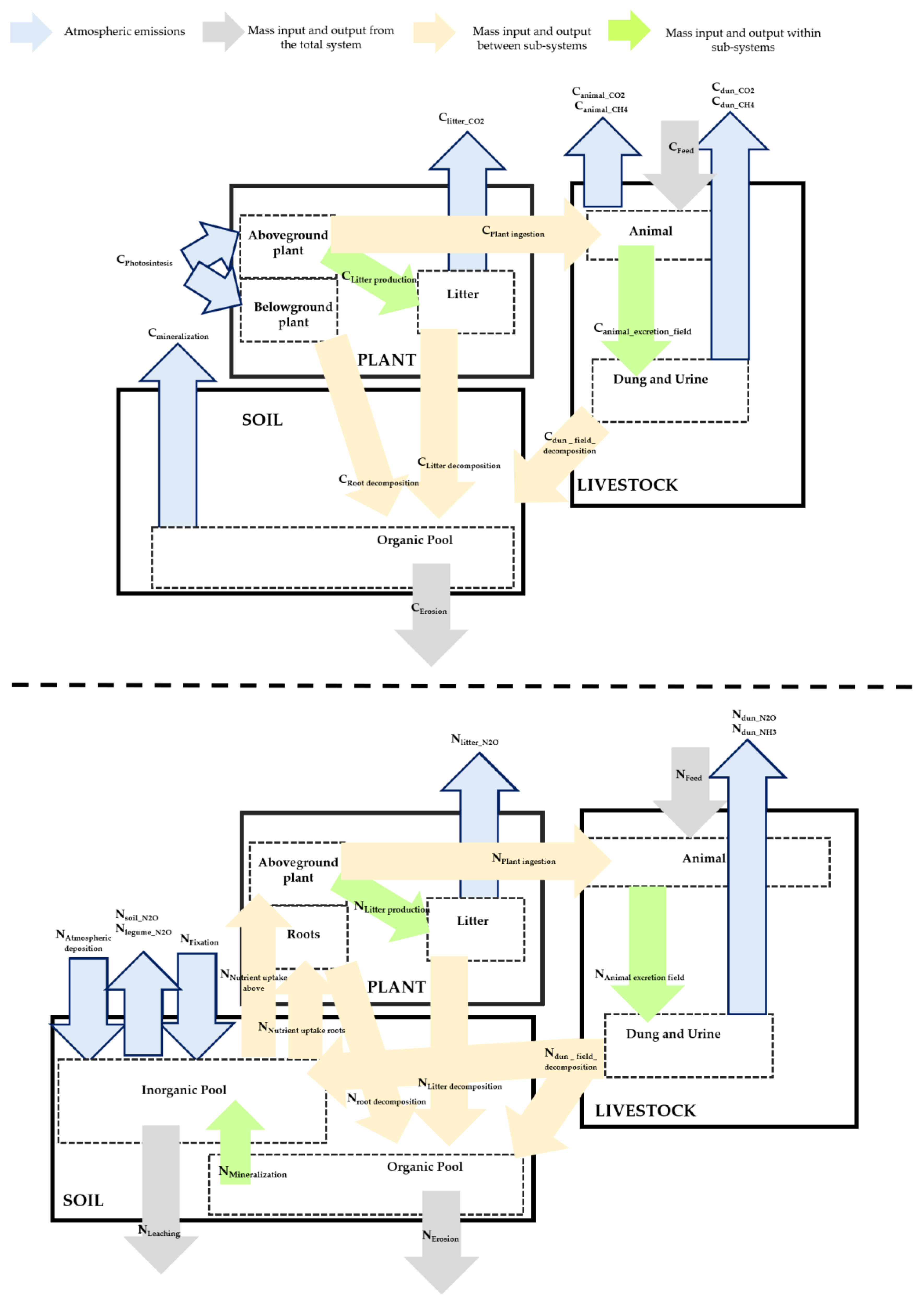
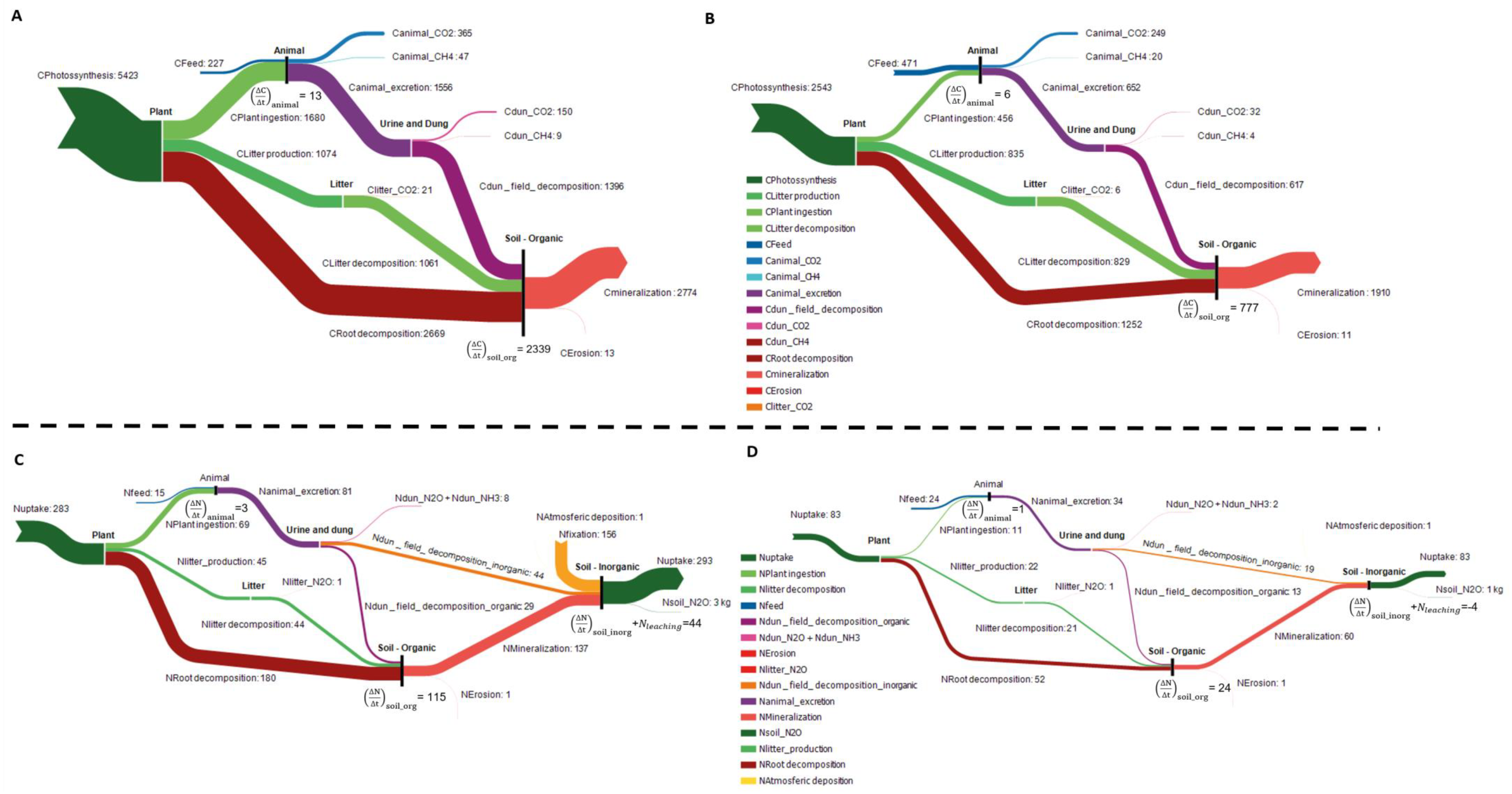
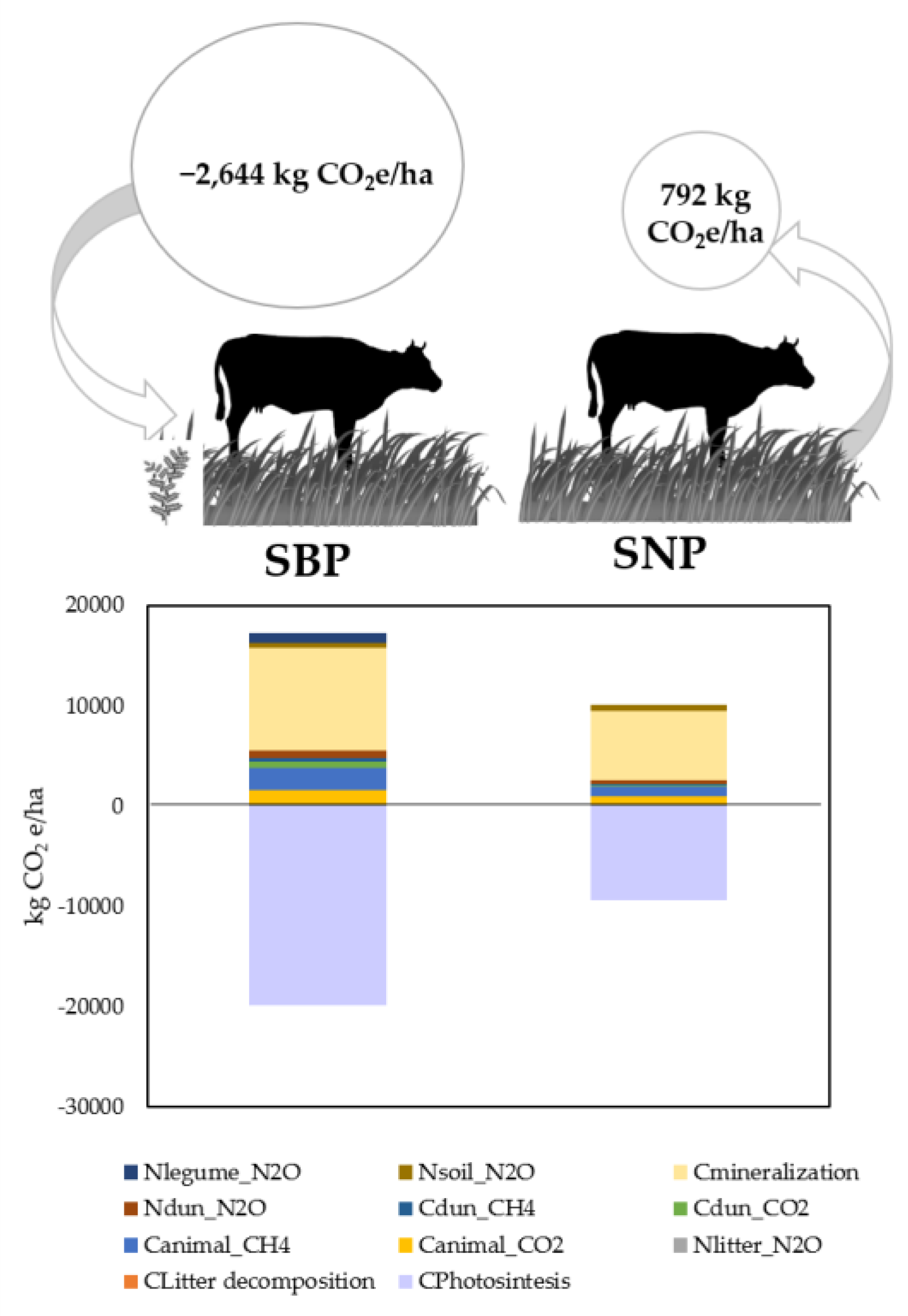
Table 1.
Averages of parameters measured in the study farms for sown biodiverse permanent pastures (SBP) and semi-natural pastures (SNP). Minima and maxima for all farms and years are also indicated. DM—Dry Matter; LU—Livestock Units; SOM—Soil Organic Matter.
Table 1.
Averages of parameters measured in the study farms for sown biodiverse permanent pastures (SBP) and semi-natural pastures (SNP). Minima and maxima for all farms and years are also indicated. DM—Dry Matter; LU—Livestock Units; SOM—Soil Organic Matter.
| Parameter | Description | Unit | SBP | SNP | ||
|---|---|---|---|---|---|---|
| Mean | Minimum-Maximum | Mean | Minimum-Maximum | |||
| Pabove | Aboveground productivity | kg DM/ha.yr | 6770 | 2110–10,680 | 3690 | 1501–7540 |
| Pstock | Stocking rate | LU/ha | 0.91 | 0.35–1.53 | 0.39 | 0.02–0.81 |
| SOM | Average SOM concentration | % | 2.17 | 0.45–5.60 | 1.77 | 0.55–4.70 |
| Annual SOM increment 1 | Percentage point per year | 0.30 | −2.07–2.70 | 0.11 | −0.70–1.30 | |
| Tair | Air temperature | °C | 18 | 17–21 | 18 | 17–21 |
1 Annual SOM increments were calculated as the difference between average SOM concentrations in two consecutive years.
Table 2.
Description of all variables used in this paper to depict flows. All variables are measured in kg (of carbon or nitrogen) per hectare and year.
Table 2.
Description of all variables used in this paper to depict flows. All variables are measured in kg (of carbon or nitrogen) per hectare and year.
| Designation in This Paper | Description |
|---|---|
| Carbon taken up by photosynthesis | |
| Carbon in roots decomposing in soil | |
| Carbon in the produced litter | |
| Carbon in litter decomposing in soil | |
| Carbon emitted as CO2 from litter deposition | |
| Carbon ingested by animals by eating plants | |
| Carbon uptake by animals through supplemental feed | |
| Carbon emitted as CO2 from animal respiration | |
| Carbon emitted as CO2 from animal enteric fermentation | |
| Carbon excreted by animals as urine and dung | |
| Carbon emitted as CO2 through aerobic mineralization of urine and dung from animal excretion | |
| Carbon emitted as CH4 through anaerobic mineralization of urine and dung from animal excretion | |
| Carbon from urine and dung deposited in the field that decomposes into the soil | |
| Carbon lost by soil erosion | |
| Carbon lost as CO2 from organic matter decomposition | |
| Nitrogen uptake by plants | |
| Nitrogen in roots decomposing in soil | |
| Nitrogen in the produced litter | |
| Nitrogen in litter decomposing in soil | |
| Nitrogen emitted as N2O after litter decomposition and nitrification | |
| Nitrogen ingested by animals by eating plants | |
| Nitrogen uptake by animals through supplemental feed | |
| Nitrogen excreted by animals through urine and dung | |
| Nitrogen from dung deposited in the field that decomposes into the soil organic pool | |
| Nitrogen from urine and dung deposited in the field that decomposes into the soil inorganic pool |
Table 3.
Carbon (C) and nitrogen (N) sub-system balance equations for BalSim. The variables indicated in black were estimated using a combination of measured data and parameters collected from the literature, and variables in blue are unknown in each equation. The variables are explained in Table 2.
| Sub-System | Balance | Balance Equation for C | Balance Equation for N |
|---|---|---|---|
| Plant | Plant and litter | ||
| Livestock | Animal | ||
| Dung and urine | |||
| Soil | Organic pool | ||
| Inorganic pool | - |
Table 4.
The full list of parameters taken from the literature and used in the mass balances of plants, animals and soil. DM—Dry matter; LU—Livestock unit; SBP—Sown biodiverse pastures; SNP—Semi-natural pastures.
Table 4.
The full list of parameters taken from the literature and used in the mass balances of plants, animals and soil. DM—Dry matter; LU—Livestock unit; SBP—Sown biodiverse pastures; SNP—Semi-natural pastures.
| Parameter | Description | Unit | SBP | SNP | Reference |
|---|---|---|---|---|---|
| Carbon content in the aboveground part of the plant | kg C/kg DM | 0.45 | 0.35 | [22] | |
| Nitrogen content in the aboveground part of the plant | kg N/kg DM | 0.02 | 0.01 | [22] | |
| Carbon content in the belowground part of the plant | kg C/kg DM | 0.45 | 0.35 | [22] | |
| Nitrogen content in the belowground part of the plant | kg N/kg DM | 0.03 | 0.01 | [22] | |
| C | Aboveground plant C:N ratio | kg C/kg N | 40 | 24 | Calculated (using Cabgplant/Nabgplant) |
| Aboveground plant C:N ratio | kg C/kg N | 15 | 25 | Calculated (using Cblgplant/Nblgplant) | |
| Root to shoot ratio | kg DM below/kg DM above | 0.98 | 0.98 | [21] | |
| Litter fraction calculation parameter | kg litter/kg DM | 0.39 | 0.62 | [21] | |
| Emission factor for N2O in litter | kg N-N2O/kg N litter | 0.0049 | 0.0049 | [23] | |
| Emission factor for CO2 in litter | kg C-CO2/kg C litter | 0.0049 | 0.0049 | Calculated (Section 2.3.1) | |
| Animal annual growth | kg LW/LU.yr | 289.9 | 289.9 | [24] | |
| Animal carbon content | kg C/kg DM | 0.487 | 0.487 | [25] | |
| Animal nitrogen content | kg N/kg DM | 0.114 | 0.114 | [25] | |
| Nitrogen cow excretion | kg N/head.yr | 105 | 105 | [23] | |
| Nitrogen calf excretion | kg N/head.yr | 44 | 44 | [23] | |
| Dung and urine C:N ratio | kg C/kg N | 19.1 | 19.1 | [26] | |
| Feed C:N ratio | kg C/kg N | 19.53 | 19.53 | [22] | |
| Emission factor for CH4 in calves | kg CH4/head.yr | 19.6 | 19.6 | [27] | |
| Emission factor for CH4 in cows | kg CH4/head.yr | 81.3 | 81.3 | [27] | |
| Emission factor for N2O in dung and urine | kg N-N2O/kg N excreted | 0.02 | 0.02 | [27] | |
| Emission factor for NH3 in dung and urine for calves | kg N-NH3/kg N dung | 0.06 | 0.06 | [23] | |
| Emission factor for NH3 in dung and urine for cows | kg N-NH3/kg N dun | 0.1 | 0.1 | [23] | |
| Emission factor for CH4 in dung and urine | kg CH4/LU.yr | 13 | 13 | [28] | |
| C | Soil C:N ratio | kg C/kg N | 19.695 | 31.955 | Calculated (Section 2.3.3) |
| Soil density | g/cm3 | 1.34 | 1.34 | [29] | |
| Nitrogen from legume plants | kg N fixed/kg DM | 0.026 | 0 | [27] | |
| Nitrogen deposited from the atmosphere | kg N/ha | 1.06 | 1.06 | [14] | |
| Soil lost by erosion | Mg soil/ha.yr | 1.030 | 1.030 | [30] | |
| Emission factor for N2O from legume plants | kg N-N2O/kg N fixed | 0.0125 | 0.0125 | [31] |
Table 5.
Non-CO2 outflows from the pasture system per hectare and kilogram of live weight of the animal. The flows are defined in Table 2. The variables are explained in Table 2. LU—Livestock unit; LW—Live weight.
| Flow | SBP | SNP | Unit |
|---|---|---|---|
| 411 | 172 | kg CO2e/ha.yr | |
| 2190 | 919 | kg CO2e/ha.yr | |
| + | 763 | 320 | kg CO2e/ha.yr |
| 258 | 73 | kg CO2e/ha.yr | |
| 577 | 577 | kg CO2e/ha.yr | |
| 931 | 0 | kg CO2e/ha.yr | |
| Total per hectare | 5131 | 2061 | kg CO2e/ha.yr |
| Total per LU | 5517 | 5285 | kg CO2e/LU.yr |
| Total per LW | 17.0 | 16.3 | kg CO2e/kg LW |
Table 6.
Results for the application of the model for the three scenarios. DM—Dry matter; GHG—Greenhouse gases; LU—Livestock unit; LW—Live weight; —Aboveground productivity; —Litter fraction; —Stoking rate; SOM—Soil Organic Matter.
Table 6.
Results for the application of the model for the three scenarios. DM—Dry matter; GHG—Greenhouse gases; LU—Livestock unit; LW—Live weight; —Aboveground productivity; —Litter fraction; —Stoking rate; SOM—Soil Organic Matter.
| Scenario S1 | Scenario S2 | Scenario S3 | |||||
|---|---|---|---|---|---|---|---|
| SBP | SNP | SBP | SNP | SBP | SNP | Unit | |
| 12,240 | 7380 | 7760 | 3690 | 3060 | 1845 | kg DM/ha.yr | |
| 1.86 | 0.78 | 1.50 | 0.68 | 0.79 | 0.39 | LU/ha | |
| Average SOM concentration | 5.60% | 4.70% | 2.17% | 1.77% | 2.17% | 1.77% | % |
| SOM increment | 0.55% | 0.08% | 0.60% | 0.20% | 0.30% | 0.10% | Percentage point per year |
| 0.39 | 0.65 | 0.39 | 0.82 | 0 | 0 | kg litter/kg DM | |
| Feed | 8.03 | 7.46 | 15.69 | 9.93 | 9.42 | 6.01 | kg feed DM/day |
| GHG balance | −4410 | 4544 | −6614 | 1195 | −3825 | 382 | kg CO2e/ha.yr |
| Non-CO2 emissions | 16.1 | 14.0 | 15.5 | 14.1 | 15.2 | 15.7 | kg CO2e/kg LW |
| Closure organic C model | 100 | 100 | 100 | 100 | 21 | (−) 7 | % |
| Closure inorganic N model | 91 | 89 | 89 | 100 | 47 | 75 | % |
Table 7.
Results for the application of the model for each year between 2001-2005 for the SBP. The flows are defined in Table 2. DM—Dry matter; GHG—Greenhouse gases; LU—Livestock unit; LW— Live weight; —Aboveground productivity; —Litter fraction; —Stoking rate; SBP—Sown biodiverse pastures; SOM—Soil Organic Matter.
| Parameter/variable | 2001–2002 | 2002–2003 | 2003–2004 | 2004–2005 | Unit | |
|---|---|---|---|---|---|---|
| Measured Data | 5985 | 8230 | 3966 | 3728 | kg DM/ha.yr | |
| 0.73 | 1.21 | 0.96 | 0.35 | LU/ha | ||
| 0.19 | 0.74 | 0.34 | 0.12 | Percentage point per year | ||
| Average SOM concentration | 1.50 | 1.51 | 2.26 | 2.06 | % | |
| Air temperature | 17.40 | 17.25 | 17.75 | 18.46 | °C | |
| GHG Balance | 323 | 536 | 423 | 156 | kg CO2e/ha.yr | |
| 1720 | 2856 | 2256 | 834 | kg CO2e/ha.yr | ||
| + | 599 | 995 | 785 | 290 | kg CO2e/ha.yr | |
| 330 | 365 | 15 | 250 | kg CO2e/ha.yr | ||
| 561 | 557 | 570 | 590 | kg CO2e/ha.yr | ||
| 911 | 1,253 | 604 | 567 | kg CO2e/ha.yr | ||
| Total per hectare | 4445 | 6562 | 4653 | 2688 | kg CO2e/ha.yr | |
| Total per LU | 6085 | 5411 | 4859 | 7593 | kg CO2e/LU.yr | |
| Total per LW | 18.80 | 16.72 | 15.01 | 23.46 | kg CO2e/kg LW | |
| Model Variables | 5840 | 5838 | 5836 | 5837 | kg C intake/day | |
| 0.25 | 0.25 | 0.25 | 0.25 | kg N intake/day | ||
| 0.51 | 0.41 | 0.035 | 0.62 | kg litter/kg DM | ||
| 0.19 | 1.09 | 1.95 | 0.85 | kg DM below/ kg DM above | ||
| 26.32 | 19.74 | 18.66 | 20.12 | Adimensional (−) | ||
| Balance closure | Organic C model | 100 | 100 | 100 | 100 | % |
| Inorganic N model | 72 | (−) 69 | (−) 75 | 90 | % |
© 2018 by the authors. Licensee MDPI, Basel, Switzerland. This article is an open access article distributed under the terms and conditions of the Creative Commons Attribution (CC BY) license (http://creativecommons.org/licenses/by/4.0/).
Share and Cite
MDPI and ACS Style
Teixeira, R.F.M.; Barão, L.; Morais, T.G.; Domingos, T. “BalSim”: A Carbon, Nitrogen and Greenhouse Gas Mass Balance Model for Pastures. Sustainability 2019, 11, 53. https://doi.org/10.3390/su11010053
AMA Style
Teixeira RFM, Barão L, Morais TG, Domingos T. “BalSim”: A Carbon, Nitrogen and Greenhouse Gas Mass Balance Model for Pastures. Sustainability. 2019; 11(1):53. https://doi.org/10.3390/su11010053
Chicago/Turabian StyleTeixeira, Ricardo F.M., Lúcia Barão, Tiago G. Morais, and Tiago Domingos. 2019. "“BalSim”: A Carbon, Nitrogen and Greenhouse Gas Mass Balance Model for Pastures" Sustainability 11, no. 1: 53. https://doi.org/10.3390/su11010053
Note that from the first issue of 2016, this journal uses article numbers instead of page numbers. See further details here.